Abstract— We describe a method using statistical hypothesis test for handling the unsuccessful results of partial exploration of the state space of marked graphs PN systems. The first contribution of our method is the estimation of the probability distribution function of the state space of PN systems. The second one is to give completeness to the unsuccessful results by determining reachability with a level of confidence through the test. In this paper we focus in PN systems with the form of structurally bounded marked graphs with probability distribution of their set of reachable markings believed to be normal.
Index Terms—Petri nets, Hypothesis test, Reachability Problems, State space
I. INTRODUCTION
UR work focuses on determining the existence of undesired states without having to explore the entire state space generated from large and bounded Petri net (PN) systems. With a heuristically guided partial exploration of the state space we visit and register a number of states believed to be smaller than the complete state space and search for the target state.
Works related to determining reachability in the state space generated from PN systems usually utilize reachability graphs exploring the entire state space but limited due to the state space explosion problem [1]. On the other hand, the list of works exploring only a portion of the state space is large but many of them face convex termination, lack of conclusiveness and their efficiency is ignored [1-4], although good results exist in the confines of specific practicability.
Lack of conclusiveness represents a wasted cost, therefore upon unsuccessful search, we will treat the results with a statistical hypothesis tests to decide with a level of confidence if the undesired state exists or not. This novel approach integrates certainty to the incompleteness of the heuristically guided partial exploration of the state space using a test for proportions.
First, from the unsuccessful results of the partial exploration, we will utilize the explored states as a sample for statistical inference. We will estimate the probability distribution function (PDF) of the state space, the proportion of states with the same cardinality as the undesired state and
Manuscript received March 5, 2011.
Eleazar Jimenez Serrano is with the Department of Automotive Sciences, Graduate School of Integrated Frontier Sciences, Kyushu University, Fukuoka city, Japan 819-0395 (phone/fax: 092-802-6903; e-mail: eleazar.jimenez.serrano@kyudai.jp).
define a hypothesis test to determine if the undesired state exists or not in the state space. We believe we can accurately estimate the proportion of states in the state space with same cardinality as the undesired state and obtain a reliable result with the hypothesis test. With this, our partial exploration can have either a conclusive outcome if the undesired state was found or provide a level of confidence indicating if such state is likely to exist in the state space.
Second, in this paper we will analyze how appropriate is treating the results of the partial exploration of the state space with a hypothesis test for proportions in PN systems with the structure of bounded marked graphs. For this, two small examples will demonstrate that for this subclass of PN the test can give correct results.
This paper is self-contained and arranged in the following order: section two contains a small theoretical background about hypothesis test and PN systems. Section three presents the fundaments of our method regarding the probability distribution of the state space of a PN system (a distribution which belongs to the state space of the PN without tokens), the reachability analysis with partial exploration and the form of our hypothesis test. Section four describes the algorithm for partial exploration of the state space and three sorting routines for making it heuristically guided. Section five describes the estimated normal probability distribution function of the state space. Section six contains the two theoretical examples and at the end are some conclusions.
II. HYPOTHESIS TEST AND PNSYSTEMS
A statistical hypothesis test uses observed data from an experiment for making decisions about the acceptance or not of specific characteristics in the entire population. In our research we will use them to provide a level of certainty and closure to the unsuccessful search of the partial exploration in reachability problems of PN systems for determining the existence or not of undesired states.
Assuming the size of the state space of the PN system is large and unknown, we have to calculate the number n of states we need to explore (the number of samples). The number of states we need to explore has to be enough in order not to compromise the veracity of the hypothesis test.
Then, we transform the reachability problem of the undesired state in terms of deciding with a hypothesis test for proportions if there is enough evidence indicating that the state being searched exists or not in the state space.
Let us start our treatment with a brief introduction of the PN theory. For reference and proofs on boundedness in PN systems and the theorems in the section three we address the reader to [3, 5-6].
Hypothesis Test for Unsuccessful Partial
Explorations of State Spaces of Petri Nets
Eleazar JIMENEZ SERRANO, Member, IAENG
A. Petri Nets
A Petri net is a tuple N = (P, T, I, O, Q), where P is a finite non-empty set of i places, T is a finite non-empty set of j transitions, I is the set of directed arcs connecting places to transitions, O the set of directed arcs connecting transitions to places and Q is a capacity function for the places mapping P Z+. Places are graphically represented by circles, transitions by rectangles and all directed arcs by arrows. The pre-conditions of a transition t are in the set of input places •t
and the post-conditions in t•. The pre-events of a place p are in the set •p and the post-events in the set p•.
A PN is called pure when there are no self-loops. A state machine is a PN such that |•t|=|t•|=1. A marked graph is a PN such that |•p|=|p•|=1.
The way to represent a state of the system is by putting tokens in the corresponding places. Tokens are black dots that exist only in the places. The function m called marking maps P Z+, and m0 is the initial marking. A PN with initial
marking is called a PN system and will be denoted by (N, m0).
We say that a place p is marked when m(p) > 0. The finite set of all possible markings (i.e. the reachability space) of (N, m0)
is denoted by R. The sum of all tokens in a marking m is defined with the function card(m).
The number of states that a PN system can generate depends on the input and output arcs, the initial marking and the way how the occurrence of transitions is specified. Occurrence of single transition is carried out for the generation of the complete state space of a PN system and mainly used for analysis purposes. Occurrence of concurrent transitions is implemented for generating possibly not-complete state spaces and it is assumed in the rest of this paper except if specified differently.
The sets of arcs I and O can be represented with the pre-incident matrix and the post-incident matrix I and O respectively having both i rows and j columns, with values of [I(pi, tj)] and [O(pi, tj)] respectively, and a marking m as a
vector m Zi defining the state of the system.
The token game refers to the way how the dynamic behavior of the system is described with the markings evolution (the removal of existing tokens and the creation of new tokens), according with the firing of enable transitions. The enabling rule is defined as: a transition t* T is said to be enabled at a given marking m if every of its input places has at least as many tokens as the weight of the arcs joining it and every of its output places has a number of tokens smaller than the sum of their current marking plus the weight of the arc connecting them. The set of all enabled transitions at a marking m is denoted with T(m)*.
A transition is called fireable if it is enabled. A fireable transition may fire, eliminating the marking m and creating the new marking m‟.
Using the initial marking vector m0, the next marking
vector m is mathematically calculated with the state transition function m = m0+(O−I)×σ. In this formula,
σ is a firing count vector representing the number of times
every transition has fired.
The maximal number γ of tokens that could exist in any PN system (N, m0), with qα as the finite tokens capacity of the αth
place, is given by
i
q
1)
1
(
. (1)
A PN system (N, m0) is bounded if all places have finite
tokens capacity; it is bounded at a number ≤γ of tokens in every marking of its state space.
III. REACHABILITY IN PNSYSTEMS
State spaces are derived from a model of system behavior, like PN systems. Verification of specific properties of the complete state space is in general necessary to guarantee the correct functionality of the system and verify the compliance of design specifications. Unfortunately the usage of verification techniques of the state space is limited due to its possibly exponential growth of size, especially when concurrent occurrences of events exist in the system.
A PN N‟ (without tokens) with all places having finite tokens capacity has a number of markings given by
i
q
11
. (2)
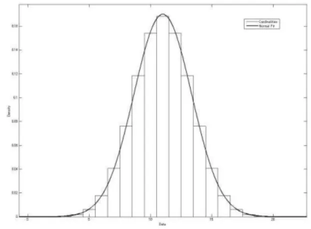
Let us denote U as the set of all markings that could exist in a PN N‟ without tokens, with size of Ω. For every mU let us define the variable X (number of tokens in m) as follows:
)
(
)
(
m
card
m
X
. (3)Independently of the number of places and tokens capacity in N‟, if mU we create a histogram of X(m), we get a distribution of frequencies of X as seen in the fig.1, with the appearance of a normal probability distribution function, i.e.
X~N(μ, 2) where μ= /2.
A. Complete Exploration
In a PN system (N‟, m0) and its set of reachable markings R,
for every mR the following two theorems belong by now to folk knowledge.
Theorem 1. A PN system (N‟, m0) with m0 U generates a
state space R with markings belonging to U. □
Theorem 2. A PN system (N‟, m0) generates zero markings
when the initial marking has no tokens, i.e. card(m0)=0, or
when card(m0)=γ. □
Let us define the variable Y as follows for a PN system (N‟,
m0) and every mR
).
(
)
(
m
card
m
Y
(4)We can create a histogram of Y(m) and identify the distribution of frequencies of Y if we explore the complete set of reachable markings R.
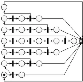
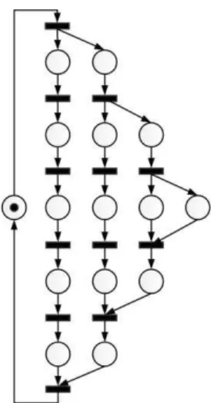
Let us assume the PN system (N„, m0) is the marked graph
from the fig.2. After complete exploration of its set R, the distribution of frequencies of Y is seen in the fig.3, with the appearance of a normal probability distribution function, i.e.
Y~N(
x
, s2).The probability distribution function turns out to be normal for the PN system in the fig.2 and the parameter easily calculated because the number ω of states in R is small, but in very large PN systems where the complete exploration of the reachability space is not feasible, this information is not available to the analyst.
B. Partial Exploration
For the reachability problem of finding a target marking mt
R with cardinality of c without exploring the complete set R, we can conduct a partial exploration with a heuristic algorithm targeting to visit markings with cardinality of c and
to stop the search upon finding the target marking or visiting ω pY(mt) markings with cardinality c, i.e. the number of
states in R multiplied by the probability of the marking mt
with cardinality c [7-8]. The disadvantage of this approach is that knowledge of the PDF is ignored. Since we ignore the number of states we should stop the exploration, complete exploration of the reachability space R is possible to happen. For the case when we ignore the information about the set R, we can use the information from the set U. We ignore how the markings in R are distributed in U, but since we know R U, the maximal number of markings with cardinality of c that could exist in R is Ω pX(mt).
For the reachability problem of finding a target marking mt
R with cardinality of c without exploring the complete set R, we can conduct a partial exploration with a heuristic algorithm targeting to visit markings with cardinality of c and to stop the search upon finding the target marking or visiting Ω pX(mt) markings with cardinality c. The disadvantage of
this alternative approach is that a full exploration of the complete reachability space R is also possible to happen.
C. Probabilistic Termination
The two approaches described before seem correct in theory, but with ignored efficiency and possible convex termination, leading to a possible complete exploration. Targeting to visit specified markings is not a guarantee of reaching those markings; therefore a sample size is calculated for termination and completeness.
The heuristic algorithms could also stop the search after visiting a number of markings determined by the formula in (5) to calculate the number of samples n in a large population for a proportion [9-10]
2 2
/
))
(
1
)(
(
m
p
m
e
p
Z
n
t
t . (5)The value of n is adequate whenever we know size ω of the set of reachable markings R and the proportion pY(mt). For the
case when we ignore those values and use pX(mt), the number
n is just as reference to determine an approximate value.
D. Standard Hypothesis Test
The results of the unsuccessful search of the target marking
mt with partial exploration can be treated with a hypothesis
test to provide certainty and completeness.
We define the pseudo-random variable Q as follows for each marking m registered in the exploration
c
m
card
if
c
m
card
if
m
Q
)
(
0
)
(
1
)
(
. (6)From the probability mass function (PMF) pQ(mt), we
obtain q as the proportion of markings with the same cardinality as mt and state the following test:
Y Y
p
q
H
p
q
H
:
:
1 0
Fig. 2. Structurally bounded marked graph PN system.
The test statistic computed for the hypothesis test of proportions is
n
p
p
p
q
/
)
ˆ
1
(
ˆ
ˆ
. (7)We will use a 95% level of significance in our hypothesis test. The standard normal z-table gives a value of 1.645.
The decision obtained with this hypothesis test will be: if we accept H0 as true it means there might not be other
markings with the same cardinality as the target marking, then the target marking is not in the set of reachable markings R of the PN system. On the other hand, if we cannot reject H1 then
it is probable that the target marking mt exists.
The appropriateness of the hypothesis test relies on the sampling method, the states registered (samples) and the proportion of markings pY in the set of reachable markings
with the same cardinality as the target marking. For this, in the next section we describe the former heuristic sampling method and describe two alternative methods. Later in the section five we will present how to utilize the samples for constructing the probability distribution function of R, how to estimate pY and will describe the statistical hypothesis test.
IV. HEURISTIC ALGORITHM OF PARTIAL EXPLORATION
The breadth-first based heuristic algorithm originally presented for the partial exploration of the state space for reaching a target marking mt is described as follows:
1: REG = m0 put m0 in register of markings
2: VIS = REG set of visited markings 3: repeat
4: mc = Top(VIS) get current marking
5: T(mc)* set of sorted enabled transitions at mc
6: if T(mc)* = then
VIS = VIS – mc and goto 12
7: = Top(T(mc)*)
8: mn = mc + (O – I) get next marking
9: if mn = mt then goto 13
10: if mn REG then
REG = REG + mn and VIS = VIS + mn
11: T(mc)* = T(mc)* –
12: until VIS = 13: end.
For the previous algorithm to be heuristically guided towards the target marking, the set T(mc)* is sorted with the
routine discussed next.
A. Rectilinear Distance Sorting
The sorting routine to obtain the set T(mc)* is described as,
for every firing vector T(mc)* enabling a transition t and
creating one next marking mn, the rectilinear distance RD()
is the sum of absolute values of the difference mn(p) – mt(p)
p P. A firing vector with zero rectilinear distance will be put at the top of the stack.
1: T1 = T(mc)*
2: repeat
3: read from T1
4: RD() = Sum(Abs(mn(p) – mt(p))) p P
5: put RD() in ET 6: delete from T1 7: until T1 =
8: T(mc)* = sorted T(mc)* by ET1 in ascending order
Although with a rectilinear distance sorting routine we still obtain a convex exploration, successfully cases are registered with analogous methods in [11-13].
On the other hand, in this paper we present two additional methods taking in consideration past and future marking results. Upon accomplishing to fill the tokens quota in places of the target marking, those partial findings are discarded with the rectilinear distance sorting routine because the metric is a total scalar measurement. Our proposals consider a more specific metric based on individual scalar measurements of tokens in each place for the reached markings.
B. Forward Sorting
One proposed routine to obtain the set T(mc)* is described
as, for every firing vector T(mc)* enabling a transition t
and creating one next marking mn, if p t• such that mn(p) =
mt(p), then the corresponding firing vector will be put at the
top of the stack. The firing vector enabling transitions all together having the largest number of pos-places fulfilling the condition will be at the top of the stack.
1: T2 = T(mc)*
2: repeat
3: read from T2
4: FW() = {p t• | t is enabled at and mn(p) = mt(p)}
5: s() = card(FW()) 6: put s() in ET2 7: delete from T2 8: until T2 =
9: T(mc)* = sorted T(mc)* by ET2 in descending order
In order to fulfill the tokens quota in the places, the previous algorithm was specifically designed to foreseeing the marking in the places.
C. Backward Sorting
In our second proposal, for every firing vector T(mc)*
enabling a transition t and creating one next marking mn, if p
•t such that mc(p) = mt(p), then such firing vector will not be
put at the top of the stack. The firing vector enabling transitions all together having the largest number of pre-places fulfilling the previous condition will be at the bottom of the stack.
1: T3 = T(mc)*
2: repeat
3: read from T3
4: BW() = {p •t | t is enabled at and mc(p) = mt(p)}
8: until T3 =
9: T(mc)* = sorted T(mc)* by ET3 in ascending order
Upon fulfilling the tokens quota in some places, the previous algorithm was designed to avoid those places to lose their token quota immediately. And a more sophisticated algorithm could include a second sorting using the index ET2 from the previous algorithm.
V. ASSUMED PDF OF THE SET OF REACHABLE MARKINGS
Progressions of the markings in a PN system are dependent of the previous marking and the inherent non-determinism in the network. Statistical methods use random samples of independent observations all having the same probability of being selected. Since we ignore the set of reachable markings R, it is impossible to conduct a proper random sampling and any exploration-based samplings seems inadequate in principle.
Probability samples can only be used to create mathematically sound statistical inferences about a larger target population. Non-probability sampling has no way of measuring their bias or sampling error.
Works in [14-20] discuss the estimation of state space parameters using different sampling techniques, but none of them alert about this inadequacy. Although any state space exploration algorithm, saying depth-first, breath-first, random walks, etc., might seem inadequate because they are dependent on the system‟s progression, in fact the algorithms provide a systematic sampling, a type of probability sampling, however no details on the sampling procedure are given.
Our exploration algorithms and the three sorting routines give non-probability samplings and their samples will be biased towards the target marking. The empirical probability mass function (PMF) constructed with the results of the sampling will be fitted to a normal PDF since it is believed the state space has such distribution.
The results in [8] fitted the empirical PMF to a normal distribution with mean
x
ˆ
equal to the cardinality of the target marking and standard deviations
ˆ
equal to the absolute value of resting the cardinality of the initial marking to the cardinality of the target marking. The empirical PMF fitted to a normal PDF can be seen in the fig.4. Although good results were obtained for some PN systems, the method lacks of generalization.In this paper we focus on bounded marked graph PN systems which could produce normality in the set R, like the PN system in the Fig.2. They have mean
x
ˆ
and variances
ˆ
2calculated from the sampled markings. The mean is near the cardinality of the target marking and the maximal sampling error for the mean equal to |
x
–x
ˆ
|.Our proposed fitted normal PDF for the set R is defined as
x ss x
Y
x
s
Y
x
s
f
y
P
ˆ
3
ˆ
ˆ
3
ˆ
)
(
]
ˆ
3
ˆ
ˆ
3
ˆ
[
. (8)The function f(x) corresponds to the normal distribution and the 3
s
ˆ
assumption is adopted from the “68-95-99.7” statistical rule of the normal distribution.A. Hypothesis Test with the Fitted Normal PDF
The form of the hypothesis test presented in the section 3-D does not change. The only difference is that the proportion of markings pY used in the test corresponds to the probability
PY[Y=card(mt)], i.e. the probability of the cardinality of the
target marking with the fitted normal PDF of the set R. VI. THEORETICAL EXAMPLE
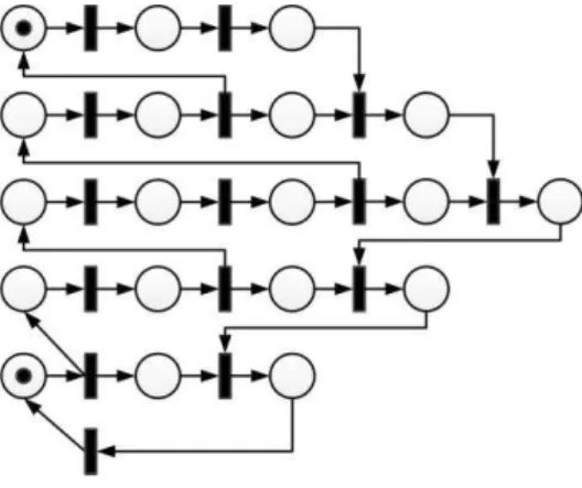
Let us utilize the PN systems in the figure 5 and 6. In this paper the PN systems under study are restricted to be a bounded marked graph. The nets are believed to have normality in their set of reachable markings R, similar to the one of the PN system in the fig.2.
The PN systems are rather small but the usability of the hypothesis test in larger nets is straightforward.
We conducted partial exploration of different markings using the three sorting routines: rectilinear distance (RD), forward distance (FD) and backward distance (BD). Sample size was fixed at 20 based on all sample size results. All explorations were unsuccessful, but only one sample was used in the hypothesis test.
To determine the appropriateness of the test for these examples, by first comparing the mean and variance of the set of reachable markings R with the ones from the sample (Table I) we observe a significant difference exists only in one parameter.
Our second comparison is on the value of the proportion of markings with same cardinality as the target marking of the set
Fig. 4. Empirical PDF of the set R.
of reachable markings R and the ones from the sample (Table II). Two target markings were selected in each example for evaluation. A correct correlation is observable and a significant difference exists in only one result.
Finally, from the results in the hypothesis test, Table III shows the value of the test statistic, the decision with the test and the evaluation of the decision based on the actual existence of the target marking in the complete state space. Just one decision was taken incorrectly.
VII. CONCLUSION
Using a hypothesis test on the unsucceeded results of the heuristically guided partial exploration seems appropriate to determine if a target marking exists or not in the probably normal state space of a structurally bounded marked graph PN system. Comparison of the estimated values presents good result and the evaluation of the decision shows only one incorrect decision. We conclude this kind of test might be appropriate to use on larger PN systems just upon further research.
Although it is not guaranteed yet that the target marking would be found with our heuristically guided partial exploration algorithm without complete exploration of the set of reachable markings R, the idea of using a complementary hypothesis test to analyze reachability problems have certain level of effectiveness in this specific subclass of PN systems. Criterions about determining normality based on the PN model are in the next steps.
REFERENCES
[1] G. Holzmann, “Algorithms for Automated Protocol Verification,”
AT&T Technical Journal (69)2, pp.32-44, 1988.
[2] Matthias Kuntz and Kai Lampka, Probabilistic Methods in State
Space Analysis. Validation of Stochastic Systems, LNCS 2925,
Springer, Heidelberg, 2004, pp. 251-266.
[3] Kurt Jensen and Lars M. Kristensen, Coloured Petri nets. Modeling
and Validation of Concurrent Systems, Springer-Verlag Berlin
Heidelberg, 2009.
[4] Gianfranco Ciardo, “Reachability Set Generation for Petri Nets: Can Brute Force Be Smart?,” in Proc. 25th Int. Conf. on Applications and Theory of Petri Nets, LNCS 3099, 2004, pp.17-34.
[5] T. Murata, “Petri nets: Properties, Analysis and Applications,” in Proc.
IEEE, vol.77, 1989, pp.541-580.
[6] Andrei Karatkevich, Dynamic Analysis of Petri Nets-Based Discrete
Systems, Springer-Verlag Berlin Heidelberg, 2007.
[7] Eleazar Jiménez Serrano, “A Probability-based State Space Analysis of Petri Nets,” Inst. of Electronics, Information and Communication
Engineers (IEICE), Technical Report vol.110, no.283, 2010, pp.7-12.
[8] Eleazar Jiménez Serrano, “Using Metaheuristics and SPC in the Analysis of State Spaces of Petri Nets,” Medwell Journal of Engineering and Applied Sciences, vol.5, no.6, 2010, pp.413-419.
[9] Eleazar Jiménez Serrano, “Improved Estimation of the Size of the State Space of Petri Nets for the Analyis of Reachability Problems,” in Proc.
of the 5th WSEAS European Computing Conference 2011, to be
published.
[10] W. G. Cochran, Sampling Techniques, 2nd Edition, John Wiley and Sons, Inc. 1963.
[11] K. E. Torku and B. M. Huey, “Petri Nets Based Search Directing Heuristic for Test Generation”, in IEEE Proc. of 20th Conf. on Design Automation, 1983, pp.323-330.
[12] K. M. Passino and P. J. Antsaklis, “Artificial Intelligence Planning Problems in a Petri Net Framework,” in Proc. American Control
Conference, 1988, pp.626-631.
[13] K. M. Passino and P. J. Antsaklis, “Planning via Heuristic Search in a Petri Net Framework,” in Proc. of the IEEE Int. Symposium on
Intelligent Control, 1988, pp.350-355.
[14] James F. Watson III and Alan A. Desrochers, Methods for Estimating State-Space Size of Petri Nets, in Proc. of the IEEE International
Conference on Robotics and Automation, 1992, pp. 1031-1036.
[15] James F. Watson III and Alan A. Desrochers, State-Space Size Estimation of Conservative Petri Nets, in Proc. of the IEEE
International Conference on Robotics and Automation, 1992, pp.
1037-1042.
[16] James F. Watson III and Alan A. Desrochers, State-Space Size Estimation of Petri Nets: A Bottom-Up Perspective, IEEE
Transactions on Robotics and Automation, vol.10, no.4, pp. 555-561,
1994.
[17] Radek Pelánek and Pavel Simecek, “Estimating State Space Parameters,” Technical report FIMU-RS-2008-01.
[18] Radek Pelánek, “Properties of state spaces and their applications,” Int.
Journal on Software Tools Technology Transfer, pp.443–454,
Springer, Heidelberg, 2008.
[19] Radek Pelánek, “Fighting State Space Explosion: Review and Evaluation,” in Proc. of Formal Methods for Industrial Critical
Systems 2008, LNCS 5596, 2009, pp.37-52.
[20] Nicholas J. Dingle and William J. Knottenbelt, “State-Space Size Estimation By Least-Squares Fitting,” in Proc. 24th UK Performance
Engineering Workshop, 2008, pp.347–357.
TABLEI COMPARISON OF PARAMETERS
Example 1 Mean Var
True Value 3.05357 0.524351 Estimation 3.05000 0.786842
Example 2 Mean Var
True Value 4.00000 1.609760 Estimation 3.50000 0.789474 Fig. 6. Example 2 - Marked graph PN system.
TABLEII
COMPARISON OF PROPORTIONS –EXAMPLES 1&2
card(mt) ˆpY(mt) pY(mt)
2 0.21135 0.19117 3 0.44903 0.54943 2 0.10799 0.09077 3 0.38325 0.23048
TABLEIII EVALUATION OF DECISIONS
card(mt) TEST
STATISTIC DECISION EVAL