Can 3D Point Clouds Replace GCPs?

CAN 3D POINT CLOUDS REPLACE GCPs?

G. Stavropoulou, G. Tzovla, A. Georgopoulos

Laboratory of Photogrammetry, School of Rural & Surveying Eng. National Technical University of Athens, Iroon Potytechniou 9, 15780, Zografos, Athens, Greece

ginanoelma@yahoo.gr, georgiatzovla@gmail.com, drag@central.ntua.gr

KEY WORDS: Orthophotography, Close-range Photogrammetry, 3D point clouds, Single image resection, Cultural Heritage

ABSTRACT:

Over the past decade, large-scale photogrammetric products have been extensively used for the geometric documentation of cultural heritage monuments, as they combine metric information with the qualities of an image document. Additionally, the rising technology of terrestrial laser scanning has enabled the easier and faster production of accurate digital surface models (DSM), which have in turn contributed to the documentation of heavily textured monuments. However, due to the required accuracy of control points, the photogrammetric methods are always applied in combination with surveying measurements and hence are dependent on them. Along this line of thought, this paper explores the possibility of limiting the surveying measurements and the field work necessary for the production of large-scale photogrammetric products and proposes an alternative method on the basis of which the necessary control points instead of being measured with surveying procedures are chosen from a dense and accurate point cloud. Using this point cloud also as a surface model, the only field work necessary is the scanning of the object and image acquisition, which need not be subject to strict planning. To evaluate the proposed method an algorithm and the complementary interface were produced that allow the parallel manipulation of 3D point clouds and images and through which single image procedures take place. The paper concludes by presenting the results of a case study in the ancient temple of Hephaestus in Athens and by providing a set of guidelines for implementing effectively the method.

1. INTRODUCTION

1.1 Photogrammetry & Documentation of Monuments

Since the early years of the 20th century, photogrammetry has slowly but steadily gained ground over the traditional methods of cartography, not always without criticism. In the past, surveyors and cartographers often opposed to photogrammetric methods, raising questions over their quality and reliability. Additionally, the costs for precise metric cameras and the time-consuming analogue processes were undermining the merits of photogrammetry, leaving its methods largely unrecognized. In the more recent decades technological advances have enabled quicker and cheaper data acquisition and the simultaneous development of digital photogrammetry has facilitated the automation of many processes with applications in a wide variety of scientific fields. The constant improvements in both aerial and close range photogrammetry have allayed all negative discussion and now more that ever photogrammetric techniques are considered as an integral part of any survey.

In the field of Heritage preservation, many techniques have been implemented throughout the years, so as to achieve precise descriptive but, more importantly, accurate documentation of cultural sites. As defined by UNESCO in 1972, the geometric documentation of a monument may be described as “the action of acquiring, processing, presenting and recording the necessary data for the determination of the position and the actual existing form, shape and size of a monument in the three dimensional space at a particular given moment in time”. Complying with this definition, digital photogrammetry is widely used for measuring and obtaining the current condition of monuments, but also for monitoring decay and deformation and for producing metric outputs used as base for conservation and restoration plans. Rectified images and orthoimages are well-suited products

for such purposes as they combine metric characteristics with a high level of radiometric detail under relatively low production costs.

1.2 Terrestrial Laser Scanning for the documentation of monuments

Today two methods are usually applied for the documentation of cultural heritage (Dulgerler et al., 2007):  Simple topometric methods for partially or totally

uncontrolled surveys

 Surveying and photogrammetric methods for completely controlled surveys

In addition to those methods, 3D laser scanning has quickly become one of the most commonly used techniques for heritage documentation. The volume of points and high sampling frequency of laser scanning offers a great density of information, providing optimal surface models for applications of archaeological and architectural recordings. According to Boehler et al (2005) laser scanning can replace or complement methods used so far in metric cultural heritage documentation when complicated objects have to be recorded economically with moderate accuracy requirements. Indeed, the combination of laser scanning and close-range photogrammetry has often been implemented in the documentation of monuments (Bartos et al., 2011; Valanis et al, 2009; Kaehler & Koch, 2009; Mitka & Rzonca, 2009; Yastikli, 2007; Griesbach et al., 2004), as it eliminates the need of strict guidelines for image acquisition and time-consuming procedures for DSM generation.

time-consuming process, recently attempts have been made to take advantage of the primary form of 3D point clouds. This approach of using directly 3D points instead of a mesh was followed in a case study by Georgopoulos and Natsis (2008) and also constitutes an attempt of work presented in this paper.

1.3 Proposed Method

Despite the fact that the integration of data from both digital cameras and terrestrial laser scanners can result in very useful outputs, both methods have limitations that do not comply with the accuracy requirements of heritage recording. The poor edge definition of laser scanning and the need to determine the exterior orientation of the images demand complementary geodetic measurement of control points. Classical survey measurements provide accurate determination of specific points, which form a rigid framework within which the monument details from the photogrammetric survey are being placed. This framework provides strong interrelations of the measured points in 3D space, necessary as a base for the photogrammetric procedures (Georgopoulos & Ioannidis, 2004). Therefore, a large part of the data collection is dependent on surveying methods. Due to this dependency, photogrammetric methods are still largely regarded as an extension rather than an alternative of surveying measurements.

This subsequently leads to increased fieldwork and complicated procedures of data collection. Dallas refers in 1996 that one of the limitations of photogrammetric products is the complexity of the technique, which requires the input of specialists. Although the usage of laser scanners reduces the need for strict specification during image collection, the complexity remains in the surveying part of the procedure, which is by definition time-consuming.

In the current paper we explore the possibility of delivering high-quality photogrammetric products without the need of additional surveying procedures. Driven by the hypothesis that a dense and accurate point cloud can offer an abundant number of control points despite the poorly defined edges, an alternative method is proposed that is exempted from traditional surveying measurements. However, it should be mentioned that the proposed method does not refer to cases where an already coloured point cloud is available, i.e. a point cloud acquired from a laser scanner with an embedded or an attached digital camera. To assess the effectiveness of the method a case study in the temple of Hephaestus in Ancient Agora in Athens is presented.

2. METHODOLOGY

2.1 Algorithm development

For the assessment of the proposed method, an algorithm that allows the parallel manipulation of point clouds and images was developed in Matlab environment. Additionally a complementary interface (Fig. 1) was developed to facilitate the loading of the necessary data and the processes of point selection from both the images and the point cloud.

The user can choose between two different functions, orthophoto generation or implementation of 2D projective transformation, i.e. rectification. The necessary input data are a 3D point cloud in comma delimited ASCII form, a high-resolution image of the object that has not been subjected to any alterations or rotations, and the intrinsic parameters of

the camera in the case of orthophoto. The prior georeference of the point cloud is not necessary as the algorithm can operate with the reference system of the laser scanner point cloud. Complementary options allow the user to define the scale of the output and to insert an approximate distance from the object while acquiring the images. The interface supports the selection of control points from the point cloud and the image. However, the procedure can take place in different software and then the coordinates can be inserted as ASCII files in the software.

Figure 1: Interface for the developed algorithm

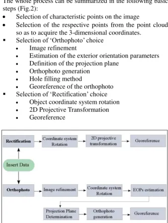
The whole process can be summarized in the following basic steps (Fig.2):

 Selection of characteristic points on the image

 Selection of the respective points from the point cloud so as to acquire the 3-dimensional coordinates.

 Selection of ‘Orthophoto’ choice  Image refinement

 Estimation of the exterior orientation parameters  Definition of the projection plane

 Orthophoto generation  Hole filling method

 Georeference of the orthophoto  Selection of ‘Rectification’ choice

 Object coordinate system rotation  2D Projective Transformation  Georeference

Figure 2: Diagram describing the basic steps of the algorithm

2.2 Orthophotography

projective transformation, Smith and Park (2000) with the absolute and exterior orientation using linear features and Wang (1992) with a rigorous photogrammetric adjustment algorithm based on co-angularity condition. However, space resection is the most commonly used technique to determine exterior orientation parameters.

Due to the non-linear nature of the collinearity equations the approximate values of the unknowns must first be determined. Taylor’s theorem is used to linearize the equations and an iterative least squares estimation process takes place to evaluate the six exterior orientation parameters Xo, Yo, Zo, ω, φ, κ. However, two things have to be considered at this stage.

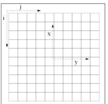
Firstly, the image coordinates that are used in the collinearity equations need to be refined and corrected for lens distortion. (Cooper & Robson, 1996; Kraus, 2003). Affine transformation is used to establish the relationship between the image coordinate system (i, j) and the photographic system (x, y) (Fig.3) and the interior orientation of the camera calibration is used to calculate the six parameters of the transformation (Κarras, 1998). The image coordinates transformation follows the correction for radial distortion. The user has the opportunity to run the algorithm even if he doesn’t have the parameters of the affine transformation of the lens distortion, although significant effects would appear in the accuracy of the final result. (Karras et al., 1998)

.

Figure 3: Image coordinate systems i, j and x,y

Secondly, the calculation of the approximate values of the unknowns is of crucial importance. The initial estimates must be close to the true values or else the system may not converge quickly or correctly (Ji, 2000). In aerial photogrammetry, the estimation of the initial values is an easy task but this is not the case with the close range images. We have to define the geometric relationship between the geodetic system and the photogrammetric one (where the Z-axis is parallel to the optical Z-axis of the camera). Two different rotations of the geodetic system are taking place. In the first one, two points in the main plane of the object are selected appropriately and the X’-axis of the main plane of the object becomes parallel with the X-axis of the geodetic system (Fig.4).

The second rotation is actually a switch of axes where the Z-axis of the geodetic system is set parallel to the optical Z-axis of the camera. The rotation of the object coordinate system helps to calculate adequate initial estimates. A robust and accurate linear solution to the problem is given by the Direct Linear Transformation method, originally proposed by Abdel-Aziz and Karara (1971). The DLT equations are not primarily linear with respect to the unknown parameters (bij)

but we linearized them in the form of equations (1). The

eleven parameters of the DLT transformation are finally used to calculate the approximate values of the exterior orientation (Xoο, Yoο, Zoο, ωο, φο, κο) (Karras, 1998; El-Manadili and Kurt, 1996)

Figure 4: Select 2 points to define the rotation angle. Points 1-2 or 1-3 are properly selected while 1-4 is not suitable

Left: Side view of the object. Right: Top view

The methodology that is followed in the implemented algorithm and described above is summarized in the following steps.

 The user selects points in the image and the respective ground coordinates of the object in the 3D point cloud.  The image coordinates are transformed, using the affine

transformation and afterwards they are corrected for lens radial distortion.

 The geodetic coordinate system of the object is rotated so as to become photogrammetric (z-axis parallel to the optical axis of the camera)

 The transformed and corrected image coordinates with their respective rotated ground coordinates, are used in the DLT transformation to calculate its eleven parameters, through which the initial values of the exterior orientation are estimated.

 An iterative least squared estimation process is used to evaluate the six EOPs through the process of space resection.

x+vx+ =b11X+b12Y+b13Z+b14- b31Xx- b32Yx- b33Zx

y+vy+ =b21X+b22Y+b23Z+b24- b13Xy- b32Yy- b33Zy

(1)

where bij = parameters of DLT transformation x, y = image coordinates

X, Y, Z = object coordinates vx, vy =

2.2.2 Projection Plane: The orthophoto generation is the transformation from the central perspective projection of the ordinary images to an orthographic projection that is free from lens distortions. Therefore it is necessary to define a projection plane onto which the 3D points of the point cloud will be projected. In aerial photogrammetry this plane is usually defined as the horizontal, i.e. “parallel” to the ground. Respectively, in close-range photogrammetry the plane is usually defined as the one parallel to the main plane of the object. However the definition of a main plane on heavily textured monuments is not always easy. Under the assumption that the technique might be used not only for facades of buildings but also for more complex objects (i.e. statues, columns etc), two different methods for plane definition are proposed. The first method automatically sets as projection plane the hypothetical plane that is

perpendicular to the vertical plane that contains the optical axis (Fig.5), under the assumption that the majority of orthophotos produced for such purposes are projected on vertical planes. The dependence on the exterior orientation parameters however sets some limitations in the process of image collection as the camera should be as much as possible parallel to the main surface of the object. Alternatively the projection plane can be defined manually by the selection of 2 points from the point cloud so as to specify a vertical plane or 3 points so as to specify an oblique plane. In case of implementation to many photos for the generation of an orthophotomosaic the same projection plane is retained.

Figure 5: Definition of the projection plane (coloured purple)

2.2.3 Orthophoto generation: The size of the orthophoto is defined by the border points of the point cloud. However, in the case the point cloud covers a larger part of the object than the image, it would result in a large sized orthophoto with many empty pixels and very little useful information. Although the quality of the orthophoto is not affected, to avoid excessive processing time, a method of approximately limiting the point cloud to the image extents is applied. The ground sampling distance is determined based on the desired scale of the final output and subsequently the orthoimage surface is divided into empty grid cells.

For the orthoimage generation, the 3D coordinates of the centre of each grid cell are obtained from the DSM. However, the usual process of creating a mesh surface from the point cloud tends to be computationally intensive. In order to take advantage of the raw form of the point cloud without additional procedures, an alternative method is followed. More specifically, an interpolation method for 3D scattered points is used where weighted portions of surrounding points (neighbours) are combined in order to create a new point at the query location. To achieve this, a moving 3D window (kernel) is applied to the point cloud and the average of the points that lie within the kernel is assigned to the centre of each grid cell (Fig.6). The width and height of the window are analogue and can be defined by the user as an odd number of GSDs (e.g. 3x3). The depth of the window is defined as a proportion of the GSD and is mainly used so as to avoid outliers. This method, however, in cases of less dense point clouds, might insert an error in the calculation of the 3D coordinates, which is analogue with the size of the window and the size of the GSD. To avoid cases of unevenly distributed points within the kernel, a dense point cloud should preferably be collected. Another method to address cases that points are detected only in one quarter of the

window is by locally increasing the size of the window in order to include more points.

Figure 6: Interpolation method for 3D scattered points

When no points are found within the window’s extent a black pixel is created, resulting in “holes” in the orthophoto. In order to improve the radiometric quality of the image an algorithmic function for hole filling is used, as proposed by Natsis (2008). This function detects the black pixels and interpolates their colour based on their neighbourhood (Fig.7).

Figure 7: Hole filling method. Left: Original orthophoto with black pixels. Right: After the implementation of the hole

filling function.

2.3 2D Projective transformation

3. IMPLEMENTATION

3.1 Hephaestus Temple

To test the developed algorithm and to measure the accuracy that can be achieved, the proposed method was applied in data collected from the ancient temple of Hephaestus in the Ancient Agora of Athens. More specifically, the images from both the east (Fig.8) and west (Fig.9) entrances of the temple were used as they give good examples of heavy and simple texture on monuments. The west entrance is formed by a plane wall that can be used for projective rectification. On the contrary, the east entrance consists of two columns, a prominent feature of Greek temples. Thus, it is a more suitable object for orthoimage generation.

3.2 Data Acquisition

Digital images of the interior of the temple were collected with a Canon EOS 1D Mark III, equipped with a 24mm lens. The camera was calibrated by a standard self calibration procedure using the test field of the Laboratory of Photogrammetry. No specific guidelines were followed and both straight and oblique images were acquired, with purpose to cover all the necessary part of the entrances. For the acquisition of the point cloud the Leica Scan Station II laser scanner was used, with a step of 1cm at 8 m. Three different scans of the temple were performed and the produced point clouds were later unified in one 3D point cloud of the interior of the temple. Afterwards, the extent of the point cloud depicted in each image was cropped. In that way we minimise the required processing time from the further steps of the algorithm

Figure 8: East interior entrance of the temple

Figure 9: West interior entrance of the temple

3.3 Exterior Orientation-Results

In this section the results of the practical implementation of the algorithm are presented. Three digital images of the east entrance of the temple (Fig.8) from the interior were used in the algorithm, as well as the 3D point cloud of that area. The desired scale of the final orthophoto that affects the required accuracy of the EOPs, is 1:50. Also, the intrinsic parameters of the camera were included in the algorithm. Three different implementations were conducted with the three different images. An adequate number of points (not less than 6) are selected in the image and the 3D point cloud respectively. The algorithm calculates the EOPs and gives the standard deviation σi of each measured value and the overall

estimation a posteriori variance factor that refers to the observations x, y of the image. The results (Table 1) show a range of accuracy between 3.5 and 28 pixels, while the pixel size of the images is 6.4μm. In order to understand those numbers better we interpreted the results of in terms of approximate ground units by taking into account the scale of the primary digital images (1:200 to 1:300). In Table 1 we can see that the accuracy is estimated about 0.8mm, 0.4mm and 3.5mm respectively for the three implementations, while the maximum tolerance is 1.25 cm [final output scale coefficient (50) x spatial acuity of the eye (0.25mm)].

Implementation (pixel) image (mm)

ground units

1 7 8

2 3.5 4

3 28 35

Table 1: A posteriori for the three implementations

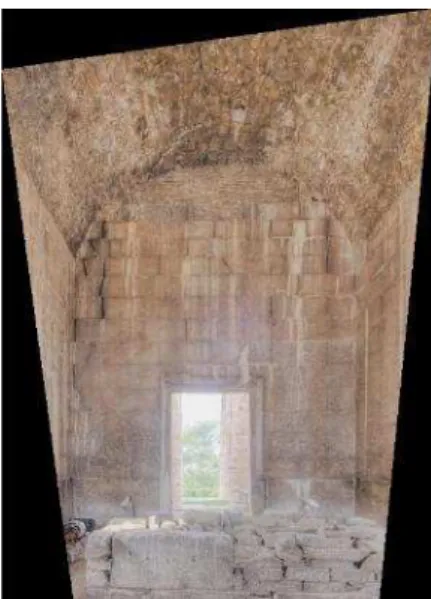
The results show that there is a discrepancy between the values that is mostly due to the precision that the user selects the points in the image. In the Implementation 3 (Fig.10), characteristic points could not be easily distinguished or found in the lower part of the image and as a consequence the accuracy of the EOPs estimation has been negatively influenced.

Figure 10: Implementation 3: Difficulty to detect characteristic points in the lower part of the image

In every consecutive iteration in the least squares process, an amount δxi is added in the approximation value xio _(xi’ ₌

xio+δxi). The iterations continue until the quantity δxi become smaller from a convergence criterion that has been set a priori. This convergence criterion is defined by the desired accuracy of the three linear (Xo, Yo, Zo) and three angular (ω, φ, κ) unknown elements, which are subsequently defined by the scale of the final output (e.g. scale of the orthoimage, defined by the user). As a consequence, it is obvious that the primary data must be measured with a better accuracy from the one that is wanted in the final output. Several attempts of selecting coordinates either in the image or in the point cloud showed that a more careful selection of the points by the user, affected significantly the accuracy of the estimated parameters.

3.4 Resulting Orthophotos

From the EOPs calculation, we concluded that the

Implementation 2 presented the best accuracy and as a

ˆ s o2

ˆ

s

ˆ

s

s

ˆ

s

ˆ

consequence that image was used for the orthophoto production (Fig.10). In order to assess the final output, distances between characteristic points were measured in the final georeferenced orthoimage and compared with the respective distances that derived from the geodetically measured points. For a scale of 1:50 of the final output, the results between the compared distances showed an error of approximately 22 mm, which is more than the maximum permitted value (12.5 mm). This error occurred due to the difficulty to identify characteristic points in the 3D point cloud and in the image respectively. Moreover, the density of the 3D point cloud led to a poor radiometric and geometric image quality. An attempt to produce an orthophoto with a scale of 1:100, led to better results as the error of the measured distances in the image were calculated around 10mm, while the expected maximum error for that specific scale is 25 mm.

Figure 11: Left: Oblique image of the east interior entrance that used in the algorithm. Right: The produced orthophoto

3.5 2D Rectification -Results

A practical implementation of the Rectification algorithm was conducted, using the digital image of the west interior side of the temple (Fig.9). The entrance that is shown in the image can be considered flat and also a slight tilt is presented in regard to the horizontal plane. Applying two different rotations to the geodetic coordinates a projection plane parallel to the main plane of the object is created. Least squares estimation process is taken place to evaluate the eight parameters of the transformation and through them the final rectified image is produced (Fig.12). The coordinates of three points in the object (Fig.13) were measured with a Total Station and those values were used to evaluate the accuracy of the final output. Three distances between those points were measured in the final image and were compared with the respective distances derived from the geodetically calculated coordinates. The differences are seen in Table 2 and the maximum difference reaches 0.55 cm, succeeding a value much smaller than the desired accuracy, which is 1.25 cm (scale of final object 1:50).

The final image was also compared with the results derived from another software called MPT (Matlab Photogrammetric Toolbox) that was built by Kalisperakis et al. (2006). The two final rectified images were compared by measuring characteristic distances in both images as well as the parameters of the transformation that derived from each case. All the comparisons showed insignificant differences.

Figure 8: Final georefenced image through rectification

Figure 9: The three geodetically measured points

r12(mm) r13(mm) r23(mm)

-5.5 -4.6 -3.9

Table 2: Differences between measured distances in the final georefenced image and distances that derived from

geodetically calculated coordinates

4. CONCLUSIONS

4.1 Sources of Error

space and relate them to the respective 2D points on the image. The poor edge definition of the point cloud can lead to the selection of slightly shifted points and subsequently to the increase of the total error.Additionally, in cases of simple objects with no vivid texture there is a difficulty in detecting enough characteristic points in both the image and the point cloud. This could result in a limited number or unevenly distributed GCP's, affecting significantly the photogrammetric procedures. On the other hand, a main plane cannot be easily defined on objects with vivid texture, hindering the rotation of the geodetic coordinates system. Finally and as mentioned before, the interpolation method that was implemented might insert additional errors in the production of the orthophoto. This error is highly dependent on the density of the point cloud.

The radiometric quality of the final products depends on the quality of the original image but also on the radiometric interpolation method. Apart from this, in the case of the orthophoto, the density of the point cloud and the selected interpolation method might also affect the final output, creating empty cells. The hole filling method improves significantly the radiometric quality of the orthophoto, however it is not suitable for an excessive number of black pixels.

4.2 Prerequisites

It is obvious that the proposed technique, although it is very beneficial in terms of cost, time and equipment, it requires some prerequisites in order to be effective. The problem that needs to be addressed is how to produce photogrammetric outputs with adequate accuracy for the documentation of monuments. To achieve this, every step of the procedure needs to be characterized by a better accuracy, e.g. one order of magnitude, from the required accuracy of the final result. Unfortunately, specific instructions of how to acquire the primary data (e.g. 3D point cloud, digital images) do not exist and the necessary fieldwork depends on the characteristics of the object under study. However, there are empirical guidelines that can provide an approximation of specifications. For instance, the scale of the primary image has to be approximately 3-8 times smaller from the scale of the final output and this gives an estimation of the distance H

between the camera and the object (H=c k). Images should be acquired with a calibrated camera and the average size of the ground sampling distance should not exceed the respective size on the orthophoto.

Regarding the proposed method, it is obvious that the density and the accuracy of the point cloud are the main determinants of the overall quality of the final outputs, especially in the case of the orthophoto. To confront the aforementioned sources of error the accuracy of the scans has to better that the size of the GSD of the final image. Usually for the documentation of monuments fine scale products are required and subsequently laser scanners of high accuracy must be usedWhat needs to become clear is that the scanner resolution but also the mean GSD of the collected images are the main determinants of the finest scale that can be achieved for the final products. However, depending on the desired product scale, the aforementioned characteristics along with the necessary equipment can and should be defined prior to the field work.

Hence, the proposed method requires careful planning so as to define the scanning step according to the desired scale of the final products. The point cloud must be dense enough in order to easily and accurately select ground control points but also to avoid an excessive number of empty pixels in the final

orthophoto.

Obviously, if the initial data are carefully collected and according to the scale of the final output the sources of errors can be minimised and accuracies equivalent to the geodetic measurements can be achieved. Undoubtedly, improvements are required but this attempt proves that the limitation of geodetic measurements in such a precise procedure as the documentation of monuments is possible and has the potential of producing accurate results under certain conditions.

4.3 Further Improvements

A summary of further possible improvements of the procedure is shown below.

 Non-determination of a main plane of the object.

There is a weakness in the algorithm when the ground coordinate system is not rotated to a photogrammetric one. In the least squares process the collinearity equations failed to converge to an accurate solution due to the existence of angles (ω, φ or κ) greater than approximately 40 degrees. In order to rotate the system the user has to define two points in the main plane of the object. That means that complex objects (i.e. statues) are excluded from the procedure, as it is not possible to define a main plane on them. Use of premarked targets in the object space may provide a solution.

 Optimisation of the algorithm’s run time

Although, many improvements have been done regarding the execution time for the orthophoto generation, further optimisations have to be considered for the resection algorithm, as the time increases significantly while the number of input points (object and image coordinates) getting bigger (i.e. more than 10 points).

 Automatic detection of ground control points

A significant step towards the overall automation of the described procedure is the automatic detection of ground control points. Using stereo-pair image, object coordinates can be estimated as well as the 3D reconstruction of the object (Karras, 2005).

 Usage of non-metric camera – Self calibration

A self-calibration routine can be included in the algorithm, if the user does not have prior knowledge of the interior orientation parameters of the camera (Georgopoulos & Natsis, 2008). In the implemented algorithm there is only the choice to exclude the interior parameters but with significant effects in the final accuracy.

5. REFERENCES

Abdel-Aziz, Y.I, Karara, H.M., 1971. Direct linear transformation from comparator coordinates into object-space coordinates. ASP Symp. on Close-Range

Photogrammetry, pp. 1-18.

Bartos, K., Pukanska, K.,Gajdosik, J., Krajnak, M., 2011, The issue of documentation of hardly accessible historical monuments by using of photogrammetry and laser scanner techniques, Proceedings of XXIII CIPA Symposium, September 2011, Prague, Czech Republic.

Chen, T., Shibasaki, R.S., 1998. Determination of camera’s orientation parameters based on line features. International

Archives of Photogrammetry and Remote Sensing, 32(5),

pp.23–28.

Cooper, M.A.R., Robson, S., 1996. Theory of close range photogrammetry. In: Atkinson, K. B. ed. 1996. Close-range

Photogrammetry and Machine Vision, Caithness: Whittles

Publishing, Ch.2.

Dulgerler, O.N., Gulec, S.A., Yakar , M., Yilmaz, H.M. , 2007, Importance of digital close-range photogrammetry in documentation of cultural heritage, Journal of Cultural

Heritage, 8, pp. 428-433.

Dallas, R.W.A., 1996, Architectural and Archaeological Photogrammetry, In: Atkinson, K. B. ed. 1996. Close-range

Photogrammetry and Machine Vision, Caithness: Whittles

Publishing, Ch.10.

El-Manadili Y., K. Novak, 1996. Precision Rectification of SPOT Imagery Using the Direct Linear Transformation Model , Photogrammetric Engineering & Remote Sensing, 62(1), pp. 67-72

Georgopoulos, A., Ioannidis, G., 2004. Photogrammetric and surveying methods for the geometric recording of archaeological monuments. Archaeological Surveys, FIG

Working Week Athens, Greece.

Georgopoulos, A., Natsis, S., 2008. A Simpler Method for Large Scale Digital Orthophoto Production, International Archives Of Photogrammetry Remote Sensing And Spatial

Information Sciences, 37(1), pp. 253-258

Griesbach, D., Reulke, R., Wehr, A., 2004, High Resolution Mapping Using CCD-line Camera and Laser Scanner with Integrated Position and Orientation System, International Archives Of Photogrammetry Remote Sensing And Spatial

Information Sciences, 35, pp. 506-511

Haddad, N.A., 2011. From ground surveying to 3D laser scanner: A review of techniques used for spatial documentation of historic sites. Journal of King Saud

University - Engineering Sciences, 23(2), pp.109–118.

Ji, Q., Costa, M. S., Haralick, R. M., & Shapiro, L. G., 2000. A robust linear least-squares estimation of camera exterior orientation using multiple geometric features. ISPRS Journal

of Photogrammetry and Remote Sensing, 55(2), pp. 75–93

Kaehler, M., Koch, M., 2009, Combining 3D Laser-Scanning and Close-Range Photogrammetry - An Approach to Exploit the Strength of Both Methods, Computer Applications to

Archaeology, Williamsburg, Virginia, USA, March 22-26.

Kalisperakis, I., Grammatkopoulos, L., Petsa, E. and Karras, G., 2006. An open-source educational software for basic photogrammetric tasks, Proc. International Symposium Modern Technologies, Education & Professional Practice in

Geodesy & Related Fields, Sofia, pp. 581-586.

Karras, G. Mountrakis, P. Patias, E. Petsa, 1998, Modeling Distortion of super-wide-angle lenses for Architectural and Archaeological applications. International Archives of

Photogrammetry & Remote Sensing, 32(5), pp. 570-573,

Hakodate, Japan.

Karras, G., 1998. Coordinates Linear Transformations in Photogrammetry, Lecture notes, SRSE, NTUA (In Greek).

Karras, G., 2005. Is it realistic to generate control points from a stereo pair?. Proceedings XX CIPA International

Symposium, Torino, pp. 399-402.

Krauss, K., 2003. Photogrammetry. Volume 1, Edition Τ (in Greek).

Mitka, B., Rzonca, A., 2009. Integration of photogrammetric and 3D laser scanning data as a flexible and effective approach for heritage documentation. In: International

Archives of Photogrammetry and Remote Sensing,

Commission V, ISPRS XXXVIII Congress, Trento, Italy.

Seedahmed, G.H., 2006. Direct retrieval of exterior orientation parameters using a 2-D projective transformation.

Photogrammetric Record, 21(115), pp.211–231.

Smith, M.J., Park, D.W.G., 2000. Absolute and exterior orientation using linear features. International Archives of

Photogrammetry and Remote Sensing, 33(B3), pp. 850–857.

U.N.E.S.C.O., 1972. Photogrammetry applied to the survey of Historic Monuments, of Sites and to Archaeology. UNESCO editions.

Valanis, A., Georgopoulos, A. Ioannidis, Ch., Tapinaki, S., 2009. High Resolution Textured Models for Engineering Applications. Proceedings XXII CIPA Symposium, October 11-15, 2009, Kyoto, Japan.

Wang, Y., 1992. A rigorous photogrammetric adjustment algorithm based on co-angularity condition. International

Archives of Photogrammetry and Remote Sensing, 29(5),

pp.195–202.

Yastikli, N., 2007, Documentation of cultural heritage using digital photogrammetry and laser scanning, Journal of