the Subtropical Northeast Atlantic
Carlos Ca´ceres*, Fernando Gonza´lez Taboada, Juan Ho¨fer, Ricardo Anado´n
Departamento de Biologı´a de Organismos y Sistemas, Universidad de Oviedo, Oviedo, Asturias, Spain
Abstract
Dilution experiments were performed to estimate phytoplankton growth and microzooplankton grazing rates during two Lagrangian surveys in inner and eastern locations of the Eastern North Atlantic Subtropical Gyre province (NAST-E). Our design included two phytoplankton size fractions (0.2–5mm and .5mm) and five depths, allowing us to characterize differences in growth and grazing rates between size fractions and depths, as well as to estimate vertically integrated measurements. Phytoplankton growth rates were high (0.11–1.60 d21), especially in the case of the large fraction. Grazing rates were also high (0.15–1.29 d21), suggesting high turnover rates within the phytoplankton community. The integrated balances between phytoplankton growth and grazing losses were close to zero, although deviations were detected at several depths. Also, O2supersaturation was observed up to 110 m depth during both Lagrangian surveys. These results add up to increased evidence indicating an autotrophic metabolic balance in oceanic subtropical gyres.
Citation:Ca´ceres C, Taboada FG, Ho¨fer J, Anado´n R (2013) Phytoplankton Growth and Microzooplankton Grazing in the Subtropical Northeast Atlantic. PLoS ONE 8(7): e69159. doi:10.1371/journal.pone.0069159
Editor:David L. Kirchman, University of Delaware, United States of America ReceivedNovember 14, 2012;AcceptedJune 11, 2013;PublishedJuly 23, 2013
Copyright:ß2013 Ca´ceres et al. This is an open-access article distributed under the terms of the Creative Commons Attribution License, which permits unrestricted use, distribution, and reproduction in any medium, provided the original author and source are credited.
Funding:This research has been supported by CARPOS (MEC, REN2003-09532-C03-03) and DOS MARES (CTM2010-21810-C03-03) projects. CC was supported by a FPU fellowship by MEC (AP2008-03658) and FGT by a FICYT ’’Severo Ochoa’’ fellowship (PCTI2006-09, Gobierno del Principado de Asturias). JH was supported by research contracts from CARPOS (MEC) and RADIAL (IEO- Universidad de Oviedo) projects. The funders had no role in study design, data collection and analysis, decision to publish, or preparation of the manuscript.
Competing Interests:The authors have declared that no competing interests exist. * E-mail: Carlos.l.caceres@gmail.com
Introduction
Oligotrophic subtropical oceans cover around 40% of the Earths surface and are currently expanding [1]. Nutrient concentrations are very low during most of the year mainly as a consequence of phytoplankton activity and vertical stratification [2]. For this reason, phytoplankton biomass is typically lower than in other marine environments, and there is a higher contribution of picophytoplankton to total phytoplankton biomass [3]. How-ever, these properties do not necessarily mean low phytoplankton growth rates, or low primary production: subtropical gyres resemble desserts in their low biomass, but regarding their growth rates they could be more similar to tropical forests [4].
There are a wide range of phytoplankton growth rate estimates (from,0.1 d21
, e.g.[5]; to more than 1 d21
, e.g.[4]), which surely arises from spatiotemporal heterogeneity [5], but maybe also from the lack of agreement between different measurement methods [6,7]. Hence, phytoplankton growth rates derived from primary production estimates based on the14C method [8] have frequently resulted in values near the lower range. In oligotrophic subtropical environments, high grazing rates [9], together with the release of dissolved organic carbon compounds [10], resulting in isotope cycling, might explain apparent low rates obtained with the14C method [11]. This is not a trivial matter since the magnitude of phytoplankton growth rates is a key feature to understand the functioning of these ecosystems and their role in biogeochemical cycles.
Oligotrophic subtropical gyres could sustain high phytoplankton growth rates if nutrient utilization by phytoplankton was coupled to nutrient regeneration [12]. In this case, a top-down regulation
of the phytoplankton community would prevail. Herbivores, mainly microzooplankton and nanozooplankton, would play an important role in maintaining high growth rates by controlling producers biomass [13], avoiding severe competition for nutrients, and by taking an active part in nutrient regeneration [14]. On the contrary, without herbivory, low phytoplankton growth rates would result due to severe nutrient limitation. In this case a bottom-up regulation of the phytoplankton community would prevail. Also, because the contribution of the biological pump [15] to net carbon sequestration depends on the balance between primary production and respiration, the role of subtropical gyres in atmospheric CO2regulation depends upon how the ecosystem functions, which is directly impacted by microzooplankton grazing activities.
differences in growth and grazing rates within the phytoplankton community.
Materials and Methods
Study Area and Survey
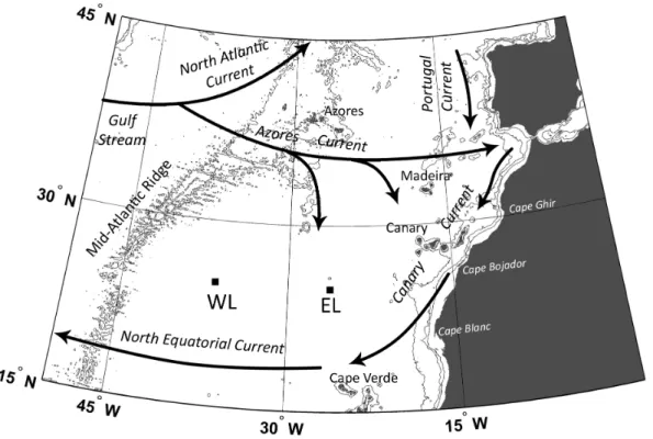
The study was conducted as part of the CARPOS project (Plankton and CARbon fluxes in Subtropical Oligotrophic environments: a Lagrangian approach) aboard the RV ‘Hespe´rides’. Dilution exper-iments were carried out in the context of two Lagrangian surveys located around 25uN, 36uW (WL) and 25uN, 26uW (EL) (Fig. 1), within the NAST-E province. Experiments during WL were performed between October 25th and 30th, 2006, while experi-ments during EL were conducted between November 15th and 20th, 2006. Experiments in each Lagrangian survey were conducted during five consecutive days. Only one experiment was performed at each depth each day. The Lagrangian survey presents some advantages including the possibility of working in the same water body for several days, which allowed us to perform dilution experiments at several depths over consecutive days. The water body was tracked with a buoy joined to a drogue installed at 25 m depth. We obtained relative current velocities by using an Acoustic Doppler Current Profiler (ADCP) installed at the buoys line, allowing us to estimate the deviation of the buoy with respect to the tracked water body (see Aranguren et al. [21] for further details).
Water Column Properties
Vertical distributions of temperature, salinity, fluorescence, dissolved oxygen concentration (mg O2L
–1
) and the percentage of oxygen saturation (O2sat,%) were obtained using a SBE-19 CTD, equipped with a SeaPoint fluorometer and a SeaBird SBE-43 oxygen meter. These variables were recorded between three and
seven times per day. Water samples were obtained with a rosette equipped with 24 Niskin bottles of 12 L. Winklers method was employed to calibrate the SBE-43 oxygen sensor (R2= 0.96). The depth of the photic layer (depth at which photosynthetic active radiation was 1% of the surface irradiance) was determinedin situ
from radiometer data. Nutrient analyses (NO3–, NO2–and PO4–) were carried out from water collected between one and six times per day in polystyrene tubes, which were immediately frozen and preserved at 280uC for analysis using a Technicon AAII autoanalyser [22]. Only the data obtained on the days when dilution experiments were performed were retained for analysis.
Plankton Abundance
Size-fractionated Chl a concentrations (mg Chl a m–3) were determined from initial samples of the dilution experiments, which were performed at 10, 30, 50 and 80 m depth, and at the DCM. Only one depth was sampled each day, corresponding to the depth of the dilution experiment for that day. We processed two 1000 ml samples from each depth. Samples were sequentially filtered through 5mm and 0.2mm pore diameter polycarbonate filters, which were arranged in line filter funnels. The filters were frozen and stored 24 h in dark. They were subsequently submerged in 90% acetone for 8–12 h. Chl a concentration was determined using the non-acidification technique [23] with a Turner Designs (TD-700) fluorometer calibrated with pure Chla. From the two samples measured at each depth, we estimated the mean and the standard deviation (S.D.) of the Chl a concentration. We used those mean Chlaestimates to calculate the integrated Chlaup to 125 m depth by trapezoidal integration. Total Chlaconcentration at each depth was determined by adding the two size-fractionated measurements.
Approximated carbon biomass was derived from size-fraction-ated Chladata applying the C: Chlaratios presented by Maran˜o´n
Figure 1. Map showing the study area and the location of the surveys.Two Lagrangian surveys were conducted during the CARPOS cruise near the center of the subtropical gyre,i.e.the West Lagrangian (WL), and near the eastern boundary,i.e.the East Lagrangian (EL).
et al. [24] for the North Atlantic Subtropical gyre: they were 103 at the upper mixed layer (UML) and 21 at the deep chlorophyll maximum (DCM) for the,2mm phytoplankton fraction. Values for .2mm phytoplankton were 247 at the UML and 60 at the DCM. C: Chlaratios for phytoplankton ,2mm were used for phytoplankton,5mm, while values for algae.2mm were used for the algae .5mm. Note that this is a conservative approach since C: Chlaratios usually increase with the size of phytoplank-ton. Ratios for the UML were used from the surface up to the beginning of the DCM layer, defined as the depth where Chla
concentration was half of the DCM. The DCM was determined after examining SeaPoint fluorometer profiles. Finally, the relative abundance of diatoms, dinoflagellates, ciliates, radiolarians and copepod nauplii was estimated during EL at the same depths in which dilution experiments were performed. Samples (2.0 L) were processed using a FlowCam [25] configured in the autoImaging mode, with a 100mm flow cell and a 10x objective.
The picophytoplankton community in EL was also analyzed by flow cytometry (FCM). Samples were fixed with a 1% parafor-maldehyde plus 0.05% glutaraldehyde solution and stored at 280uC until analysis. A FacScan flow cytometer (Becton, Dickinson and Company) was used. Phytoplankton were grouped and enumerated according to side-scattered light (SSC), orange fluorescence (FL2, 585621 nm) and red fluorescence signal (FL3, .650 nm). Samples were run at a flow rate between 38.6 and 43.2mL min21
. Three groups were identified: Prochlorococcus,
Synechococcusand picoeukaryotes. Cell abundances (mean6S.D.) were obtained from the four initial undiluted samples analyzed at each depth (two from carboys with nutrient addition and another two from carboys without nutrient addition). We estimated the amount of biomass (carbon) in each cell detected by the flow cytometer using the conversion factors reported by Zubkov et al. [26] forProchlorococcus(32 fg C cell21
) andSynechococcus(103 fg C cell21
), and Zubkov et al. [27] for picoeukaryotes (1.5 pg C cell21 ). We integrated these average biomass values from each experi-mental depth over all depths sampled down to 125 m in each Lagrangian survey to estimate the integrated C biomass of each picoplankton group.
The Dilution Method
The dilution method provides estimates of phytoplankton growth rate (m, d21
) and phytoplankton mortality rate (m, d21
). The basis of the method is to uncouple phytoplankton growth rate from microzooplankton grazing by the addition of filtered seawater [16].The addition of filtered seawater dilutes the sample, reducing the encounter rates between phytoplankton and grazers and consequently phytoplankton grazing mortality (m) in an amount assumed to be linearly related to the dilution factor (f). Then, linear regression analysis of phytoplankton apparent growth rate (r) againstfyields a slope and an intercept which corresponds to the rates of microzooplankton grazing and phytoplankton growth (m), respectively.
r~m{mf :
The balance between phytoplankton production and consump-tion is estimated as the difference between m and m (i.e., m-m balance, d21
). It can be expressed in relative values, as the percentage of production grazed (% pNPP), dividingmbym.
Apparent phytoplankton growth rate is estimated assuming an exponential growth model during the incubation:
Pt~P0ert?r~1
tln Pt P0
where P0 and Pt are observed population abundance (
Prochlo-rococcuscells ml21) or biomass (mg C m23, calculated from size fractionated Chl a measurements) at initial and final times, respectively.
Different nutrient availabilities along dilution treatments could makemchange with the dilution, and cause non-linearities in the dilution relationship to occur. This problem can be avoided by providing an appropriate mixture of inorganic nutrients [16]. We followed this recommendation in the first experiments, conducted at 80 m depth and DCM in WL. Phytoplankton apparent growth rates were compared between treatments with added nutrients (rn)
and no added nutrients (r0). Assuming that mortality rates were
unaffected by the nutrient additions, these treatments allowed the calculation of growth rates (m0) in natural seawater [28]:
m0~r100%zm
where r100% is the net growth rate observed in non-enriched
undiluted containers. However, in those two first experiments, we did not find any effect of nutrient addition on phytoplankton net growth rates in the undiluted containers, which contain the higher biomass and possibilities of nutrient effect. Thus, in the rest of experiments (except at 50 m depth) nutrients were only added to two undiluted containers to check possible effects.
Particulate net primary production (pNPP, mg C m23 d21
) and grazing losses (G, mg C m23
d21
) were estimated using C: Chla
ratios (see the subsection Plankton abundance) and the equations proposed by Landry et al. [29] based on Frost [30]:
pNPP~m0Pm G~m Pm
Pm~ 1
t{t0 ðt
t0
P0eðm{mÞxdx
?
t0~0
Pm~P0(e m{m
ð Þt1)
(m0)t
wherePmis the mean concentration of phytoplankton (mg C m23)
during each experiment.
We estimated net changes of Chlain the sea at the same depths and times of the dilution experiments (less than 2h of difference) to check their relationship withm-mbalances (considering both size fractions together) obtained from dilution experiments. To do that, we used CTD fluorescence data near the initial and final times of each dilution experiment and assumed an exponential phyto-plankton growth model. Data below the UML were not included in the analysis to avoid the influence of processes like vertical displacement of the DCM that might affect net changes in Chla
concentration and hamper the detection of any relationship with m-mbalance.
changes in Chlaconcentrations (Fig. 2, see also [21]). Hence,h-S plots from different vertical profiles conducted during the days in which dilution experiments were performed overlapped quite well, except at the base of the thermocline, suggesting a good tracking of the water body (Fig. 3). Integrals (0–125 m) of pNPP, G, and pNPP-G were determined using the trapezoidal method. Then, these integrals were divided by phytoplankton carbon biomass, resulting in integrated values for m, m, and m-m, which has the effect of accounting for differences in biomass between size fractions and depths.
Experimental Setup, Sampling and Analysis Procedure Water for the dilution experiments was collected at five depths: 10, 30, 50, 80 m and at the DCM (115 m in WL and 110 m in EL). Each day, water from one depth was collected at 4:30–5:00 h GMT, always before dawn, using two 30 L Niskin bottles. Lights onboard were turned off during sampling, except for minimal safety requirements. Carboys, containers, capsule filters and auxiliary pipes were stored in 10% HCl-Milli-Q water between experiments, and rinsed sequentially with Milli-Q water and 0.2mm filtered seawater immediately before use. Capsules were changed every four experiments. We checked that water filtration did not increase the inorganic nitrogen and phosphorous concentrations. From one 30 L Niskin bottle, 25 L were gently transferred to a polycarbonate carboy fully wrapped in black plastic, using silicone tubing fitted with 200mm mesh to eliminate mesozooplankton. At the same time, another 25 L from the other
Niskin bottle were filtered through a Gelman SuporCap 100 capsule filter (0.2mm) to obtain the water added to diluted treatments. Water filtered through the capsules showed undetect-able Chlaconcentrations and negligible numbers of fluorescent particles when they were examined by FCM. Unfiltered, prescreened seawater was gently mixed with filtered seawater in 2.3 L Nalgene polycarbonate containers to obtain two replicated dilutions withf =0.25, 0.50, and 0.75. Replicated dilutions with
f =1 (with and without nutrient enrichment) were obtained by filling containers with unfiltered prescreened seawater. Initial Chl
aconcentration for each treatment were calculated as the product of the measured initial Chl a concentration at f= 1 and the different dilution factors.
The nutrient mixture added to the enriched treatments resulted in a final concentration of 1mM ammonium (NH4Cl), 0.5mM phosphate (H3PO4), 5 nM iron (FeSO4) and 0.1 nM manganese (MnSO4). Powder-free plastic gloves were used during all operations. Containers were kept in dark during the whole process until placed in on-deck incubators. Incubations started always 1.5 h after water collection and lasted approximately 21 h. Blue sheets of light filters were combined to simulate in-situ light intensity and spectra. When necessary, the combination of light filters was corrected after light measurements in the morning, thus correcting possible small shifts in the amount of irradiance reaching the different depths. Temperature was kept within 60.5oC ofin situtemperature by connecting a cooler and a heater to two thermostats. Water inside the incubator was homogenized Figure 2. Properties of the water column during dilution experiments.Vertical profiles of temperature (A, H), salinity (B, I), fluorescence (C, J), oxygen (D, K), O2saturation (E, L), nitrate plus nitrite (F, M) and phosphate (G, N) in the upper 200 m during dilution experiments in WL (top) and EL
(bottom). Each grey line represents a different profile. Grey points represent nutrient concentrations. An additive transparency factor was applied to appreciate the agreement between values, being color intensity proportional to the number of overlapped lines or points, respectively. Black solid lines and points stand for average values.
by a submersible pump, which also shook gently the containers [20].
Samples taken at timest0andtfwere also examined underin vivo
FlowCam and a stereo microscope (Leica Z12.5) to check for potential damages to microzooplankton during sample gathering and handling, and during the incubations. FlowCam images showed undamaged microzooplankters, suggesting a reduced damage to microzooplankton during sample handling and during incubations. Samples processed by flow cytometry during EL were taken from each container at times t0and tf. We only show the
results of dilution experiments for Prochlorococcus because of the generally low R2 values and high standard errors of regressions obtained for the other groups. A solution of 1mm fluorescent latex beads was added to each sample and used as a standard to estimate relative FL3 signals ofProchlorococcus.We used these data as proxies for chlorophyll fluorescence changes during the incubations, as these changes would affect Chl a-based growth rate estimates. Statistical analyses were conducted using Statistica
8 and R [31] softwares. Graphs were plotted using Grapher software and the R packageggplot2[32].
Results
Oceanographic Conditions
Temperature and salinity in WL were warmer and saltier than in EL, and the thermocline and halocline were deeper in EL (Fig. 2A, B, H, I). As a result, the upper mixed layer was also deeper in EL. The depth of the photic layer was around 105 m during both Lagrangian surveys. Nutrient concentrations were very low in the photic layer in both Lagrangians (NO32 plus NO22 ,0.3mM and PO42 ,20 nM). There was a sharp nutricline at 140 m depth in WL and at 130 m depth in EL (Fig. 2F, G, M, N). The DCM was located at 115 m and 110 m depth in WL and EL respectively (Fig. 2C, J). Average oxygen saturation was above 100% down to 108 m in WL and down to 113 m depth in EL (Fig. 2E and 2L). These levels of O2saturation imply a net autotrophic balance since the last mixing event, when atmosphere and ocean O2 concentrations were equilibrated. Indeed, maximum values were found at 73 and 74 m depth in WL and EL, respectively. Oxygen concentration profiles followed similar patterns (Fig. 2D and 2K).
Temporal variation of physical-chemical variables was in general low within each Lagrangian survey, suggesting that we did indeed sample the same parcel of water over the 5 day survey (Fig 2, 3; see Aranguren et al. [21] for further details). A greater scatter of h-S pairs was found between isotherms 22.5uC and 20.75uC in WL (located around 77 m and 137 m depth, respectively) and between isotherms 22.65uC and 19.85uC in EL (located around 77 m and 138 m depth, respectively) (Fig. 3). This was probably caused by turbulent mixing promoted by Kelvin-Helmholtz instability associated to internal waves, and by salt fingers (see Thorpe [33]).
Plankton Abundance
Total integrated phytoplankton biomass was higher in EL than in WL, although if biomasses are expressed in C units values are similar (Table 1). Small phytoplankton integrated biomass was higher than the biomass of the large size fraction in both Lagrangian surveys (Table 1), although these differences diminish if biomasses are expressed in C units due to the higher C:Chla
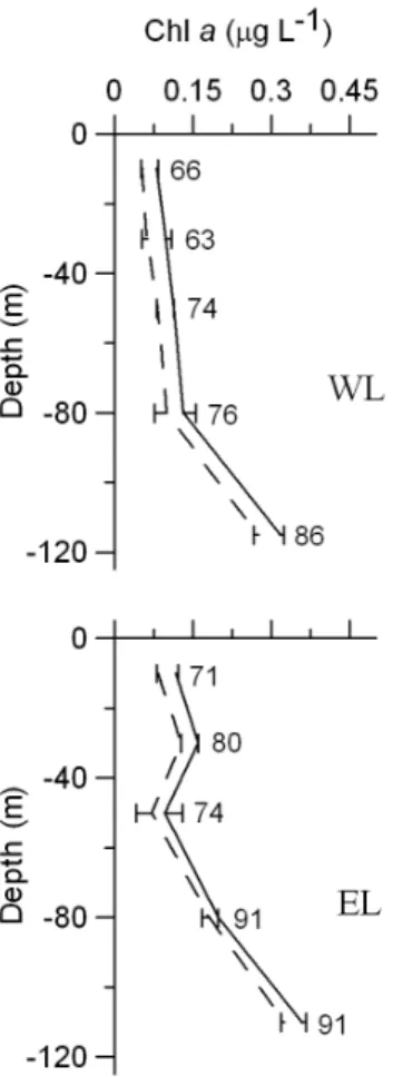
ratios of the large size fraction. The contribution of small phytoplankton to total Chlabiomass was higher near the DCM (Fig. 4). The picophytoplankton community in EL was numerically dominated by Prochlorococcus, with abundances two orders of magnitude higher than Synechococcusand picoeukaryotes (Fig. 5). Both groups of cyanobacteria followed a similar depth distribution pattern, with lower abundances at the DCM. In contrast, picoeukaryotes were slightly more abundant at the DCM.
Prochlorococcuswas also dominant in terms of integrated C biomass (633 mg C m22
), followed by picoeukaryotes (139 mg C m22 ) and
Synechococcus(16 mg C m22). Maximum abundances of diatoms, ciliates, radiolarians and copepod nauplii were found around 80 m depth in EL, where we also found a relative maximum abundance of dinoflagellates.
Dilution Experiments
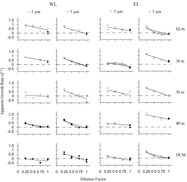
Phytoplankton apparent growth rates increased linearly with the dilution factor in most of the experiments. However, in six experiments out of 20, the relationship significantly improved by fitting a quadratic function (p,0.05, see fig. 6), although explained variances by simple linear regression were quite high in all those cases (R2.0.53). Integrated phytoplankton growth and Figure 3.h-S diagrams during dilution experiments.h-S plots
obtained from all the potential temperature (h) andSmeasurements conducted in the upper 200 m during dilution experiments in WL (top) and EL (bottom). The color intensity of the dots indicates the depth associated to eachh-Spair. Black lines are isopycnals. Numbers above
them point out sigma-theta values (sh= potential density21000 Kg m23). Dotted lines are isotherms between whichh-Splots dispersion
was higher.
microzooplankton grazing rates obtained in both Lagrangian surveys were high and similar (Table 2), suggesting a similar global functioning of the ecosystem in the two areas of study. Nevertheless, rates in WL and EL were different at some depths (Table 3). Regarding the comparison between phytoplankton size fractions, integrated phytoplankton growth and microzooplankton grazing rates were lower for the small phytoplankton fraction (Table 2). Hence, rates of the small phytoplankton size fraction
were similar or lower than the rates of the large fraction at all the depths analyzed (Table 3). Differences in growth rates between both phytoplankton size fractions were high below the UML in the two Lagrangian surveys, coinciding with the maximum phyto-plankton growth rates detected for the large phytophyto-plankton size fraction (Table 3).
Phytoplankton growth was not nutrient-limited in the experi-ments. Median phytoplankton growth rates obtained in nutrient addition treatments were indistinguishable from median phyto-plankton growth rates without added nutrients in the case of small (Wilcoxon matched pairs test,p =0.12,n =8) and large (Wilcoxon matched pairs test,p= 0.67,n =8) fractions. The ratios between phytoplankton growth rates without and with added nutrients (m0:
mn), were in general close to one (Table 3).
We obtained a very good relationship between m-m balances estimated from dilution experiments and net sea Chlachanges (data not shown;R2= 0.71, n = 6), providing further support to our experimental balances and rates. The totalm-mintegrated balance was close to zero in WL (Table 2). The integrated balance for Figure 4. Vertical profiles of Chlaconcentration up to the DCM
during dilution experiments in WL and EL.Solid lines stand for total Chlaaverage values. Dashed lines indicate average Chla,5mm. Horizontal bars represent6S.D. Numbers point out the percentage of Chla,5mm.
doi:10.1371/journal.pone.0069159.g004
Figure 5. Picophytoplankton abundance during dilution ex-periments in EL. Vertical profiles of Prochlorococcus (rectangles),
Synechococcus(circles) and picoeukaryotes (triangles) mean abundanc-es up to the DCM. Symbols also point out sampling depths. Horizontal bars represent6S.D. The 105cells mL21scale is forProchlorococcus,
whereasSynechococcusand picoekaryotes scale is 103cells mL21.
doi:10.1371/journal.pone.0069159.g005
Table 1.Phytoplankton integrated biomass in the water column during our experiments.
Site Size fraction (mm) Biomass (mg Chlam22) % Chla,5 Biomass (mg C m22) % C,5
WL ,5 15.19 78 801 52
.5 4.23 724
total 19.42 1525
EL ,5 20.83 87 970 65
.5 3.26 531
total 24.09 1501
Carbon based measurements were estimated using the C:Chlaratios reported by Maran˜o´n et al. 2007 (see Methods). WL and EL refer to the West and East Lagrangian, respectively (see Figure 1). % Chla,5: Contribution of phytoplankton Chlabiomass,5mm to the total Chlabiomass. % C,5: Contribution of phytoplankton C biomass,5mm to the total C biomass.
small phytoplankton was slightly positive, mainly due to the positive balance in the UML (Fig. 7). On the contrary, the integrated balance of large phytoplankton was slightly negative (Table 2), with positive values only around 80 m depth (Table 3, Fig. 7). The % pNPP consumed ranged between 61% and 136% for small phytoplankton and between 93% and 137% for large phytoplankton. Totalm-mintegrated balance was also balanced in EL, being them-mintegrated balances of both phytoplankton size fractions close to zero too (Table 2). The % pNPP grazed ranged between 53% and 187% for small phytoplantkon and between 45% and 129% in the case of the large fraction (Table 3). Them-m balance was positive at 80 m depth, near the maximum % O2
saturation, in both Lagrangians and for both phytoplankton size fractions.
Prochlorococcus growth rates at EL were nearly constant in the UML and relatively low (0.2 d21), reaching maximum and lowest values at 80 m depth and DCM, respectively (Fig. 8; Table 4). Grazing rates were also maximum at 80 m depth; nevertheless they changed along the UML (Table 4). In all the experiments analyzed, relationship between dilution factor and
nutrients were detected (Wilcoxon matched pairs test, p= 0.86,
n= 9).
Initial and final relative FL3 signals of Prochlorococcus were different (Sign test, p,0.001, n= 39). Relative FL3 increased during incubations at all depths except at the DCM. Differences between initial and final relative SSC, an indicative of cell size, were also observed (Wilcoxon matched pairs test, p= 0.003,
n =39) and followed a similar pattern as relative FL3 signal, although the magnitude of the changes was lower.
Discussion
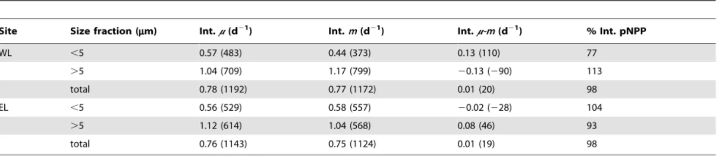
Dilution experiments were performed to assess ecosystem functioning and phytoplankton productivity in the eastern border and near the center of the North Atlantic Subtropical gyre. Despite the low nutrient concentrations, chlorophyll-based phyto-plankton growth and grazing rates were high, suggesting a very dynamic ecosystem similar to the proposed by Goldman et al. [12]. In the following, we discuss the operation of the microbial community taking into account the high phytoplankton growth Table 2.Integratedm,mandm-mbalance (d21) for both phytoplankton size fractions and Lagrangians.
Site Size fraction (mm) Int.m(d21) Int.m(d21) Int.m-m(d21) % Int. pNPP
WL ,5 0.57 (483) 0.44 (373) 0.13 (110) 77
.5 1.04 (709) 1.17 (799) 20.13 (290) 113
total 0.78 (1192) 0.77 (1172) 0.01 (20) 98
EL ,5 0.56 (529) 0.58 (557) 20.02 (228) 104
.5 1.12 (614) 1.04 (568) 0.08 (46) 93
total 0.76 (1143) 0.75 (1124) 0.01 (19) 98
In brackets besides each rate integral are their associated integrated pNPP, G and pNPP-G balances (mg C m22d21). The final column (% Int. pNPP) indicates the
percentage of phytoplankton grazed in the upper 125 m of the water column. doi:10.1371/journal.pone.0069159.t002
Table 3.Estimated growth and grazing rates for small (,5mm) and large (.5mm) phytoplankton size fractions.
Site
Depth (m)
Size fraction
(mm) mn±SE (d21) m0±SE (d21) m0:mn m±SE (d21) r
m-mbalance
(d21) % pNPP
WL 210 ,5 0.8 1.1060.17 1.38 0.7560.25 0.78* 0.35 68
210 .5 0.99 1.0360.10 1.04 1.0860.14 0.96** 20.05 105
230 ,5 0.87 0.9960.05 1.14 0.6060.07 0.99** 0.39 61
230 .5 1.12 1.0160.07 0.9 1.2260.10 0.98** 20.21 121
250 ,5 0.1160.20 0.1560.26 0.23 20.04 136
250 .5 0.9460.27 1.2960.35 0.79** 20.35 137
280 ,5 0.5660.08 0.66 1.18 0.5660.12 0.91** 0.1 85
280 .5 1.0060.16 1.21 1.21 1.1260.23 0.89** 0.09 93
2115 ,5 0.0060.28 0.22 0.2660.37 0.33 20.04 118
2115 .5 0.8460.16 0.95 1.13 1.0760.23 0.89** 20.12 113
EL 210 ,5 0.83 0.7560.18 0.9 0.5060.28 0.62 0.25 67
210 .5 0.8 0.7760.20 0.96 0.9960.29 0.81** 20.22 129
230 ,5 0.21 0.3160.15 1.48 0.5860.22 0.73* 20.27 187
230 .5 1.45 1.3960.09 0.96 1.1160.13 0.97** 0.28 80
250 ,5 0.8460.20 0.7660.30 0.72* 0.08 90
250 .5 1.1760.07 1.2160.10 0.98** 20.04 103
280 ,5 0.31 0.4560.09 1.45 0.2460.14 0.61 0.21 53
280 .5 1.68 1.6060.14 0.95 0.7260.20 0.82** 0.88 45
2110 ,5 0.64 0.4560.05 0.7 0.8060.09 0.97** 20.35 178
2110 .5 0.93 0.8660.16 0.92 0.8860.24 0.84** 20.02 102
mn: phytoplankton growth rate estimated from treatments with added nutrients.m0: phytoplankton growth rate estimated from treatments with no nutrients added.m:
microzooplankton grazing rate.m-mbalance: balance betweenmandm. % pNPP: % Particulated net primary production grazed. SE: Standard error of regression
and grazing rates obtained. Also, we discuss the metabolic balance fromm-mbalances and the O2supersaturation found. In the first part of discussion following, we underline some of the caveats and uncertainties related to the methods employed.
Potential Caveats of the Dilution Technique
The dilution technique is based on some assumptions [16] that must be validated to obtain correct estimates of phytoplankton growth and grazing rates. One of these assumptions is that dilution does not affect the estimates of both rates. For instance, several studies discuss the possibility that nutrient availabilities change across dilution treatments [16,19]. Another possibility we are not able to reject is related to the potential effects of dilution on mixotrophy, especially considering their importance in oligotro-phic environments [34]. Indeed, mixotrophs could increase their content of Chl a with dilution to obtain organic carbon by photosynthesis, compensating for the reduction of C obtained by predation (see Arenovski et al. [35] and references therein). This possible response would overestimate the rates obtained. The quantification of this effect remains a challenge for future dilution experiment studies in oligotrophic waters.
The observed increase in relative FL3 and SSC inProchlorococcus
cells seems to be the result of a light-dark cycle [36], although we can not entirely discard the occurrence of photoacclimation
processes. The experiments lasted approximately 21 h, and they started at the end of the dark period, when a low percentage of cells are at the G2 phase (% G2), resulting in their FL3 and SSC relative signals being close to their daily minimum [37]. Then, it would be possible to detect an increase in those signals, especially if growth rates were high. Hence, we found a positive logarithmic correlation between m0 and the increase in the relative FL3
(R2= 0.99, n= 5) and SSC (R2= 0.67, n= 5) signals, despite
Prochlorococcus growth rates would have to be low when photo-acclimation occurs [38]. Therefore, the rise of those signals could mean the existence of a Prochlorococcus growth which was not detected. Thus, Prochlorococcus growth rates might be underesti-mated.
Phytoplankton Growth and Microzooplankton Grazing Rates
The low nutrient concentrations found in both locations contrasted with the high phytoplankton growth rates obtained. They would be promoted by the high micro and nanozooplankton Figure 7. Vertical profiles summarizing the results of dilution
experiments.Phytoplankton growth rates (black squares and lines), grazing rates (grey squares and lines) andm-mbalances (white squares
and black dashed lines) of both phytoplankton size fractions and Lagrangians. Squares also point out the depths at which dilution experiments were performed. Grey dashed lines indicate the zero value.
doi:10.1371/journal.pone.0069159.g007 Figure 8. Plots of dilution experiments based on
Prochloro-coccusabundances. Simple linear regressions between dilution factor andProchlorococcus apparent growth rate in EL.White dots: Prochlorococcus apparent growth rate in treatments without added nutrients. Black dots:Prochlorococcusapparent growth rates in nutrient added treatments. Dashed lines indicate apparent growth rate = 0.
grazing rates detected [12], previously reported by Quevedo et al. [20] in surface waters and in the DCM. On one hand, grazers diminish phytoplankton biomass relaxing competition for nutri-ents. At the same time, grazers also take an active part in nutrient regeneration, increasing the amount of nutrients available to phytoplankton cells [14]. High phytoplankton growth rates would also be promoted by a variety of mechanisms known to diminish nutrient consumption or to improve nutrient uptake, like mixotrophy [34], phytoplankton associations [39], N2 fixation [40] and other biochemical and physiological mechanisms [41,42]. Indeed we did not find differences in phytoplankton growth rates between treatments with and without nutrient enrichment, maybe because of the short incubation times. For all those reasons, the regulation of the system seems closer to a top-down control than to a bottom-up one during the time of study, although the low amount of nutrients available would influence phytoplankton community composition and its overall biomass.
Our integrated growth rates were within the range of values reported in other studies carried out in open ocean oligotrophic regions (e.g. [18,43,44]). Also, similar phytoplankton growth rates have been reported in the Subtropical Pacific using the 14C method [45,46], although the rates reported here were greater than most of the 14C estimates reported in the NAST-E region [47,48,49]. Consequently, our pNPP estimates were also higher. However, the 14C method could largely underestimate primary production in oligotrophic environments [11], and, consequently, phytoplankton growth rates obtained with this methodology. This underestimation could be partially caused by the use of small incubation bottles [50,51]. In addition, the high percentage of pNPP grazed, typical from tropical regions [9] and also observed in this study, could prevent the detection of a considerable amount of the fixed carbon. All these reasons make the existence of differences in production estimates between 14C method and other techniques possible (see Quay et al. [6]).
We obtained higher growth rates for the large phytoplankton fraction despite the assumed competitive advantage of small phytoplankton to exploit low nutrient concentrations waters [52]. Slightly higher metabolic rates for the large phytoplankton were also reached in these latitudes by using the 14C method [50], although similar [48], or even lower rates [49] were observed using the14C method too. McCarthy and Goldman [53] suggested the existence of microscale nutrient patches resulting from zooplank-ton excretion and degradation of particulate organic matter. The existence of such nutrient patches, and the response of algal flagellates to them, was subsequently proved [54,55,56]. Large phytoplankton could take advantage of those patches because they generally have higher maximum nutrient uptake rates [57] and
motilities [58]. In addition, the storage capacity and vertical migration of some groups of large phytoplankton like diatoms [59], dinoflagellates or cyanobacteria of the genus Trichodesmium[60], could provide an advantage to exploit the nutrient heterogeneity at the vertical scale too. In this way, we propose that the spatio-temporal variability of nutrient concentrations might explain the higher growth rates obtained for the large phytoplankton. As Polz et al. [61] proposed for bacteria, there could be two strategies followed by phytoplankton in oligotrophic environments: the passive oligotroph (‘‘SS strategist’’ according to Reynoldss scheme [58], ‘‘affinity adapted’’ in Sommers [62] scheme), mainly adopted by small phytoplankton (e. g. Prochlorococcus), exploiting the low background nutrient concentrations; and the ‘‘opportuni-troph’’, which might be the strategy adopted by most of the large phytoplankton fraction (e.g. some phytoflagellates or diatoms), exploiting the nutrient enriched environments at different spatiotemporal scales.
In general, the differences in growth between both fractions were higher below the UML, where large phytoplankton growth rates were the highest recorded. This observation was especially evident at 80 m depth, coinciding with the maximum O2 supersaturation. At 80 m depth in EL we found the maximum abundance of diatoms and a relative maximum of dinoflagellates too. The higher availability of nutrients resulting from turbulent mixing processes, together with vertical excursions to take up nutrients in enriched deeper waters [59], could result in higher growth rates for large phytoplankton, especially considering their higher photosynthetic efficiency under non-limiting conditions [63]. In addition, microzooplankton (ciliates, nauplii and meta-nauplii) abundances were also maxima at this layer in EL. These activities might enhance the formation of microscale nutrient patches and might consequently promote the advantage of ‘‘opportuni-trophs’’, providing further enhancement to the very high growth rates detected for the large phytoplankton.
Production-grazing Balances and Metabolic Balances The percentage of pNPP grazed was at some depths far from 100%, especially in EL. This would indicatem-mimbalances that might be related to predator-prey cycles. In both Lagrangian surveys, the depth around maximum O2saturation seemed to be a net production zone of phytoplankton biomass (positive particulate m-mbalances at 80 m depth from Chlaanalysis andProchlorococcus counts), while the DCM was a net consumption zone (negativem-m balances). However, without mixing events or other restoration processes, them-mimbalances would not persist for a long time: the high potential growth and grazing rates of protists [64] and the low carrying capacity of phytoplankton populations in oligotrophic Table 4.Estimated growth and grazing rates forProchlorococcusin EL.
Depth (m)
mn
(d21) m0±SE
(d21)
m0:mn
m±SE
(d21) r pN
PP
(103cells ml21d21) PG
(103cells ml21d21)
m-mbalance
(d21) %PP 55
210 0.17 0.2260.02 1.29 0.1260.03 0.90* 39 21.3 0.1
230 0.07 0.2360.06 3.29 0.1360.08 0.6 41.9 23.7 0.1 57
250 0.3 0.2260.09 0.73 0.2760.13 0.68 35.5 43.6 20.05 123
280 0.83 0.6760.08 0.81 0.3460.12 0.78* 115.1 58.4 0.33 51
2110 0.07 0.1260.06 1.71 0.160.09 0.53 9.2 7.7 0.02 83
mn:Prochlorococcusgrowth rate estimated from treatments with added nutrients.m0:Prochlorococcusgrowth rate estimated from treatments with no nutrients added.
m: microzooplankton grazing rate. pNPP: Particulate netProchlorococcusproduction.PG:Prochlorococcusgrazing losses.m-mbalance: balance betweenmandm.%PP:
subtropical gyres, would limit the duration of positive imbalances. At the same time, the low phytoplankton stocks would prevent long negative imbalances. According to this idea, the potential length and amplitude of the imbalances would be maximum in winter and early spring, when nutrient concentrations and phytoplankton carrying capacity is maximum, and they would attenuate in summer, when the strengthened stratification favors lower nutrient concentrations in the surface.
In spite of the imbalances detected for single depths, the integrated % pNPP grazed of small and large phytoplankton were close to 100%, except in the case of the small phytoplankton fraction in the WL. If both phytoplankton fractions are treated together, then the integrated % pNPPs were even closer to 100%, greater than the average 74.5% pNPP grazed reported for the open ocean [9]. Nevertheless, most dilution experiments analyzed in Calbet and Landry [9] were performed in the UML, where the % pNPP grazed is in general lower. Therefore, the coupled integratedm-mbalances for both Lagrangian surveys are the result of multiple compensated imbalances, increasing the coupling of the system with the size of the phytoplankton compartment.
The integratedm-mbalance reported could be approximated to a simultaneous metabolic balance (production- respiration) if i) grazing exerted by mesozooplankton is very low [65,66], and mesozooplankton respiration is supported by carbon ingested from zooplankton consumption, ultimately coming from phytoplankton; and ii) bacterial respiration is fully supported by organic carbon coming from organisms of the contemporary community [67],i.e.
eventually fixed by phytoplankton. Under these circumstances, even slightly negative integrated m-m balances might imply autotrophic metabolic balances, given that part of the consumed phytoplankton would be finally exported and not respired in the upper water column. Therefore, according to the obtained m-m balances, the water column analyzed would be slightly autotrophic during our experiments. Indeed, our results are within the confidence intervals reported to the net plankton metabolic balances during the same Lagragian surveys by using oxygen in vitro measurements [21]. On the other hand, assuming a 30% dark phytoplankton respiration of pNPP, and 18% of extracellular release (PER) of the carbon photoassimilated by phytoplankton [68], the integrated GPP would be at least 1.68 g C m22d21in the two study areas. This value is higher than the average
community respiration found in the photic layer of the NAST-E province obtained from oxygen experiments [24,69].
Regarding the metabolic balance during longer time periods, oxygen supersaturation up to around 110 m depth was observed during Lagrangian surveys and along the approximately 2600 Km transect carried out just before the Lagrangian surveys [70]. This implies an autotrophic metabolic balance too, although the observed O2 supersaturation could be partially caused by a temperature increase during spring and summer [71]. Other studies also reported oxygen saturation levels higher than 100% [24,72]. Furthermore, net oxygen production and supersaturation was observed at other subtropical oligotrophic regions [6,73,74], especially in summer and fall [75].
Despite the m-m balance and the high GPP and the O2 supersaturation found, most studies in the North Atlantic subtropical gyre report that net heterotrophic metabolic balance prevails [69,72,76]. These opposing situations could take place if net heterotrophic events were more common and longer than the autotrophic ones, which would be infrequent and brief, although they would allow O2 supersaturation [77]. However, the overestimation of respiration [78,79], or the probable underesti-mation of primary production estimates based on O2incubations [6,79,80], could produce the same results. If autotrophy is the common situation [74], subtropical gyres could be an important carbon sink.
Acknowledgments
We thank the crew and scientific CARPOS team on board R.V. Herspe´rides, especially J. Sostres and L. Viesca. A. Calvo-Dı´az kindly provided FCM calibrations, shared some FCM data and helped, together with L.A. Sua´rez and L. Dı´az, with FCM operation. J. Esca´nez and J. F. Domı´nguez (IEO Canarias) measured nutrient concentrations. R. Gonza´lez-Gil assisted with R software use. Comments by N.F. Weidberg, C. Lobo´n, E. Lo´pez and A. Rivera and five anonymous reviewers improved greatly the quality of this paper and are especially acknowledged.
Author Contributions
Conceived and designed the experiments: RA. Performed the experiments: FGT RA JH. Analyzed the data: CC FGT RA JH. Contributed reagents/ materials/analysis tools: CC FGT RA JH. Wrote the paper: CC RA FGT JH.
References
1. Polovina JJ, Howell EA, Abecassis M (2008) Ocean’s least productive waters are expanding. Geophysical Research Letters 35: L03618. doi:03610.01029/ 02007GL031745.
2. Mann KH, Lazier JRN (2006) Vertical Structure of the Open Ocean: Biology of the Mixed Layer. Dynamics of Marine Ecosystems. Third ed. Oxford: Blackwell Publishing. 68–117.
3. Teira E, Mourin˜o B, Maran˜o´n E, Pe´rez V, Pazo´ MJ, et al. (2005) Variability of chlorophyll and primary production in the Eastern North Atlantic Subtropical Gyre: potential factors affecting phytoplankton activity. Deep-Sea Research I 52: 569–588.
4. Sheldon AW (1984) Phytoplankton growth rates in the tropical ocean. Limnology and Oceanography 29: 1342–1346.
5. Maran˜on E, Holligan PM, Varela M, Mourin˜o B, Bale AJ (2000) Basin-scale variability of phytoplankton biomass, production and growth in the Atlantic Ocean. Deep-Sea Research I 47: 825–857.
6. Quay PD, Peacock C, Bjo¨rkman K, Karl DM (2010) Measuring primary production rates in the ocean: Enigmatic results between incubation and non-incubation methods at Station ALOHA. Global Biogeochemical Cycles 24: doi:10.1029/2009GB003665.
7. Marra J (2002) Approaches to the measurement of plankton production. In: Williams PJlB, Thomas DN, Reynolds CS, editors. Phytoplankton productivity. Oxford: Blackwell Science Ltd. 78–108.
8. Steemann-Nielsen E (1952) The use of radiative carbon (14C) for measuring organic production in the sea. Journal du Conseil pour lexploration de la Mer 18: 117–140.
9. Calbet A, Landry MR (2004) Phytoplankton growth, microzooplankton grazing, and carbon cycling in marine systems. Limnology and Oceanography 49: 51–57.
10. Karl DM, Hebel DV, Bjo¨rkman K, Letelier RM (1998) The role of dissolved organic matter release in the productivity of the oligotrophic North Pacific Ocean. Limnology and Oceanography 43: 1270–1286.
11. Peterson BJ (1980) Aquatic primary productivity and the14
C-CO2method: A history of the productivity problem. Annual Review of Ecology and Systematics 11: 359–385.
12. Goldman JC, McCarthy JJ, Peavey DG (1979) Growth rate influence on the chemical composition of phytoplankton in oceanic waters. Nature 279: 210–215. 13. Strom S (2002) Novel interactions between phytoplankton and microzooplank-ton: their influence on the coupling between growth and grazing rates in the sea. Antonie van Leeuwenhoek 480: 41–54.
14. Sterner RW (1986) Herbivores direct and indirect effects on algal populations. Science 231: 605–607.
15. Volk T, Hoffert MI (1985) Ocean carbon pumps: Analysis of relative strengths and efficiencies in ocean-driven atmospheric CO2changes. In: Sundquist ET, Broecker WS, editors. The carbon cycle and atmospheric CO2: Natural variations Archean to present. Washington, DC: AGU. 99–110.
16. Landry MR, Hassett RP (1982) Estimating the grazing impact of marine micro-zooplankton. Marine Biology 67: 283–288.
17. Longhurst A (2007) Ecological geography of the sea. London: Academic Press. 18. Stelfox-Widdicombe CE, Edwards ES, Burkill PH, Sleigh MA (2000) Microzooplankton grazing activity in the temperate and sub-tropical NE Atlantic: summer 1996. Marine Ecology Progress Series 208: 1–12. 19. Lessard EJ, Murrell MC (1998) Microzooplankton herbivory and phytoplankton
20. Quevedo M, Anado´n R (2001) Protist control of phytoplankton growth in the subtropical north-east Atlantic. Marine Ecology Progress Series 221: 29–38. 21. Aranguren-Gassis M, Serret P, Ferna´ndez E, Herrera JL, Domı´nguez JF, et al.
(2012) Balanced plankton net community metabolism in the oligotrophic North Atlantic subtropical gyre from Lagrangian observations. Deep-Sea Research I 68: 116–122.
22. Tre´guer P, Le Corre P (1975) Manuel d’analyse des sels nutritifs dans l’eau de mer (utilisation de l’AutoAnalyzer Technicon). Brest: Universite´ de Bretagne Occidentale.
23. Welschmeyer NA (1994) Fluorometric analysis of chlorophyll a in the presence of chlorophyll b and pheopigments. Limnology and Oceanography 39: 1985– 1992.
24. Maran˜o´n E, Pe´rez V, Ferna´ndez E, Anado´n R, Bode A, et al. (2007) Planktonic carbon budget in the eastern subtropical North Atlantic. Aquatic Microbial Ecology 48: 261–275.
25. Sieracki CK, Sieracki ME, Yentsch CS (1998) An imaging-in-flow system for automated analysis of marine microplankton. Marine Ecology Progress Series 168: 285–296.
26. Zubkov MV, Sleigh MA, Tarran GA, Burkill PH, Leakey RJG (1998) Picoplanktonic community structure on an Atlantic transect from 50uN to 50uS. Deep-Sea Research I 45: 1339–1355.
27. Zubkov MV, Sleigh MA, Burkill PH, Leakey RJG (2000) Picoplankton community structure on the Atlantic Meridional Transect: a comparison between seasons. Progress in Oceanography 45: 369–386.
28. Andersen T, Schartau AKL, Paasche E (1991) Quantifying external and internal nitrogen and phosphorus pools, as well as nitrogen and phosphorus supplied through remineralization, in coastal marine plankton by means of a dilution technique. Marine Ecology Progress Series 69: 67–80.
29. Landry MR, Constantinou J, Latasa M, Brown SL, Bidigare RR, et al. (2000) Biological response to iron fertilization in the eastern equatorial Pacific (IronEx II). III. Dynamics of phytoplankton growth and microzooplankton grazing. Marine Ecology Progress Series 201: 57–72.
30. Frost BW (1972) Effects of size and concentration of food particles on the feeding behavior of the marine planktonic copepodCalanus pacificus. Limnology and Oceanography 17: 805–815.
31. R Core Team (2013). R: A language and environment for statistical computing. R Foundation for Statistical Computing, Vienna, Austria. Available: http:// www.R-project.org/. Accessed 2013 Jun 6.
32. Wickham H (2009) ggplot2: Elegant graphics for data analysis. New York: Springer.
33. Thorpe SA (2007) Turbulence in the ocean pycnocline. An introduction to ocean turbulence. Cambridge: Cambridge University Press. 116–157. 34. Hartmann M, Grob C, Tarran GA, Martin AP, Burkill PH, et al. (2012)
Mixotrophic basis of Atlantic oligotrophic ecosystems. Proceedings of Natural Academics of Science 109: 5756–5760
35. Arenovski AL, Lim EL, A.Caron D (1995) Mixotrophic nanoplankton in oligotrophic surface waters of the Sargasso Sea may employ phagotrophy to obtain major nutrients. Journal of Plankton Research 17: 801–820. 36. Vaulot D, Marie D, Olson RJ, Chisholm SV (1995) Growth ofProchlorococcus, a
photosynthetic prokaryote, in the equatorial Pacific Ocean. Science 268: 1480– 1482.
37. Jacquet S, Partensky F, Marie D, Casotti R, Vaulot D (2001) Cell cycle regulation by light in Prochlorococcus strains. Applied and Environmental Microbiology 67: 782–790.
38. Bricaud A, Allali K, Morell A, Marie D, Veldhuis MJW, et al. (1999) Divinyl chlorophylla-specific absorption coefficients and absorption efficiency factors for
Prochlorococcus marinus: kinetics of photoacclimation. Marine Ecology Progress Series 188: 21–32.
39. Villareal TA, Brown CG, Brzezinski MA, Krause JW, Wilson C (2012) Summer diatom blooms in the North Pacific subtropical gyre:2008–2009. PLoS ONE 7: p. e33109
40. Karl D, Michaels A, Bergman B, Capone D, Carpenter E, et al. (2002) Dinitrogen fixation in the world’s oceans. Biogechemistry 57/58: 47–98. 41. VanMooy BAS, Fredricks HF, Pedler BE, Dyhrman ST, Karl DM, et al. (2009)
Phytoplankton in the ocean use non-phosphorus lipids in response to phosphorus scarcity. Nature 458: 69–72.
42. Bonachela JA, Raghib M, Levin SA (2011) Dynamic model of flexible phytoplankton nutrient uptake. Proceedings of Natural Academics of Science 108: 20633–20638.
43. Landry MR, Brown SL, Campbell L, Constantinou J, Liu H (1998) Spatial patterns in phytoplankton growth and microzooplankton grazing in the Arabian Sea during monsoon forcing. Deep-Sea Research II 45: 2353–2368. 44. Edwards ES, Burkill PH, Stelfox CE (1999) Zooplankton herbivory in the
Arabian Sea during and after the SW monsoon, 1994. Deep-Sea Research II 46: 843–863.
45. Laws EA, DiTuillo GR, Redalje DG (1987) High phytoplankton growth and production rates in the North Pacific subtropical gyre. Limnology and Oceanography 32: 905–918.
46. Laws EA, Redalje DG, Haas LW, Bienfang PK, Eppley RW, et al. (1984) High phytoplankton growth and production rates in oligotrophic Hawaiian coastal waters. Limnology and Oceanography 29: 1161–1169.
47. Maran˜o´n E (2005) Phytoplankton growth rates in the Atlantic subtropical gyres. Limnology and Oceanography 50: 299–310.
48. Pe´rez V, Ferna´ndez E, Maran˜o´n E, Mora´n XAG, Zubkov MV (2006) Vertical distribution of phytoplankton biomass, production and growth in the Atlantic subtropical gyre. Deep-Sea Research I 53: 1616–1634.
49. Moreno-Ostos E, Ferna´ndez A, Huete-Ortega M, Mourin˜o-Carballido B, Calvo-Dı´az A, et al. (2011) Size-fractionated phytoplankton biomass and production in the tropical Atlantic. Scientia Marina 75: 379–389.
50. Huete-Ortega M, Cermen˜o P, Calvo-Dı´az A, Maran˜o´n E (2011) Isometric size-scaling of metabolic rate and the size abundance distribution of phytoplankton. Proceedings of the Royal Society B 279: 1815–1823
51. Gieskes W, Kraay G, Baars M (1979) Current14
C methods for measuring primary production: Gross underestimates in oceanic waters. Netherlands Journal of Sea Research 13: 58–78.
52. Raven JA (1998) The twelfth Tansley Lecture. Small is beautiful: the picophytoplankton. Functional Ecology 12: 503–513.
53. McCarthy JJ, Goldman JC (1979) Nitrogenous nutrition of marine phytoplank-ton in nutrient-depleted waters. Science 203: 670–672.
54. Lehman JT, Scavia D (1982) Microscale patchiness of nutrients in plankton communities. Science 216: 729–730.
55. Seymour JR, Marcos, Stocker R (2009) Resource patch formation and exploitation throughout the marine microbial food web. The American Naturalist 173: E15–29.
56. Azam F, Malfatti F (2007) Microbial structuring of marine ecosystems. Nature Reviews Microbiology 5: 782–791.
57. Litchman E, Klausmeier CA, Schofield OM, Falkowski PG (2007) The role of functional traits and trade-offs in structuring phytoplankton communities: scaling from cellular to ecosystem level. Ecology Letters 10: 1170–1181. 58. Reynolds C (2006) The ecology of phytoplankton. New York: Cambridge
University Press.
59. Villareal TA, Altabet MA, Culver-Rymsza K (1993) Nitrogen transport by migrating diatom mats in the North Pacific Ocean. Nature 363: 709–712. 60. Letelier RM, Karl DM (1998)Trichodesmiumspp. physiology and nutrient fluxes
in the North Pacific subtropical gyre. Aquatic Microbial Ecology 15: 265–276. 61. Polz MF, Hunt DE, Preheim SP, Weinreich DM (2006) Patterns and mechanisms of genetic and phenotypic differentiation in marine microbes. Philosophical Transactions of the Royal Society 361: 2009–2021.
62. Sommer U (1984) The paradox of the plankton: Fluctuations of phosphorus availability maintain diversity of phytoplankton in flow-through cultures. Limnology and Oceanography 29: 633–636.
63. Cermen˜o P, Este´vez-Blanco P, Maran˜o´n E, Ferna´ndez E (2005) Maximum photosynthetic efficiency of size-fractionated phytoplankton assessed by 14
C uptake and fast repetition rate fluorometry. Limnology and Oceanography 50: 1438–1446.
64. Sherr EB, Sherr BF (2002) Significance of predation by protists in aquatic microbial food webs. Antonie van Leeuwenhoek 81: 293–308.
65. Huskin I, Anado´n R, Medina G, Head RN, Harris RP (2001) Mesozooplankton distribution and copepod grazing in the Subtropical Atlantic near Azores: Influence of mesoscale structures. Journal of Plankton Research 23: 671–691. 66. Isla JA, Llope M, Anado´n R (2004) Size-fractionated mesozooplankton biomass,
metabolism and grazing along a 50uN230uS transect of the Atlantic Ocean. Journal of Plankton Research 26: 1301–1313.
67. Robinson C (2008) Heterotrophic bacterial respiration. In: Kirchman DL, editor. Microbial Ecology of the oceans. Second ed. New Jersey: Jhon Wiley & Sons. 299–327.
68. Teira E, Pazo´ MJ, Quevedo M, Fuentes MV, Niell FX, et al. (2003) Rates of dissolved organic carbon production and bacterial activity in the eastern North Atlantic Subtropical Gyre during summer. Marine Ecology Progress Series 249: 53–67.
69. Duarte CM, Agustı´ S, Arı´stegui J, Gonza´lez N, Anado´n R (2001) Evidence for a heterotrophic subtropical northeast Atlantic. Limnology and Oceanography 46: 425–428.
70. Taboada FG, Gil RG, Ho¨fer J, Gonza´lez S, Anado´n R (2010)Trichodesmiumspp. population structure in the eastern North Atlantic subtropical gyre. Deep-Sea Research I 57: 65–77.
71. Emerson S, Stump C, Nicholson D (2008) Net biological oxygen production in the ocean: Remote in situ measurements of O2and N2in surface waters. Global Biogeochemical Cycles 22: GB3023.
72. Robinson C, Serret P, Tilstone G, Teira E, Zubkov MV, et al. (2002) Plankton respiration in the eastern Atlantic Ocean. Deep-Sea Research I 49: 787–813. 73. Nicholson D, Emerson S, Eriksen CC (2008) Net community production in the
deep euphotic zone of the subtropical North Pacific gyre from glider surveys. Limnology and Oceanography 53: 2226–2236.
74. Riser SC, Johnson KS (2008) Net production of oxygen in the subtropical ocean. Nature 451: 323–325.
75. Karl DM (2007) Microbial oceanography: paradigms, processes and promise. Nature Reviews Microbiology 5: 759–769.
76. Aranguren-Gassis M, Serret P, Ferna´ndez E, Herrera JL, Domı´nguez JF, et al. (2011) Production and respiration control the marine microbial metabolic balance in the eastern North Atlantic subtropical gyre. Deep-Sea Research I 58: 768–775.
77. Karl DM, Laws EA, Morris P, Williams PJleB, Emerson S (2003) Metabolic balance of the open sea. Nature 426: 32.
seawater by the precision Winkler Method. Applied and Environmental Microbiology 60: 328–332.
79. Calvo-Dı´az A, Dı´az-Pe´rez L, Sua´rez LA´ , Mora´n XAG, Teira E, et al. (2011) Decrease in the autotrophic-to-heterotrophic biomass ratio of picoplankton in oligotrophic marine waters due to bottle enclosure. Applied and Environmental Microbiology 77: 5739–5746.