www.hydrol-earth-syst-sci.net/20/2899/2016/ doi:10.5194/hess-20-2899-2016
© Author(s) 2016. CC Attribution 3.0 License.
On the propagation of diel signals in river networks using analytic
solutions of flow equations
Morgan Fonley1,2,4, Ricardo Mantilla2,3, Scott J. Small2, and Rodica Curtu1 1Department of Mathematics, University of Iowa, Iowa City, Iowa, USA
2Iowa Flood Center, IIHR Hydroscience and Engineering, University of Iowa, Iowa City, Iowa, USA 3Department of Civil and Environmental Engineering, University of Iowa, Iowa City, Iowa, USA 4Department of Mathematics, Alma College, Alma, Michigan, USA
Correspondence to:Morgan Fonley ([email protected])
Received: 4 August 2015 – Published in Hydrol. Earth Syst. Sci. Discuss.: 24 August 2015 Revised: 17 April 2016 – Accepted: 17 June 2016 – Published: 19 July 2016
Abstract. Several authors have reported diel oscillations in streamflow records and have hypothesized that these oscil-lations are linked to evapotranspiration cycles in the wa-tershed. The timing of oscillations in rivers, however, lags behind those of temperature and evapotranspiration in hill-slopes. Two hypotheses have been put forth to explain the magnitude and timing of diel streamflow oscillations during low-flow conditions. The first suggests that delays between the peaks and troughs of streamflow and daily evapotran-spiration are due to processes occurring in the soil as wa-ter moves toward the channels in the river network. The sec-ond posits that they are due to the propagation of the signal through the channels as water makes its way to the outlet of the basin. In this paper, we design and implement a theoret-ical model to test these hypotheses. We impose a baseflow signal entering the river network and use a linear transport equation to represent flow along the network. We develop an-alytic streamflow solutions for the case of uniform velocities in space over all river links. We then use our analytic solution to simulate streamflows along a self-similar river network for different flow velocities. Our results show that the amplitude and time delay of the streamflow solution are heavily influ-enced by transport in the river network. Moreover, our equa-tions show that the geomorphology and topology of the river network play important roles in determining how amplitude and signal delay are reflected in streamflow signals. Finally, we have tested our theoretical formulation in the Dry Creek Experimental Watershed, where oscillations are clearly ob-served in streamflow records. We find that our solution pro-duces streamflow values and fluctuations that are similar to those observed in the summer of 2011.
1 Introduction
Several authors have observed daily fluctuations in stream-flow during periods of little or no rain (e.g., Bond et al., 2002; Graham et al., 2013; Gribovszki et al., 2008; Wondzell et al., 2007; Burt, 1979; Wondzell et al., 2010). These fluc-tuations have been attributed to various causes, especially to those driven by temperature, which undergo a daily cy-cle. Temperature affects several hydrological processes, in-cluding freeze/thaw rates, evaporation rates, viscosity of wa-ter, and transpiration rates. Although many factors may con-tribute to the daily cycle of streamflow, evapotranspiration seems to be dominant (Gribovszki et al., 2010). Hydrologic processes during periods of low flow are often overlooked in favor of investigating high flow and subsequent flood condi-tions. In spite of this, the consequences of hydrological pro-cesses during low flow remain critical in dictating land use and agricultural types (Mul et al., 2011); indicating the ex-tent of global climate change (Arnell, 1998); and influencing the chemical makeup of water downstream (Stott and Burt, 1997) or the availability of water, which impacts fish popu-lations and water treatment requirements (Burn et al., 2008). Therefore, establishing a clear theoretical link between daily oscillations in streamflow and daily temperature cycles is a fundamental research endeavor.
link with decreasing velocity, which causes the flow to be in-creasingly “out of phase”. During dry periods of low flow, the time between the maximum evapotranspiration and the minimum streamflow values has been of particular interest because this time delay grows as the dry season progresses, indicating that the response of the streamflow to the evapo-transpiration forcing on water on the hillslope slows as more water is removed from the system. Sorting out which of these hypotheses is correct, or which processes are more dominant in determining daily streamflow oscillations, is a crucial step towards sorting out the connection between hydrological pro-cesses occurring in the basin.
While observing streamflow at the outlet of the Dry Creek Experimental Watershed in Idaho during July of 2011 (scribed in Sect. 2), we recognized the oscillatory pattern de-scribed by (Graham et al., 2013), (Wondzell et al., 2007), and others. We used information from the nearby weather station to plot outlet flow with temperature and discovered that the two are phase-locked. They are notin phase, which would imply synchronization of the two signals, but are in-stead offset from each other by an almost constant value dur-ing the month. The phase offset depicts the delays that occur through various means as described in (Graham et al., 2013). Additionally we have examined the streamflows at several other locations in the Dry Creek Experimental Watershed (see Sect. 2) and see that they, too, are phase-locked with each other, but again they are not perfectly in phase. This has led us to investigate more closely how streamflows in the river network combine and create the oscillatory patterns which have different phases at different locations, although they are undergoing the same forcing.
In this paper, we aim to design and implement a theoreti-cal model to test the hypotheses that attribute time delays to flows in the river network. We start by assuming a particular baseflow pattern in each river link of a given river network. Then, we work with simplified routing equations that assume constant velocity and give rise to a linear transport equation that allows us to develop an analytic solution for the flow at any given point along the river network. By fixing the base-flow pattern, we remove the dependence of streambase-flow prop-erties (e.g., amplitude and time delay) on soil processes. If the resulting streamflows along the river network exhibit os-cillations with different time delays and amplitudes, then we conclude that the effects described in Wondzell et al. (2007) can be induced by different velocities in a river network, even in the absence of changes induced by groundwater processes. Importantly, our theoretical results include algorithmic cal-culations of the phase shifts caused by the river network and their relationship to stream velocity. The latter can be used to make predictions about streamflow at any point in the river network, in particular with respect to the time delay between maximum evapotranspiration and minimum streamflow.
The paper is structured in the following way: in Sect. 2 we describe the data that motivate this work. In Sect. 3, we describe the baseflow pattern and linear mass transport
equa-tion to represent flow along the river network. In Sect. 3.1, we compute the analytic solution for partial streamflow at the outlet of a river network due to baseflow applied to one upstream hillslope. Then, in Sect. 3.2, we assemble the com-plete solution at the outlet when all hillslopes in the work experience the same baseflow and all links in the net-work have uniform properties. Section 4.2 through Sect. 4.3 describe multiple scenarios to test the effects of river net-work velocity on streamflow attributes and support the claim that decreasing amplitude and increasing time delay in the streamflow at the network outlet can be attributed to delays in the river network. Finally, Sect. 5 contains a short conclud-ing discussion and ideas for future work.
2 Motivation
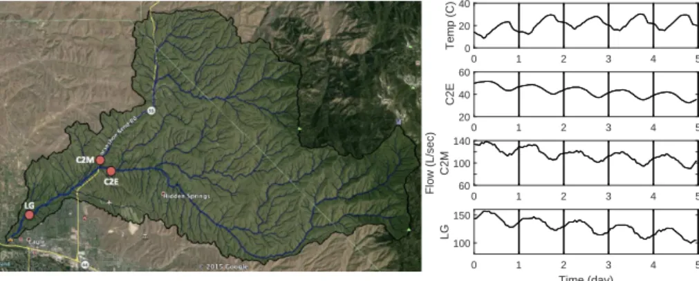
The Dry Creek Experimental Watershed in Idaho is a 28 km2 watershed where streamflow, soil moisture, and weather conditions are monitored at multiple locations ((McNa-mara, 2012)). At the outlet of the watershed (labeled Lower Gauge), diel signals can be seen in the streamflow dur-ing several of the years of observation durdur-ing which dry conditions occurred. We have focused our observations on the summer of 2011. The watershed includes seven stream gauging stations. One such station (Treeline) reported no streamflow for the duration of our observations. The report-ing gauges are named Bogus South (BS), Con1West (C1W), Con1East (C1E), Con2East (C2E), Con2Main (C2M), and Lower Gauge (LG). They drain upstream areas of 0.63, 3.85, 8.70, 7.54, 24.15, and 27.12, km2, respectively.
0 1 2 3 4 5
Temp (C) 0 20 40
0 1 2 3 4 5
C2E
20 40 60
0 1 2 3 4 5
Flow (L/sec)
C2M
60 100 140
Time (day)
0 1 2 3 4 5
LG
100 150
Figure 1.The left panel shows the Dry Creek watershed in Idaho. The right panel shows temperature (top), streamflow at gauge C2E near the center of the watershed (second), streamflow at gauge C2M (third), and streamflow at the outlet of the watershed (bottom). To demonstrate the delay in phases, a vertical line at the beginning of each day is included in each graph.
3 Developing an analytic solution for streamflow based on river network geometry
Let us now assume that the total subsurface runoff from each hillslope into a river link in a given river basin is oscillatory and its amplitude undergoes exponential decay (as seen for baseflow under dry conditions). Then, we define the runoff by the formula
R(t )=Be−A t+Ce−A tsin(2π ν(t−φ)), (1) withA,B,C, andν being positive parameters andC < B
to ensure that the baseflow takes only positive values. The phase shiftφrepresents an initial delay in observations due to water moving through the hillslope. In this paper, we apply the same baseflow pattern to all hillslopes on the river net-work beginning everywhere at an initial timet=0 (see the left panel of Fig. 2). Note that in this setup the runoff oscilla-tions are supposed to be driven by evapotranspiration, which is synchronized over all hillslopes at the catchment scale. For this reason, synchronized timing of the forcing seems an ac-ceptable hypothesis.
A sample baseflow pattern with parameter values A=
0.003 [h−1],B=0.08 [L s−1],C=0.008 [L s−1], andν=
1 24 [h−
1
] is illustrated in the right panel of Fig. 2. We chose the value ofν so that the frequency of the oscillations cor-responds to a period of 24 h, representing a diurnal signal. If we assume that the baseflow is linearly related to the amount of water in the soil, thenAcorresponds to the linear rate of water movement through the soil.
In this paper, the streamflow at the outlet of a river link is defined as the solution to the system of ordinary differential equations, which has been derived from the mass conserva-tion equaconserva-tion in the river links of the network, given by
dqi(t )
dt =K(qi)(R(t )+qi1(t )+qi2(t )−qi(t )). (2) The inputs to the link come from runoff on adjacent hill-slopes and from the streamflow of upstream tributary links.
1 2 3 4 5 6 7
0.05 0.06 0.07 0.08 0.09 0.10
Day
Flow
Figure 2.The left panel shows how runoff enters the river network as lateral flow from each hillslope to its adjacent link. The right panel shows a sample baseflow pattern given by Eq. (1) usingA= 0.003 [h−1],B=0.08 [L s−1],C=0.008 [L s−1],ν=241 [h−1], andφ=0[h].
Therefore, the only method for water to exit the watershed is as streamflow at the outlet link. In the equation,qi1andqi2 are the flows from the upstream tributary links. If a linkihas more than two tributaries at its upstream node, more terms can be added in Eq. (2), accordingly. For our calculation, we assume the functionK(qi)to be constant,K(qi)=vi/ l, whereviis the velocity of linkiandlis the length of the link, which is assumed to be uniform over all links in the network (Mantilla et al., 2011). For simplicity,K(qi)will be called
ki.
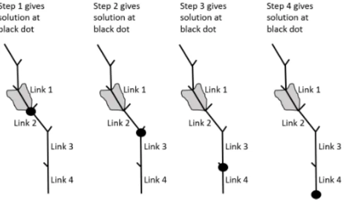
Figure 3.To determine the solution at any point, we consider runoff on only one hillslope (adjacent to link 1 in this case), and we trace the effects of that runoff downstream with no additional runoff from any subsequent hillslopes.
3.1 Propagation of hillslope runoff signal on river networks with uniform velocity
As mentioned above, we first apply runoffR(t )to a given hillslope, denoted as “hillslope a”, with adjacent river link 1. Because the transport equation for each link is linear, we can independently trace the runoff entering link 1 as it flows through the river network and then use superposition to com-bine the flows entering each river link. This would not be possible if the transport equation contained a nonlinear com-ponent. In the case of uniform velocities over the river net-work, the transport constant,ki, is subsequently the same for all links in the network. In this subsection, it will be calledk. When the runoff entering link 1 has gone throughoneriver link only (“step 1”; see Fig. 3), the flowq1at the outlet of link 1 is the solution to the differential equation
dq1(t )
dt =k(Be
−A t
+Ce−Atsin(2π ν(t−φ))−q1(t )). (3) That is,
q1=(q1(0)−J1+K1sin(2π ν(φ+θ ))e−kt+(J1
+K1sin(2π ν(t−φ−θ )))e−A t, (4) withq1(0)being the initial condition (att=0) of the flow in link 1 andK1,J1, andθdefined by
K1= Ck
p
(k−A)2+4π2ν2,
J1= Bk
k−A (5)
and
sin(2π νθ )=p 2π ν
(k−A)2+4π2ν2, cos(2π νθ )=p k−A
(k−A)2+4π2ν2. (6)
Note thatθ∈(0,4ν1)is the resulting time delay for the fluc-tuating patternq1(t )of frequency ν compared to the input signalR(t ).
At step 2, when the runoff has traversedtworiver links, we need to computeq2(t )by taking into account the solution
q1(t )from step 1 (see Fig. 3, second panel). Since we as-sumed for the moment thatq1(t )has been transmitted down-stream via the next link (link 2), with no additional runoff, the streamflow at the end of link 2 is given by
q2=(q2(0)−J2+K2sin(2π νθ2))
+kt (q1(0)−J1+K1sin(2π νθ1))e−kt
+ (J2+K2sin(2π ν(t−θ2)))e−A t, withθ1=φ+θ,θ2=φ+2θ, and
K2= Ck
2
(k−A)2+4π2ν2
J2= Bk
2
(k−A)2.
By mathematical induction, we then compute the solution
qn(t ), n≥1 of flow measured downstream at the exit from linkn. This takes the form
qn(t )=e−A t[Jn+Knsin(2π ν(t−θn))] +e−kt
n−1
X
j=0
Ln−j(kt ) j
j! (7) with coefficients
Kn=C
n
Y
j=1
k p
(k−A)2+4π2ν2
=C p k
(k−A)2+4π2ν2
!n
, n≥1
Jn=B
n
Y
j=1
k k−A=B
k
k−A n
, n≥1
θn=φ+ n
X
i=1
θ=nθ, n≥1 (8)
and
Lj=qj(0)−Jj+Kjsin(2π νθj) , j=1,2, . . .n. (9) Here,qj(0)represents the initial condition for the flow in linkj. For clarity, we included the details of this algorithmic proof in Appendix A.
3.2 Assembling the complete solution for streamflow at the outlet
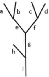
Figure 4.A small sample network to describe how total streamflow is computed.
over all links in the network (i.e., same parameterk) so that the influence of two links that are equidistant (topologically speaking) from the outlet will be the same. The solution de-termined in Sect. 3.1, however, shows only thepartial con-tributionof linkito the streamflow, as it propagates down-stream without considering any additional runoff. Therefore, in order to determine thecompletestreamflow solution, one must sum the overall contributions from runoff on each up-stream link. This can be done if the topological representa-tion of the river network is known or if the topological width function upstream of the outlet is used. The width function for a given linkiand distancen(denotedWn(i)) is an integer representing the number of river links of topological distance
nupstream of linki, whereW1(i)=1 and corresponds to link
i itself. For a fixed location in the river network, the width function can be written as a vector whose length is the diam-eter (i.e., the longest path) upstream of linki. The network depicted in Fig. 4 further illustrates this process.
First, we will focus on the outlet of link a (before the streamflow fromacombines with that of linkb); see Fig. 4. We recognize one link upstream of this point: linka. Then, the only contribution to the streamflow at this point is from the runoff to link a that has traversed one link. The width function at this point has only one element, and there is only one link of distance 1, so the width function, a one-dimensional vector, is given byW(a)= [1], and the stream-flow is simply
qa=1×q1=q1=L1e−kt+e−A t[J1+K1sin(2π ν(t−θ1))]. (10) On the other hand, if we compute streamflow at the outlet of linke(prior to joining linkf; see Fig. 4), we have one link of topological distance 1 (linke) and two links of topological distance 2 (linksa andb). Then, the width function is given by the vectorW(e)= [1 2]. This means that the runoff from linkehas only traversed one link to get to the outlet, but the runoff from either of the linksaorbhas traversed two links. The total flow at the outlet of linkeis
qe=1×q1+2×q2=q1+2q2. (11) After applying the formulas forq1andq2, similar terms can be collected in the following way:
qe=L1e−kt+e−A t[J1+K1sin(2π ν(t−θ1))]
+2
L2+ktL1
e−kt+2
J2+K2sin(2π ν(t−θ2))
e−A t
=e−A t(J1+2J2+K1sin(2π ν(t−θ1))
+2K2sin(2π ν(t−θ2)))+e−kt(L1+2[L2+ktL1]). (12) To complete this example, let us now consider the width function at the outlet of the network in Fig. 4, which is
W(i)= [1 2 2 4]. The first element ofW(i)corresponds to linki; the second element (W2(i)=2) corresponds to links
gandh; the third element (W3(i)=2) corresponds to links
eandf; and the last component (W4(i)=4) corresponds to linksa,b,c, andd. The diameter of this network isDi= length(W(i))=4. Note that the total number of links in the network is also the sum of the elements of the width function, since each link has a corresponding distance from the outlet. For this, we can use the notationW(i)
=PDni
=1W (i) n =9. For more details about the width function, see Mantilla et al. (2011) and Rodriguez-Iturbe and Rinaldo (2001). The flow at the outlet of linkiis
qi=1×q1+2×q2+2×q3+4×q4= Di X
n=1
Wn(i)qn. (13)
=e−A t(J1+2J2+2J3+4J4)+e−At(K1sin(2π ν(t−θ1))
+2K2sin(2π ν(t−θ2))+2K3sin(2π ν(t−θ3)
+ 4K4sin(2π ν(t−θ4)))+e−kt(L1+2[L2+ktL1]
+2
L3+ktL2+
(kt )2L1
2!
+ 4
L4+ktL3+
(kt )2L2
2! +
(kt )3L1
3!
. (14)
For a general network whose width function is given by
W(i), the solution can be rearranged as in Eqs. (12) and (14) to get the complete solution for streamflow at the outleti. Assuming thatDi is the diameter of the network upstream of linki, the solution at the outletiis
qi= e−A t Di X
n=1
Wn(i)[Jn+Knsin(2π ν(t−θn))]
+e−kt
Di X
n=1
Wn(i)
n−1
X
j=0
Ln−j(kt )
j
j! . (15)
The first term in Eq. (15) represents the propagation of the runoff signal from each hillslope, while the second term is a result of the initial conditions coming from runoff and flow in the network. This distinction is evidenced by the rate of de-cay of either exponential function. The first term has a rate of decay depending upon A and represents the decay of runoff entering the channel. The second term, conversely, has a de-cay rate dependent only uponk, which describes the rate of water movement through each river link.
and use the expected parameter values to discuss the mathe-matical solution. First,kandAare both positive because they represent rates of water movement along the river link and through the soil, respectively. Since water will move much more quickly along the river link, which offers less resis-tance than soil, A is significantly less thank, so that k−kA has a value slightly greater than 1. Then, Jj> B for any value ofj. Furthermore, the value of 2π νis fixed and is typ-ically greater thank, which means that √ k
(k−A)2+4π2ν2 <1, so thatKj < C for all j. This means that each component
[Jn+Knsin(2π ν(t−θn))]of the solution at the outlet shows a decrease in the amplitude of the fluctuations (Kn < C) while increasing its average value when compared with the runoff function (Jn > B).
In the limiting case ofA=0, the runoff at each hillslope would be a sinusoidal wave of amplitudeCand average value
B taking the formR=B+Csin(2π νt ). Then, the solution at the outlet becomes
qi= Di X
n=1
Wn(i)[Jn+Knsin(2π ν(t−θn))]
+ e−kt
Di X
n=1
Wn(i)
n−1
X
j=0
Ln−j(kt )
j
j! , (16)
whereKn,Jn, andθare defined byKn=CQn i=1√ k
k2+4π2ν2,
Jn=B, and sin(2π νθ )=√ 2π ν
k2+2π2ν2 and cos(2π νθ )= k
√
k2+2π2ν2.
It is apparent that the second sum of Eq. (16) that includes exponential decay at the rate of water movement through the river link is the transient term. The first sum of Eq. (16) is the asymptotic solution and includes the sum of constant terms from each hillslope and the sum of amplitudes of the sine waves from each hillslope. Following a similar approach in the case of A >0 and using the fact thatA≪k, we again find that the second term in Eq. (15) decays much faster; consequently,e−A tPDi
n=1W (i)
n [Jn+Knsin(2π ν(t−θn))]can be interpreted as being the asymptotic solution of qi. Due to interference from sinusoidal waves that can be in or out of phase, the amplitude of the asymptotic solution inqi can change depending on the phase shift. We investigate this de-pendence in Sect. 4.
4 Results
4.1 Testing design: examining the effects of velocity on streamflow amplitude and time delay downstream In order to test the competing hypotheses by Wondzell et al. (2007) and those presented in Graham et al. (2013), we will demonstrate the amplification and damping of the oscillatory streamflow signal that are caused by superposition. We con-sider a sample network and compute the streamflow solution
at different locations in the river network when the velocity and its corresponding time delay are varied. We will consider both the uniform (withvi=vfor all linksi) and the variable velocity cases.
We compute the streamflow solution for the Mandelbrot– Vicsek tree of magnitude 14, as shown in Fig. 5. The Mandelbrot–Vicsek tree is self-similar (Mandelbrot and Vic-sek, 1989) and has been used to demonstrate hydrologic properties at different scales (e.g., Mantilla et al., 2006; Peck-ham, 1995). In this figure, the label next to each link repre-sents the magnitude of the link, which describes the scale of the link and is determined by the sum of the magnitudes of the two immediate upstream “parent” links where exter-nal links have magnitude 1. The constant parameter values used in this example are A=1.2×10⁻⁴ [h−1], B=0.08 [L s−1],C
=0.008 [L sec−1],q
0=0.08 [L sec−1], andν= 1
24 [h−
1] and are uniform over each link in the network. To test the effects of superposition on streamflow, we will sim-ulate streamflow for different transport constantsk. Figure 6 shows the simulation runoff pattern (top) along with the sam-ple streamflow solution at the outlet of the network in the uniform case (bottom). To distinguish among the different simulations, we will narrow our view to a few oscillations, which are highlighted by a box in the panels in Fig. 6. 4.2 Uniform velocity over the river network
In the case of uniform velocities, the streamflow at the out-let is given by the solution to Eq. (15). The time delay de-pends upon parameters that have physically based values (see Eq. 6), so a realistic range for the time delay and phase shift can be found. These parameters,k andA, are incorporated in other parts of the solution (see Eq. 8). Therefore, chang-ing their values impacts the solution in more ways than just the superposition of sinusoidal functions. The physical value represented byAis expected to remain constant for a given region. On the other hand,krepresents the inverse of the res-idence time in each river link and is not necessarily uniform or fixed.
Recall thatkis given by vl, wherevis the stream velocity andlis the stream length. The length of each river link in a real river network would be different, as would the velocity. In addition, the velocity may change over time, since velocity increases with flow. Consequently, the realistic value ofkis expected to be different for each link in the network, and the uncertainty ofkis a possible source for different time delays and phase shifts.
Figure 5.The Mandelbrot–Vicsek tree of magnitude 14. The nitude of each link is written next to the link. One link of each mag-nitude is distinguished by the dots along the network.
0 50 100 150 200 0.065
0.07 0.075 0.08 0.085 0.09
Time (h)
Runoff (liter/sec)
0 50 100 150 200
1.8 1.9 2 2.1 2.2 2.3 2.4 2.5
Time (h)
Flow (liter/sec)
Figure 6.Sample runoff pattern (top) and resulting streamflow so-lution at the outlet in the uniform case (bottom) fork=vl To ex-amine the oscillations more closely for different velocities, we will focus on a small section of the solution (highlighted by a box in each panel).
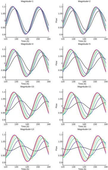
The results of simulating streamflow in the Mandelbrot– Viscek tree using different values ofkcan be found in Fig. 7. The values ofkused in simulations are 0.38, 0.7, 1.02, 1.34, 1.66, 1.98, and 2.30 with resultant time delays of 2.30, 1.36, 0.95, 0.73, 0.59, 0.5, and 0.43 h. The corresponding graph so-lutions from Fig. 7 are drawn in the following colors: black, blue, green, cyan, orange, red, and purple, respectively. Each panel in Fig. 7 represents the solution at a different loca-tion along the network (refer to Fig. 5 for sample localoca-tions).
120 130 140 150 160
0.9 0.95 1 1.05 1.1
Time (h)
Flow
Magnitude=1
120 130 140 150 160
0.9 0.95 1 1.05 1.1
Time (h)
Flow
Magnitude=2
120 130 140 150 160
0.9 0.95 1 1.05 1.1
Time (h)
Flow
Magnitude=4
120 130 140 150 160
0.9 0.95 1 1.05 1.1
Time (h)
Flow
Magnitude=5
120 130 140 150 160
0.9 0.95 1 1.05 1.1
Time (h)
Flow
Magnitude=10
120 130 140 150 160
0.9 0.95 1 1.05 1.1
Time (h)
Flow
Magnitude=11
120 130 140 150 160
0.9 0.95 1 1.05 1.1
Time (h)
Flow
Magnitude=13
120 130 140 150 160
0.9 0.95 1 1.05 1.1
Time (h)
Flow
Magnitude=14
Figure 7.Flows at the outlet of each magnitude link using different k in each river simulation. The k values (with units of h−1) are 0.38, 0.7, 1.02, 1.34, 1.66, 1.98, and 2.30 and are colored black, blue, green, cyan, orange, red, and purple, respectively. The flows are normalized about the average flow.
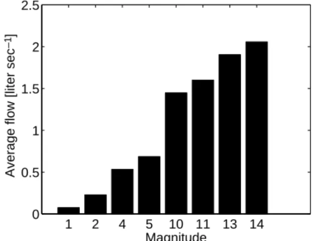
veloc-1 2 4 5 10 11 13 14 0
0.5 1 1.5 2 2.5
Magnitude
Average flow [liter sec ]
–1
Figure 8. Average flows at different locations along the Mandelbrot–Vicsek tree.
ity is highest, which moves a volume of water very quickly through each link and leads to very little loss of streamflow intensity. Notice also that the timing of the peak stream-flow is increasingly delayed as velocity slows (see Fig. 7 for
k=0.38, 1.02, and 1.66, for example). This can explain the increasing time delay that has been observed between maxi-mum evapotranspiration and minimaxi-mum streamflow as the dry season progresses. These results also indicate that the time delay increases continuously as the velocity decreases con-tinuously over time so that the time delay can be predictable depending upon stream velocity.
At the link of magnitude 1, the phase shift has little influ-ence on the amplitude and only has an influinflu-ence on the timing of the wave. At the outlet of a magnitude-2 link, the two up-stream links are “in phase”, meaning they have the same time delay as each other since they are the same topological dis-tance from the point at which we compute streamflow. There-fore, these two will exhibit constructive interference. When they are combined with the downstream link, however, the different values of phase shift can result in constructive or destructive interference, although they never completely de-stroy the oscillations. The phase shift that produces the max-imum streamflow is zero because this represents the face that all three streamflows that feed into this outlet are completely in phase.
As we examine the streamflows in links with greater mag-nitude, the shape of the network (described by the width function) becomes important because the flows from all links of a given distance will reach the outlet at the same time. Be-ing out of phase with links of other distances can cause some reduction in the amplitude of the streamflow oscillations, but the oscillations will not be completely destroyed.
4.3 Propagation of oscillations on a real network In this section, we apply the analytic streamflow solution for uniform conditions to the river network of the Dry Creek
river basin to study the effects of scale on streamflow ampli-tude and timing. In the previous section, we also examined the flow at different scales (see Fig. 7) but with an emphasis on differentkvalues. The time range in Fig. 7 has been de-creased, and the flows have been normalized about their av-erage value to exaggerate the effects of changing thekvalue. Consider the blue line in all panels of Fig. 7 corresponding to ak value of 0.7 h−1. Streamflow at a larger scale (mag-nitude) is influenced by a greater number of upstream links. Hence, superposition effects among those upstream links are stronger, and we see two resulting attributes in the stream-flow properties: reduction in the streamstream-flow amplitude and greater time delay to the peak. We now consider a larger, more realistic river network and expect to see similar results. In our theoretical examples, we assumed the length of each link to be uniform over the river network, so that changes in velocity directly correspond to changes in the transport con-stant k. Realistic network parameters include variable link length, so we vary the velocity of each link accordingly in order to maintain a uniformk value and apply the solution developed in Sect. 3.
For a comparison with available data, we revisit informa-tion from the Dry Creek Experimental Watershed in Idaho. Using streamflow data from LG, the gauge nearest the wa-tershed outlet along with topological data retrieved using the program CUENCAS proposed in (Mantilla and Gupta, 2005), we can compare the diel flows observed in 2011 with the solution method used in Sect. 3. Specifically, the solution to describe streamflow at the outlet, given in Eq. (16), can be fitted to the observed streamflow to find parameter val-ues A, B, and C that uniquely describe baseflow exiting each hillslope. The assumption inherent in this solution is that the river links are all uniform, which is an unrealistic but neces-sary simplification to develop this explicit solution. The top left panel of Fig. 9 depicts the observed streamflow from July of 2011 along with our approximated solution that was found by fitting the data to Eq. (16) using MATLAB. The resulting parameter values are
A=1.85×10⁻³ [h−1]
B=0.239 [L s−1]
C=3.27×10⁻² [L s−1]
φ=3.97 [h]
k=5.61 [h−1].
For perspective, this k value corresponds to an average stream velocity of 0.38 m s−1.
Using the observed streamflow time series at several up-stream gauges in the Dry Creek watershed, we can test our analytic solution with the parameters determined above. If we treat these locations as the outlets of smaller embedded watersheds, we can again apply Eq. (16) using the same pa-rameter values which will yield our solution at pointsalong
[t]
Time [h]
0 100 200 300 400
60 80 100 120 140
160 Lower Gauge
Observed Computed
Time [h]
0 100 200 300 400
50 100
150 Gauge C2M
Observed Computed
Time [h]
0 100 200 300 400
Flow [L sec ]
10 20 30 40 50
60 Gauge C2E
Observed Computed
–1
Flow [L sec ]
–1
Flow [L sec ]
–1
Figure 9.Observed streamflow and streamflow fitted using Eq. (16) at the outlet of the Dry Creek Experimental Watershed (top) and at two stream gauges upstream in the watershed: Con2Main (center) and Con2East (bottom).
Although the predicted streamflow given by our solution does not fit the data as well for C2E as it does for C2M, we can see that the magnitude of our predicted streamflow is very close to observed streamflow at either location. Fur-thermore, the timing of the oscillations is nearly identical for both C2M and C2E. In the presence of heterogeneity on the hillslope and along the river network, we must be flexible about the amount of data we can reasonably expect to fit well.
For example, we show in Appendix B that the data are more noisy at other gauges in the Dry Creek watershed where we compare observed streamflow data to our streamflow solu-tion.
Because our solution fits the data reasonably well at sev-eral locations along the river network where runoff is uni-formly enforced, we can be assured of the internal validity of using a solution such as that given in Eq. (16). Further-more, because our solution describes superposition among all the oscillating runoff signals entering the network, and the simulation results are close to those observed, we can con-clude that streamflow relies heavily on superposition from upstream in the river network as suggested in (Wondzell et al., 2007).
5 Conclusions and future work
Observations of oscillatory streamflow during low-flow con-ditions have highlighted the magnitude and time delay caused by the diel signal that represents evapotranspiration. Several current hypotheses suggest that the properties of the oscillatory streamflow signal can be attributed to differ-ent methods of water movemdiffer-ent through the subsurface, al-though another hypothesis suggests that flow along the river determines the timing and amplitude of oscillations. In this paper, we provide evidence to support the latter argument.
First, we select a mathematical function according to streamflow observations at the catchment scale to represent baseflow patterns at the hillslope scale. The selected baseflow pattern is applied as input to a linear transport equation for all links in a river network that are assumed to have uniform properties and parameter values. For this uniform situation, we develop an analytic solution to represent streamflow at any point in a river network. We compute the solution by sep-arately determining the partial streamflow at the outlet from each river link and then taking the sum over all river links in the river network. In order to include the geomorphology of the river network, we use the width function to compute the complete streamflow solution. We have also extended the streamflow solution to include nonuniform links in the river network.
supports the hypothesis of Wondzell et al. (2007). Further-more, the structure of the analytic solution indicates that the time delay increases continuously as the river network ve-locity continuously decreases, so that the time delay can be predictable depending on stream velocity. We apply the re-sulting solution to several locations in the Dry Creek Exper-imental Watershed using parameters determined by stream-flow at the outlet. We then compare the streamstream-flows result-ing from our solution with observations. Our solution offers a good approximation for the streamflow at locations with larger upstream area (e.g., LG, C2M, and C2E), matching the magnitude of the streamflow and the amplitude and tim-ing of the oscillations. Our results, however, do not disprove the hypothesis that delays can come from subsurface flow processes.
As a next step, we propose to test the analytic solutions herein in networks with different geomorphological struc-tures in order to compare the resulting streamflow ampli-tudes and emphasize the dependence upon network geom-etry. We suggest subsequently comparing our analytic so-lutions with the numerical results obtained using nonlinear transport equations, which will demonstrate the relationship between link propagation at the hillslope scale and stream-flow at the catchment scale. Careful field experiments would be necessary to provide a definitive conclusion about the at-tribution of time delays.
6 Data availability
Appendix A: Development of streamflow solution for uniformkvalue over all links in the river network In order to simplify our calculations below, we will use the notationω=2π νandψ=2π νφ.
We prove Eq. 7 from Sect. 3.1 by using the method of mathematical induction. The isolated effects of runoff from linkion links downstream are found by applying the trans-port equation
dqi(t )
dt =k(Be
−A t
+Ce−A tsin(ωt−ψ )−qi(t )). (A1) We did not include in Eq. (A1) any upstream links because we are trying to isolate the effects on streamflow due to runoff from hillslope i. Therefore, we treat it as an exter-nal link. Equation (A1) is a nonhomogeneous linear ordinary differential equation of the form
dqi
dt =kfi(t )−kqi, (A2)
and has the solution
qi(t )=qi(0)e−kt+ke−kt t
Z
0
fi(s)eksds. (A3)
As we trace the runoff downstream, the functionfi(t )is the input to the link, which can come from upstream sources or from runoff from the adjacent hillslope. Since link i is ar-bitrary, we will consider it to be the first link in a path to the outlet, so it will be labeled link 1, having flowq1, and the next link downstream will be labeled link 2, etc. Since
f1(t )consists only of baseflow, the solutionq1according to Eq. (A3) becomes
q1(t )= q1(0)e−kt+ke−kt t
Z
0
h
Be(k−A)s
+Ce(k−A)ssin(ωs−ψ )ids
= q1(0)e−kt+Bke−kt
e(k−A)t k−A −
1
k−A !
+Cke−kt
t
Z
0
e(k−A)ssin(ωs−ψ )ds. (A4)
The solution to the latter integral is
t
Z
0
e(k−A)ssin(ωs−ψ )ds= e
(k−A)t
p
(k−A)2+ω2sin(ωt−ψ−ϕ)
+psin(ψ+ϕ) (k−A)2+ω2,
andϕis defined by its sine and cosine functions: sin(ϕ)=p ω
(k−A)2+ω2,
cos(ϕ)=p k−A (k−A)2+ω2.
Substituting this integral back into Eq. (A4), we obtain
q1(t )= q1(0)− k k−AB+
k p
(k−A)2+ω2Csin(ψ+ϕ) !
e−kt
+ k
k−AB+ k p
(k−A)2+ω2Csin(ωt−ψ−ϕ) !
e−A t. (A5) To find an algorithmic method to compute the coefficients of the solutionqn(t )forn≥1, we define the following:
Kn=C
n
Y
j=1
k p
(k−A)2+ω2 n≥1, (A6)
Jn=B
n
Y
j=1
k
k−A n≥1, (A7)
8n=ψ+ n
X
j=1
ϕ n≥1, (A8)
Lj=qj(0)−Jj+Kjsin(8j) j=1, . . ., n. (A9) Using these newly defined quantities from Eqs. (A6), (A7), (A8), and (A9), the flow at the outlet of link 1 can be rewritten as
q1=L1e−kt+e−A t[J1+K1sin(ωt−81)]. (A10) To find the solution for the next link downstream (link 2), the flow from link 1, given by Eq. (A10), is included asqin1 as the transport Eq. (2) is applied to link 2. Integration by parts will again be used to find the solution to
dq2
dt =k(q1−q2).
Using Eq. (A3),
q2(t )= q2(0)e−kt+ke−kt t
Z
0
q1(s)eksds
= q2(0)e−kt+ke−ktL1t+ke−ktJ1 e(k−A)t
k−A − 1 k−A
!
+ ke−ktK1 t
Z
0
e(k−A)ssin(ωs−81)ds. (A11)
The integral in Eq. (A11) is very similar to that in Eq. (A4), with the only differences being the argument of the sine func-tion in the initial integral. After integrafunc-tion by parts, the equa-tion for streamflowq2(t )becomes
q2= q2(0)e−kt+ke−ktL1t+ke−ktJ1
e(k−A)t k−A −
1
+ke−ktK1 1 p
(k−A)2+ω2
e(k−A)tsin(ωt−82)+sin(82)
!
or, equivalently,
q2=L2+ktL1e−kt+J2+K2sin(ωt−82)e−A t. (A12)
By mathematical induction, using the same strategy for cal-culations along the path to the river network outlet, we can compute the contribution of runoff from any river link to flow at the outlet. For a given link that is at topological distancen
from the outlet (or an alternative location from which flow is observed), its contribution to the flow at the outlet is
qn(t )=e−A t[Jn+Knsin(ωt−8n)]+e−kt n−1
X
j=0
Ln−j(kt )
j
j! .
(A13) Given that ω=2π ν and using the notation ϕ=2π νθ, Eqs. (6), (7), (8), and (9) immediately will result.
Time [h]
0 100 200 300 400
20 30 40 50 60
70 Gauge C1E
Observed Computed
Time [h]
0 100 200 300 400
5 10 15 20 25
30 Gauge C1W
Observed Computed
Time [h]
0 100 200 300 400
Flow [L sec ]
0 5 10 15 20 25 30
35 Gauge Bogus South Observed Computed
–1
Flow [L sec ]
–1
Flow [L sec ]
–1
Figure B1. Observed streamflow and streamflow fitted using Eq. (16) at three upstream gauges in the Dry Creek Experimental Watershed: Con1East (top), Con1West (center), and Bogus South (bottom).
respectively) – recorded streamflows which can be found in Fig. B1 along with our solution given by Eq. (16) at those locations.
As can be seen in Fig. B1, our solution does not offer a good fit to observed data at these three locations. Both C1E and Bogus supply noisy signals, which do not have the obvious daily oscillations characteristic of the streamflows further downstream. The magnitude of the observed stream-flow at Bogus is particularly interesting, because the area up-stream of the gauge is 0.634 km2, and the average streamflow is around 18 L s−1. The streamflow at C1W is similar, with a magnitude of the average streamflow of about 13 L s−1, but the area upstream of C1W is 3.85 km2, so we should expect a significant difference between the streamflows at these two locations, and C1W should certainly experience larger values than Bogus. Because of this, we believe the observed stream-flow at the Bogus site is unreliable.
The observed and predicted streamflow at the location C1E can be found in the left panel of Fig. B1. Again, the observations are especially noisy and have no apparent daily oscillations. However, our solution for streamflow has mag-nitude very close to observed values. We cannot conclude from this that our solution is incorrect, but it relied upon the assumption of smooth oscillatory runoff even at the hillslope scale. These noisy signals imply that the assumption is incor-rect at some locations.
Acknowledgements. This material is based on work supported by the National Science Foundation under grant number NSF DMS-1025483 and financial support from the Iowa Flood Center. The authors also want to acknowledge Witold Krajewski from the University of Iowa and IIHR for helpful discussions and feedback during the preparation of the manuscript.
Edited by: T. Hengl
References
Arnell, N.: The effect of climate change on hydrological regimes in Europe: a continental perspective, Global Environ. Chang. 9 5–23, 1998.
Bond, B., Jones, J., Moore, G., Phillips, N., Post, D., and McDon-nell, J.: The zone of vegetation influence on baseflow revealed by diel patterns of streamflow and vegetation water use in a headwa-ter basin, Hydrol. Process., 16, 1671–1677, 2002.
Burn, D., Buttle, J., Caissie, D., MacCulloch, G., Spence, C., and Stahl, K.: The Processes, Patterns and Impacts of Low Flows Across Canada, Canad. Water Resour. J., 33 107–124, 2008. Burt, T. P.: Diurnal variations in stream discharge and throughflow
during a period of low flow, J. Hydrol., 41 291–301, 1979. Graham, C., Barnard, H., Kavanagh, K., and McNamara, J.:
Catch-ment scale controls the temporal connection of transpiration and diel fluctuations in streamflow, Hydrol. Process., 27 2541–2556, 2013.
Gribovszki, Z., Kalicz, P., Szilagyi, J., and Kucsara, M.: Ripar-ian zone evapotranspiration estimation from diurnal groundwater level fluctuations, J. Hydrol., 349 6–17, 2008.
Gribovszki, Z., Szilagyi, J., and Kalicz, P. Diurnal fluctuations in shallow groundwater levels and streamflow rates and their inter-pretation – A review, J. Hydrol., 385, 371–383, 2010.
McNamara, J. and Aishlin, P.: Dry Creek Data, https://earth. boisestate.edu/drycreek/data/, 2016.
Mandelbrot, B. B. and Vicsek, T. Directed recursive models for frac-tal growth, J. Phys., 22, L377–L383, 1989.
Mantilla, R. and Gupta, V. K.: A GIS numerical framework to study the process basis of scaling statistics in river networks, Geosci. Remote Sens. Lett., 2.4 404–408, 2005.
Mantilla, R., Gupta, V., and Mesa, O.: Role of coupled flow dy-namics and real network structures on Hortonian scaling of peak flows, J. Hydrol., 322, 155–167, 2006.
Mantilla, R., Gupta, V. K., and Troutman, B. M.: Scaling of peak flows with constant flow velocity in random self-similar networks, Nonlin. Processes Geophys., 18, 489–502, doi:10.5194/npg-18-489-2011, 2011.
McNamara, J. P.: Continuous monitoring in the Dry Creek Ex-perimental WatershedHydrologic Sciences, Dept of Geoscience, Boise State University, Boise, ID, 2012.
Mul, M., Kemerink, J., Vyagusa, N., Mshana, M., van der Zaag, P., and Makurira, H.: Water allocation practices among small-holder farmers in the South Pare Mountains, Tanzania: The issue of scale, Agr. Water Manage., 98, 1752–1760, 2011.
Peckham, S.: New results for self-similar trees with applications to river networks, Water Resour. Res., 31, 1023–1029, 1995. Rodriguez-Iturbe, I. and Rinaldo, A. Fractal river basins: chance
and self-organization Cambridge University Press, 15–18, 2001. Stott, R. E. and Burt, T. P.: Potassium chemistry of a small upland stream following a major drought, Hydrol. Process., 11, 189– 201, 1997.
Wondzell, S., Gooseff, M., and McGlynn, B.: Flow velocity and the hydrologic behavior of streams during baseflow, Geophys. Res. Lett., 34, L24404, doi:10.1029/2007GL031256, 2007.