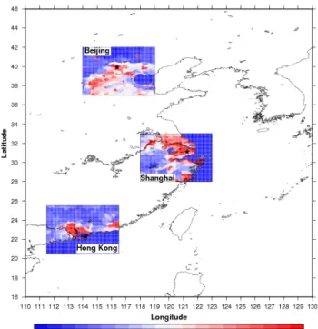
IASI observations of seasonal and day-to-day variations of tropospheric ozone over three highly populated areas of China: Beijing, Shanghai, and Hong Kong

Abstract: This paper proposes a systematic method for the simultaneous determination of adjusted ranks of sample observations and their sums and products adjusted for

Foram produzidos queijos do “Marajó” tipo creme em dois locais (Local A - Universidade do Estado do Pará e Local B - Laticínios de Soure, Ilha do Marajó, Pará)..

The rise of Hong Kong coincided exactly with the fall of Shanghai, but the re-rise of Shanghai need not to spell the demise of Hong Kong whose growth rests on China’s

Features of the retrieved methane space-time distribution include: (1) a strong sea- sonal cycle of 30 ppbv in the northern tropics with a maxi- mum in January–March and a minimum

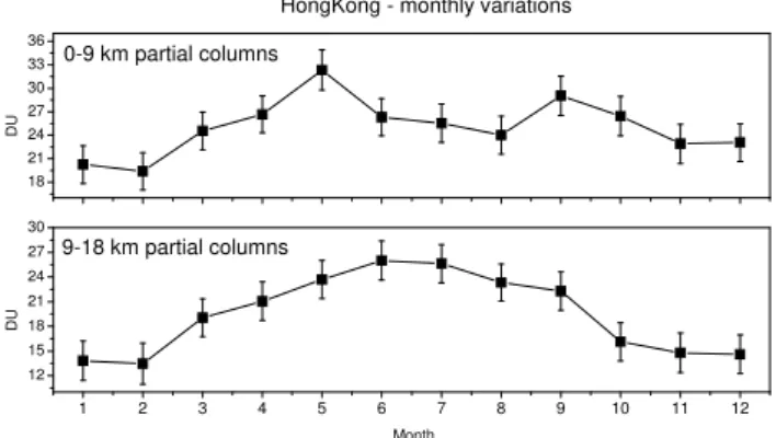
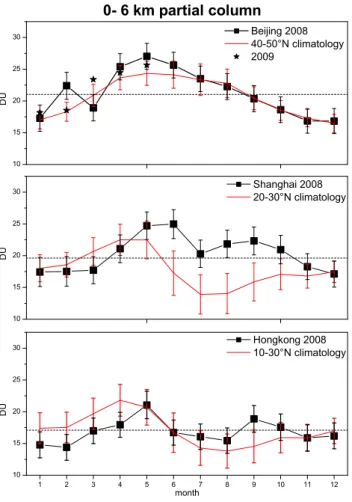
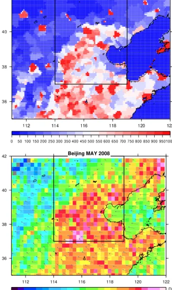
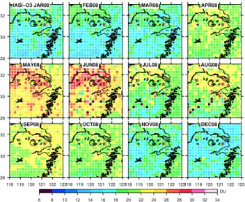
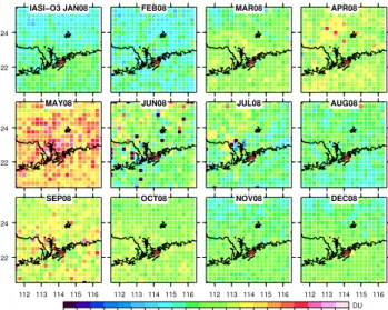
The monthly mean variations of lower tropospheric ozone mea- sured with IASI (partial columns and profiles) show the influence of the summer Asian monsoon on the ozone

2 Hong Kong Institute of Diabetes and Obesity, The Chinese University of Hong Kong, Hong Kong SAR, People’s Republic of China, 3 Li Ka Shing Institute of Health Science, The

The probability of attending school four our group of interest in this region increased by 6.5 percentage points after the expansion of the Bolsa Família program in 2007 and

On average for all the years in the time series below, the IASI limits of confidence are 1.9, 1.7, and 1.5 ppb for the Eastern Asia, Western US, and Europe ROI, respectively.. In