Combined assimilation of IASI and MLS observations to constrain tropospheric and stratospheric ozone in a global chemical transport model

(1)

ACPD

13, 21455–21505, 2013

Combined assimilation of IASI

and MLS ozone observations

E. Emili et al.

Title Page

Abstract Introduction

Conclusions References

Tables Figures

◭ ◮

Back Close

Full Screen / Esc

Printer-friendly Version Interactive Discussion

Discussion

P

a

per

|

D

iscussion

P

a

per

|

Discussion

P

a

per

|

Discuss

ion

P

a

per

Atmos. Chem. Phys. Discuss., 13, 21455–21505, 2013 www.atmos-chem-phys-discuss.net/13/21455/2013/ doi:10.5194/acpd-13-21455-2013

Atmospheric Chemistry and Physics

Open Access

Discussions

Geoscientiic Geoscientiic

This discussion paper is/has been under review for the journal Atmospheric Chemistry and Physics (ACP). Please refer to the corresponding final paper in ACP if available.

Combined assimilation of IASI and MLS

observations to constrain tropospheric

and stratospheric ozone in a global

chemical transport model

E. Emili1, B. Barret3, S. Massart4, E. Le Flochmoen3, A. Piacentini1, L. El Amraoui2, O. Pannekoucke1,2, and D. Cariolle1

1

CERFACS, Toulouse, France

2

Météo France, Toulouse, France

3

Laboratoire d’Aérologie, Toulouse, France

4

ECMWF, Reading, UK

Received: 15 July 2013 – Accepted: 30 July 2013 – Published: 20 August 2013

Correspondence to: E. Emili (emili@cerfacs.fr)

(2)

ACPD

13, 21455–21505, 2013

E. Emili et al.

Title Page

Tables Figures

◭ ◮

Back Close

Full Screen / Esc

Discussion

P

a

per

|

D

iscussion

P

a

per

|

Discussion

P

a

per

|

Discuss

ion

P

a

per

|

Abstract

Accurate and temporally resolved fields of free-troposphere ozone are of major im-portance to quantify the intercontinental transport of pollution and the ozone radiative forcing. In this study we examine the impact of assimilating ozone observations from the Microwave Limb Sounder (MLS) and the Infrared Atmospheric Sounding

Interfer-5

ometer (IASI) in a global chemical transport model (MOdèle de Chimie Atmosphérique à Grande Échelle, MOCAGE). The assimilation of the two instruments is performed by means of a variational algorithm (4-D-VAR) and allows to constrain stratospheric and tropospheric ozone simultaneously. The analysis is first computed for the months of August and November 2008 and validated against ozone-sondes measurements

10

to verify the presence of observations and model biases. It is found that the IASI Tropospheric Ozone Column (TOC, 1000–225 hPa) should be bias-corrected prior to assimilation and MLS lowermost level (215 hPa) excluded from the analysis. Further-more, a longer analysis of 6 months (July–August 2008) showed that the combined assimilation of MLS and IASI is able to globally reduce the uncertainty (Root Mean

15

Square Error, RMSE) of the modeled ozone columns from 30 % to 15 % in the Upper-Troposphere/Lower-Stratosphere (UTLS, 70–225 hPa) and from 25 % to 20 % in the free troposphere. The positive effect of assimilating IASI tropospheric observations is very significant at low latitudes (30◦S–30◦N), whereas it is not demonstrated at higher latitudes. Results are confirmed by a comparison with additional ozone datasets like

20

the Measurements of OZone and wAter vapour by aIrbus in-service airCraft (MOZAIC) data, the Ozone Monitoring Instrument (OMI) total ozone columns and several high-altitude surface measurements. Finally, the analysis is found to be little sensitive to the assimilation parameters and the model chemical scheme, due to the high frequency of satellite observations compared to the average life-time of

free-troposphere/low-25

(3)

ACPD

13, 21455–21505, 2013

E. Emili et al.

Title Page

Tables Figures

◭ ◮

Back Close

Full Screen / Esc

Discussion

P

a

per

|

D

iscussion

P

a

per

|

Discussion

P

a

per

|

Discuss

ion

P

a

per

1 Introduction

Tropospheric ozone (O₃) is the third most important gas in its contribution to the global greenhouse effect after CO₂and CH₄(Solomon et al., 2007). It is also a major pollutant in the planetary boundary layer, with adverse e_ffects on humans health (Brunekreef and Holgate, 2002) and plants (Avnery et al., 2011). Its production is mainly driven

5

by emissions of primary pollutants such as nitrogen oxides (NO_x), carbon monoxide (CO) and Volatile Organic Compounds (VOCs), followed by photolysis and non-linear chemistry reactions. Since it has an average life-time of about two weeks, it can be ef-ficiently transported for several thousands of km in the free troposphere (Zhang et al., 2008; Ambrose et al., 2011). Quantifying the impact of tropospheric ozone transport

10

is especially important for those countries that, despite air-quality related regulations, experience a significant ozone background increase (Jaffe and Ray, 2007; Tanimoto, 2009). Moreover, intrusions of ozone-rich air from the stratosphere via stratosphere-troposphere exchanges (STE) are among the principal causes of high free-stratosphere-troposphere ozone episodes (Stohl et al., 2003; Barré et al., 2012). Therefore, a precise

characteri-15

zation of both low-stratosphere and tropospheric ozone is required to properly quantify ozone transport.

Ozone-sondes provide observations of tropospheric and stratospheric ozone with high vertical resolution (Komhyr et al., 1995), but their geographical distribution is sparse and they are not very frequent in time. Satellite observations of ozone are

avail-20

able since the early 70s (Fioletov et al., 2002) but they provided mainly stratospheric ozone profiles or total columns. Since the stratospheric ozone concentration is higher than the tropospheric one by several orders of magnitude, total column retrievals do not provide a strong sensitivity to tropospheric ozone. Several studies derived tropospheric ozone columns by means of subtracting the measured stratospheric amount from the

25

(4)

ACPD

13, 21455–21505, 2013

E. Emili et al.

Title Page

Tables Figures

◭ ◮

Back Close

Full Screen / Esc

Discussion

P

a

per

|

D

iscussion

P

a

per

|

Discussion

P

a

per

|

Discuss

ion

P

a

per

|

The latest generation of thermal infrared spectrometers, onboard low-earth orbit (LEO) satellites, is able to capture the tropospheric ozone signature (Eremenko et al., 2008; Boynard et al., 2009; Barret et al., 2011; Tang and Prather, 2012). The Tropospheric Emission Spectrometer (TES) provides for example almost two pieces of independent information (degrees of freedom for signal, DFS) in the troposphere (Zhang et al., 2010)

5

with a global coverage in 16 days. The Infrared Atmospheric Sounding Interferometer (IASI) allows a daily global coverage at very high spatial resolution (12 km for nadir observations), with a slightly reduced number of tropospheric DFS (_∼1, Dufour et al., 2012), although the DFS value might also be sensible to the choice of the tropopause height and the retrieval technique. In general, satellites data permit to catch major

10

features of ozone tropospheric distribution (Ziemke et al., 2009; Hegarty et al., 2010; Barret et al., 2011) but observations frequency and data gaps (e.g. due to clouds) do not allow a complete view of the underlying dynamics at short time scales (e.g. hours). Chemical transport models (CTM), through data assimilation (DA), can ingest infor-mation from satellite observations in a coherent way (e.g. by considering the vertical

15

sensitivity of the instrument) and use them to update the modeled 3-D ozone field. Likewise, satellite retrievals themselves are normally based on the inversion of the measured radiance data with a variational approach, thus requiring an a-priori profile from a model or a climatology as ancillary input (Eskes and Boersma, 2003). Data as-similation of stratospheric ozone profiles, total columns or ozone sensitive radiances

20

is nowadays well integrated in operational meteorological models (Jackson, 2007; Dee et al., 2011), which are generally based on simplified ozone chemistry schemes (Geer et al., 2007). Assimilation of satellite O₃products has also been investigated in a num-ber of studies with CTMs including comprehensive chemistry schemes (Geer et al., 2006; Lahoz et al., 2007b; van der A et al., 2010; Doughty et al., 2011). Furthermore,

25

(5)

ACPD

13, 21455–21505, 2013

E. Emili et al.

Title Page

Tables Figures

◭ ◮

Back Close

Full Screen / Esc

Discussion

P

a

per

|

D

iscussion

P

a

per

|

Discussion

P

a

per

|

Discuss

ion

P

a

per

Parrington et al. (2009) and Miyazaki et al. (2012) assimilated TES data to constrain tropospheric ozone, finding consistent improvements with regard to the respective model background field. However, few studies explored the assimilation of ozone data from IASI, which is the only sensor sensible to tropospheric ozone and with a global daily coverage (night and day). Massart et al. (2009) assimilated IASI total columns but

5

did not use averaging kernel informations to separate tropospheric and stratospheric signal. Han and McNally (2010) assimilated IASI radiances in the ECMWF 4-D-VAR system and found a better fit of the analysis to ozone profiles from the Microwave Limb Sounder (MLS), but effects on tropospheric ozone were not discussed. Coman et al. (2012) assimilated 0–6 km ozone columns in a regional CTM and found improved

10

ozone concentrations also at the surface. To our knowledge there is still no study that examined the assimilation of IASI tropospheric ozone columns globally. Moreover, the combined assimilation of generally accurate MLS profiles in the stratosphere (Massart et al., 2012) and IASI tropospheric columns is supposed to better constrain the ozone gradients at the tropopause and the ozone exchanges between the two layers. Finally,

15

CTMs that use detailed chemistry schemes are numerically more expensive than those using simplified linear schemes for the ozone and require emission inventories, which can be quite uncertain in some regions of the world (Ma and van Aardenne, 2004). Since the spatial coverage of IASI observations is very high and the ozone average life-time is longer than the revisiting time of the satellite, we can expect that the degree

20

of complexity of the CTM used for the assimilation might become less relevant. The objective of this study is to explore the potential of IASI and MLS Level 2 products to provide global analyses and forecasts of ozone, with a focus on the free-troposphere dynamics.

We assimilate ozone stratospheric profiles from MLS and tropospheric partial

25

columns from IASI to constrain the global ozone concentration calculated with the

MOdèle de Chimie Atmosphérique á Grande Échelle CTM (MOCAGE,

(6)

strato-ACPD

13, 21455–21505, 2013

E. Emili et al.

Title Page

Tables Figures

◭ ◮

Back Close

Full Screen / Esc

Discussion

P

a

per

|

D

iscussion

P

a

per

|

Discussion

P

a

per

|

Discuss

ion

P

a

per

|

sphere/troposphere chemistry. In the first case, surface emissions are not considered and a relaxation term to a climatological field is dominant in the troposphere. With this configuration we computed ozone reanalysis for the period that goes from July 2008 to December 2008.

The paper is structured as follows: Sect. 2 describes the assimilated observations

5

and those used for the validation, the model and the assimilation algorithm are de-tailed in Sect. 3, Sect. 4 contains the discussion of the different simulations and their validation. Finally, conclusions are given in Sect. 5.

2 Ozone observations

2.1 Assimilated observations

10

2.1.1 MLS profiles

The Microwave Limb Sounder (MLS) instrument has been flying onboard the Aura satellite in a sun-synchronous polar orbit since August 2004. It measures millimetre and sub-millimetre thermal emission at the atmospheric limb, providing vertical profiles of several atmospheric parameters (Waters et al., 2006). It allows the retrieval of about

15

3500 profiles per day with a nearly global latitude coverage between 82◦S and 82◦N. The version 2.2 of the MLS ozone product is used in this study. Since the along-track distance between two successive MLS profiles (1.5◦_{) is smaller than the model} hor-izontal resolution (2.0◦) all the profiles measured within a minute are averaged and assigned to the same grid cell. This reduces the number of profiles to about 2000 per

20

day. A data screening based on the recommendations of Froidevaux et al. (2008) and Livesey et al. (2008) is used, as in Massart et al. (2009, 2012). Therefore, the assim-ilated ozone profile consists of 16 pressure levels in the range from 215 to 0.5 hPa, with four of them located in the Upper-Troposphere/Lower-Stratosphere (UTLS). The MLS ozone profile accuracy is the lowest in the UTLS, with biases that can be as high

(7)

ACPD

13, 21455–21505, 2013

E. Emili et al.

Title Page

Tables Figures

◭ ◮

Back Close

Full Screen / Esc

Discussion

P

a

per

|

D

iscussion

P

a

per

|

Discussion

P

a

per

|

Discuss

ion

P

a

per

as 20 % at 215 hPa, whereas the precision is about 5 % elsewhere (Froidevaux et al., 2008). The MLS product provides a profile retrieval uncertainty based on error prop-agation estimations and information about the retrieval vertical sensitivity through the averaging kernels (AVK). The MLS O₃ product has been already assimilated in mul-tiple models with positive e_ffects on models’ scores in the stratosphere (Jackson and

5

Orsolini, 2008; Stajner et al., 2008; Massart et al., 2009; El Amraoui et al., 2010; Barré et al., 2012). Since the MLS AVK peaks sharply on the retrieved pressure layers, they can be neglected in the data assimilation procedure (Massart et al., 2012).

2.1.2 IASI partial columns

IASI-A is the first IASI thermal infrared interferometer launched in 2006 onboard the

10

Metop-A platform (Clerbaux et al., 2009). It is a meteorological sensor dedicated to the measurement of tropospheric temperature, water vapour and of the tropospheric con-tent of a number of trace gases. Thanks to its large swath of 2200 km, IASI enables an overpass over each location on the Earth surface twice daily. The Software for a Fast Retrieval of IASI Data (SOFRID) has been developed at Laboratoire d’Aérologie to

re-15

trieve O₃ and CO profiles from IASI radiances (Barret et al., 2011). The SOFRID is based on the Radiative Transfer for TOVS (RTTOV) code and on the 1-D-VAR retrieval scheme both developed for operational processing of space-borne data within the Nu-merical Weather Prediction – Satellite Application Facilities (NWP-SAF). For each IASI pixel, SOFRID retrieves the O₃ volume mixing ratio (vmr) on 43 pressure levels

be-20

tween 1000 and 0.1 hPa. Nevertheless, the number of independent pieces of informa-tion or Degrees of Freedom for Signal (DFS) of the retrieval is approximately 3 for the whole vertical profile (Dufour et al., 2012). Barret et al. (2011) have shown that IASI

enables the independent determination of the Tropospheric O₃ Column (TOC, 1000–

225 hPa) and the UTLS (225–70 hPa) O₃column with DFS close to unity for both

quan-25

(8)

ACPD

13, 21455–21505, 2013

E. Emili et al.

Title Page

Tables Figures

◭ ◮

Back Close

Full Screen / Esc

Discussion

P

a

per

|

D

iscussion

P

a

per

|

Discussion

P

a

per

|

Discuss

ion

P

a

per

|

with these information content analyses and to improve the efficiency of our assimi-lation system, we assimilate IASI TOC instead of whole profiles. The IASI TOC was also validated against ozone-sondes and airborne observations in Barret et al. (2011). Accuracies of 13±9 % (relative bias±standard deviation) have been found at high

lat-itudes and of 5_±15 % within the tropics. Therefore, a global bias correction of 10 % of

5

SOFRID values is performed, its impact being carefully discussed further in the paper. In order to remove observations with little information, pixels with TOC DFS lower than 0.6 are also screened out.

2.2 Validation observations

2.2.1 Ozone-sondes profiles

10

Ozone-sondes are launched in many locations of the world on a weekly schedule (Fig. 1), measuring vertical profiles of ozone concentration with high vertical resolu-tion (150–200 m) up to approximately 10 hPa. Data are collected by the World Ozone and Ultraviolet Radiation Data Centre (WOUDC, http://www.woudc.org/). Most of the sondes (85 %) are of Electrochemical Concentration Cell (ECC) type, the rest of them

15

being of Carbon-Iodide or Brewer-Mast type. This introduces some heterogeneity in the measurement network. However, it has been shown that ECC sondes, which constitute the largest part of the network, have a precision of about 5 % regardless the calibra-tion procedure employed (Thompson et al., 2003). Moreover, ozone-sondes data are here used to validate ozone numerical models, which introduce an additional

repre-20

sentativity error, and such a precision is considered sufficient. Errors might increase to 10 % where ozone amounts are low (e.g. upper troposphere and upper stratosphere, Komhyr et al., 1995). To exploit the high vertical resolution of ozone-sondes data the profiles are log-normally interpolated on the coarser model grid (60 sigma-hybrid lev-els, Sect. 3.1). Information about the horizontal drift of sondes measurements is often

25

(9)

ACPD

13, 21455–21505, 2013

E. Emili et al.

Title Page

Tables Figures

◭ ◮

Back Close

Full Screen / Esc

Discussion

P

a

per

|

D

iscussion

P

a

per

|

Discussion

P

a

per

|

Discuss

ion

P

a

per

2.2.2 MOZAIC measurements

The Measurements of OZone and wAter vapour by aIrbus in-service airCraft (MOZAIC) program (Marenco et al., 1998) was initiated in the 90s with the aim to provide a global and accurate dataset for upper-troposphere chemistry and model validation. Auto-mated instruments mounted on-board of several commercial airplanes measure ozone

5

concentration every 4 s with a precision of about±2 parts per billion by volume (ppbv)

or±2%. Almost 90 % of data is collected at the airplane cruise altitude (∼200 hPa) and

the remaining 10 % during the takeo_ff/landing.

2.2.3 OMI total columns

The Ozone Monitoring Instrument (OMI), onboard Aura satellite, is a nadir viewing

10

imaging spectrometer that measures the solar radiation reflected by the Earth’s at-mosphere and surface (Levelt et al., 2006). It makes spectral measurements in the ultraviolet/visible wavelength range at 0.5 nm resolution and with a very high horizontal spatial resolution (13 km×24 km pixels). In the standard global observation mode, 60

across-track ground pixels are acquired simultaneously, covering an horizontal swath

15

approximately 2600 km wide, which enables measurements with a daily global cov-erage. In this study, we use the OMI Level 3 globally gridded total ozone columns (OMDOAO3e.003) available at the GIOVANNI web portal (http://disc.sci.gsfc.nasa.gov/ giovanni). This product is based on DOAS inversion (Veefkind et al., 2006). OMI DOAS total ozone columns agree within 2 % with ground-based observations (Balis et al.,

20

2007), except for Southern Hemisphere (SH) high latitudes, where they are systemati-cally overestimated by 3–5 %.

2.2.4 ESRL GMD in-situ measurements

The Earth System Research Laboratory (ESRL) Global Monitoring Division (GMD, http://www.esrl.noaa.gov/gmd/) maintains several US atmospheric composition

(10)

ACPD

13, 21455–21505, 2013

E. Emili et al.

Title Page

Tables Figures

◭ ◮

Back Close

Full Screen / Esc

Discussion

P

a

per

|

D

iscussion

P

a

per

|

Discussion

P

a

per

|

Discuss

ion

P

a

per

|

vatories and collects data from a number of other institutions. Time series of hourly ozone concentration are available at 2 sites located above 3000 m altitude, Mauna Loa (MLO, 19.54◦N, 155.58◦W, 3397 m a.s.l., US) and Summit (SUM, 75.58◦N, 38.48◦W, 3216 m a.s.l., Greenland), thus representative for the free-troposphere. Since the mis-sion of the GMD is to provide accurate long-term time series of atmospheric

con-5

stituents for climate analysis, the calibration stability of these measurements is ex-pected to be within 2 % and data quality is assured by manual inspection (Oltmans et al., 2006).

3 Model description

3.1 Direct model

10

MOCAGE (MOdèle de Chimie Atmosphérique á Grande Échelle) is a three-dimensional CTM developed at Météo France (Peuch et al., 1999) that calculates the evolution of the atmospheric composition in accordance with dynamical, physical and chemical processes. It provides a number of configurations with different domains and grid resolutions, as well as chemical and physical parametrization packages. It

15

can simulate the planetary boundary layer, the free troposphere, the stratosphere and a part of the mesosphere. MOCAGE is currently used for several applications: e.g. the Météo-France operational chemical weather forecasts (Dufour et al., 2005), the Monitoring Atmospheric Composition and Climate (MACC) services (http://www.gmes-atmosphere.eu), studies about climate trends of atmospheric composition (Teyssèdre

20

et al., 2007). It has also been validated using a large number of measurements dur-ing the Intercontinental Transport of Ozone and Precursors (ICARTT/ITOP) campaign (Bousserez et al., 2007). In this study, we used the 2◦ ×2◦ degrees global version of

MOCAGE, with 60 sigma-hybrid vertical levels (from the surface up to 0.1 hPa). The transport of chemical species is based on a semi-lagrangian advection scheme (Josse

25

(11)

ACPD

13, 21455–21505, 2013

E. Emili et al.

Title Page

Tables Figures

◭ ◮

Back Close

Full Screen / Esc

Discussion

P

a

per

|

D

iscussion

P

a

per

|

Discussion

P

a

per

|

Discuss

ion

P

a

per

forcing fields used in our configuration are the analyses provided by the operational European Centre for Medium-Range Weather Forecasts (ECMWF) numerical weather prediction model. Among the different chemical schemes available within MOCAGE we selected for this study the linear ozone parametrization CARIOLLE.

The CARIOLLE scheme is based on the linearization of the ozone

produc-5

tion/destruction rates with respect to ozone concentration, temperature and superja-cent ozone column, which are precomputed using a 2-D (latitude-height) chemistry model (Cariolle and Teyssedre, 2007). Thus, it does not account for ozone produc-tion/destruction due to longitudinal and temporal variability of precursor species (e.g. NO_x), which limits the model accuracy especially in the planetary boundary layer. It

10

includes an additional parametrization for the polar heterogeneous ozone chemistry, which allows the main features of stratospheric ozone depletion to be reproduced. It was shown that in the free troposphere and the stratosphere the linear parametrization has an accuracy similar to that of full chemical models (Geer et al., 2007). An analysis of the derivatives in the CARIOLLE scheme attests that ozone production/destruction

15

rates are quite small below 20 km (<1 ppbv h−1), hence the transport plays the

princi-pal role in ozone dynamics at the time scales reckoned for satellite data assimilation (12–24 h). Since no tropospheric ozone removal process is modeled, a relaxation to an ozone climatology with an exponential folding time of 24 h is enabled in the lower troposphere, to avoid the excessive accumulation of ozone in the lowest layers during

20

long simulations. The resulting relaxation rate (ppbv h−1) is about 4 % of the di_fference between the climatological and the modeled profile, which is again negligible compared to the frequency of satellite assimilation increments.

3.2 Assimilation system

The data assimilation algorithm built around the MOCAGE model is named Valentina

25

(12)

ACPD

13, 21455–21505, 2013

E. Emili et al.

Title Page

Tables Figures

◭ ◮

Back Close

Full Screen / Esc

Discussion

P

a

per

|

D

iscussion

P

a

per

|

Discussion

P

a

per

|

Discuss

ion

P

a

per

|

Fisher and Andersson, 2001), which was used in numerous studies on continental or global scales, for the assimilation of satellite and in-situ O₃and CO data (Massart et al., 2007, 2009; El Amraoui et al., 2008a, b, 2010; Claeyman et al., 2010; Barré et al., 2012; Jaumouillé et al., 2012).

In its latest version, a 4-D-VAR algorithm was implemented in Valentina (Massart

5

et al., 2012). That allows the use of longer assimilation windows in the case of non-negligible ozone dynamics (e.g. due to strong transport) and a better exploitation of the spatio-temporal fingerprint of satellite observations (Massart et al., 2010). A 4-D-VAR algorithm requires a linear tangent of the forecast model and its adjoint, which can be numerically very costly for a complete chemistry scheme. These operators have

10

been then developed only for the transport process and for the linear ozone chemistry scheme. Assimilation windows of 12 h have been used in this study. The Valentina observation operator (H) allows the assimilation of species concentration (e.g. vertical profiles or surface concentration), total and partial vertical columns, with the possibility to include averaging kernel information and multiple instruments at the same time.

15

Since the model prognostic variables are the species concentration, it follows thatH is also linear. The background error covariance matrix (B) formulation is based on the di_ffusion equation approach (Weaver and Courtier, 2001) and can be specified by means of a 3-D variance field (diagonal ofB, in concentration units or as a % of the background field) and a 3-D field of correlation length scales. The observation

20

error variance (e.g. the diagonal ofR) can be assigned with explicit values (e.g. the pixel-based uncertainty included in some satellite products) or as % of the observation values. Only vertical error correlations are implemented in R in the case of profile type observations. The system provides the possibility for the adjustment ofB andR diagonal terms, based on a-posterioriχ2statistics (Desroziers et al., 2005). For more

25

(13)

ACPD

13, 21455–21505, 2013

E. Emili et al.

Title Page

Tables Figures

◭ ◮

Back Close

Full Screen / Esc

Discussion

P

a

per

|

D

iscussion

P

a

per

|

Discussion

P

a

per

|

Discuss

ion

P

a

per

4 Results and discussion

Numerous assumptions about the statistics of the background and observation errors (B and Rmatrices) are required in data assimilation algorithms (Sect. 3.2). Besides, the paradigm that lies behind an optimal analysis demands that the model and the ob-servations are unbiased with respect to the unknown truth. Nevertheless, biases may

5

contribute significantly to the overall uncertainty of both models and observations. Sev-eral methods have been proposed to take into account model or observations biases (Dee and Uppala, 2009). However, no general strategy exists when both the model and the assimilated observations are biased, which is the case encountered in this study (as detailed in Sect. 2 for the observations and by Geer et al. (2007) for the model).

10

Hence, the validation of the analysis against independent and accurate observations remains the only way to verify the correctness of prescribedBandRmatrices.

In this study ozone-sondes data are used as reference to identify biases and esti-mate background error statistics. This approach requires that sondes profiles are un-biased and globally representative for the model, since the background error must be

15

specified for the full model grid. Although their geographical distribution is not always homogeneous (e.g. in the Southern Hemisphere), WOUDC sondes are generally used to validate global models and satellite retrievals (Massart et al., 2009; Dufour et al., 2012).

Therefore, we proceed as follows: (i) we first run the model with/without DA for two

20

months (August and November 2008); (ii) we compute global and monthly averages of model-sondes values for these two months to identify biases and estimate error statis-tics (Sects. 4.1, 4.2, 4.3.1); (iii) once the results are considered satisfactory, a longer simulation of 6 months (with/without DA) is performed and validated with additional datasets (Sect. 4.3.2).

25

(14)

ACPD

13, 21455–21505, 2013

E. Emili et al.

Title Page

Tables Figures

◭ ◮

Back Close

Full Screen / Esc

Discussion

P

a

per

|

D

iscussion

P

a

per

|

Discussion

P

a

per

|

Discuss

ion

P

a

per

|

MLS and IASI analysis are first evaluated independently, to better understand the im-pact of the single instruments (Sects. 4.1 and 4.2), and coupled later on in Sect. 4.3.

Sondes data do not cover the upper stratosphere and assimilation parameters like error correlation length scales cannot be diagnosed using sondes sparse data. There-after, we also rely upon results from previous studies, which exploited ensemble

meth-5

ods to estimate the error statistics for the same model and observations used in this analysis (Massart et al., 2012). Eventually, sensitivity tests will be used to assure the robustness of the analysis to the variation of the assimilation parameters (Sect. 4.3.1). Model simulations for August 2008 and November 2008, are initialized with the MLS analysis from the study of Massart et al. (2012). This analysis is considered as a

test-10

bed for assessing the additional benefits of IASI data assimilation. The 6 months-long simulation (Sect. 4.3.2) is instead initialized with 30 days of free model spin-up, as might be the case for an operational assimilation system, where previous analysis are not always available.

4.1 MLS profile assimilation

15

A MOCAGE-MLS ozone analysis for the entire year 2008 was examined in the study of Massart et al. (2012), with a focus on the stratosphere and on the effects of dif-ferent background error parametrizations. In this section we repeat a similar analysis with particular attention to the tropopause region, which showed an enhanced bias in Massart et al. (2012) and is of greater interest for this study.

20

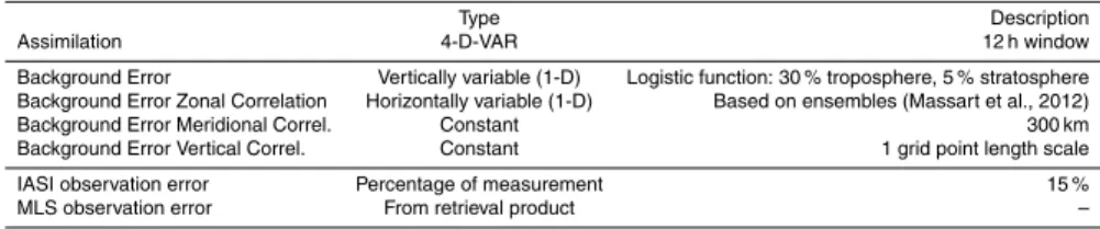
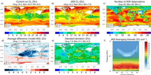
We computed the ozone field with a free run of the model (without DA, also named control run) in August/November 2008. The global average di_fference between this sim-ulation and the ozone-sondes profiles is displayed in Fig. 1. Differences are presented in term of bias and Root Mean Square Error (RMSE) components and normalized with an ozone climatological profile (Paul et al., 1998). The number and the geographical

25

(15)

ACPD

13, 21455–21505, 2013

E. Emili et al.

Title Page

Tables Figures

◭ ◮

Back Close

Full Screen / Esc

Discussion

P

a

per

|

D

iscussion

P

a

per

|

Discussion

P

a

per

|

Discuss

ion

P

a

per

the model free run has globally a small relative bias (<10%) except in November,

inside the Planetary Boundary Layer (PBL,p>750 hPa). The good free model

perfor-mances are partly due to the accurate initial conditions prescribed on the first day of each month, which come from the previous MLS analysis. The relatively long life-time of ozone (Sect. 3.1) implies that, assuming a good description of the transport, the

5

model error keeps memory of those conditions for several weeks. The RMSE profile in Fig. 1 shows that below 100 hPa the model total error increases up to about 30 %, with two higher peaks, one below the tropopause (_∼300 hPa) and the other in the PBL. Since the bias does not have such a distinct shape most of the RMSE error originates from the deficiencies of the model in reproducing the variability of measured ozone in

10

these two layers. This behavior is not surprising in the troposphere, and especially in the PBL, since detailed ozone tropospheric chemistry is not taken into account within the O₃ linearized chemistry scheme. Moreover, since the initial condition comes from MLS analysis, the model was not constrained by any observation in the troposphere. We remark also that there is no evidence of a strong monthly dependence of the error

15

profiles.

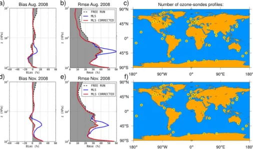
The parameter configuration used for the assimilation experiments presented in this and in the following sections is summarized in Table 1. Compared to the study of Mas-sart et al. (2012), the background error variance is given in percentage of the ozone field (Fig. 2) and the vertical correlation length is set to one vertical grid point. Since

20

the e_ffects of using an ensemble based variance were not found to be highly significant and no estimation was available in the troposphere from the cited study, this choice was made to have a time dependent background error variance across the whole at-mosphere. On the basis of the model free run validation (Fig. 1), we set a bigger uncer-tainty in the troposphere (30 %) than in the stratosphere (5 %). The choice of a small

25

(16)

ACPD

13, 21455–21505, 2013

E. Emili et al.

Title Page

Tables Figures

◭ ◮

Back Close

Full Screen / Esc

Discussion

P

a

per

|

D

iscussion

P

a

per

|

Discussion

P

a

per

|

Discuss

ion

P

a

per

|

et al. (2012) with a zonal and time-independent average for the zonal length scale Lx (Fig. 2) and a constant value of 300 km for the meridional length scale Ly. All these simplifications are not supposed to influence greatly the analysis, given the results in Massart et al. (2012).

The validation of the MLS analysis is also shown in Fig. 1. When all MLS

lev-5

els are used (Sect. 2) both the bias and the RMSE are reduced in the stratosphere (p<100 hPa) but enhanced at around 300 hPa. This local degradation of the analysis

was already observed in previous MLS assimilation studies (Stajner et al., 2008; Mas-sart et al., 2012). Since there is strong evidence of a positive bias for the lowermost MLS level (215 hPa) (Jackson, 2007; Froidevaux et al., 2008), this level was removed

10

from the assimilated dataset, leading to a better analysis (red line in Fig. 1). The strato-spheric RMSE is globally reduced to almost 10 % both in August and November 2008. These results confirm the findings of a number of already cited studies that assimilated MLS ozone with other models. Note that, even after the exclusion of the 215 hPa MLS level, the analysis ozone profile between 200 hPa and 300 hPa still di_ffers slightly from

15

the control run. Since the vertical error correlation was fixed to 1 grid point and there is approximately a 8 grid points separation between the lowermost assimilated level (140 hPa) and the aforementioned layer, those changes are imputable to the model dynamics, likely through downward ozone transport (STE).

4.2 IASI TOC column assimilation

20

IASI retrieved ozone, unlike MLS ozone, has not been used in many assimilation stud-ies. Therefore, a comparison between observations and the correspondent free model values allows a preliminary quantification of the scatter and the systematic biases be-tween the two. Later, the validation of the assimilated fields with independent data will provide further insights about biases with respect to “true” ozone values.

25

(17)

ACPD

13, 21455–21505, 2013

E. Emili et al.

Title Page

Tables Figures

◭ ◮

Back Close

Full Screen / Esc

Discussion

P

a

per

|

D

iscussion

P

a

per

|

Discussion

P

a

per

|

Discuss

ion

P

a

per

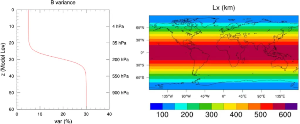
compensate known retrieval biases (Sect. 2). The impact of such a bias correction on the further assimilation is detailed later in this section. IASI tropospheric partial columns (TOC, 225–1000 hPa) are compared to the free model equivalent columns by means of the observation operator, thus taking into account the spatio-temporal colocation and the satellite averaging kernels. Maps show that in both seasons the model significantly

5

underestimates IASI partial columns at low latitudes (30◦S–30◦N) in the Middle East, Africa and Central/South America (bias as high as 10 DU, corresponding to∼100% of

model values). A smaller but positive bias (2–4 DU) is found at lower latitudes (30◦_S– 90◦S), which is however less significant compared to the greater local column amount. Average standard deviations are 2 DU (Dobson Units) for both seasons with maximum

10

values of about 5 DU localized between 30◦_S–60◦_{S and over desert regions (Saharan} and Australian deserts).

High systematic differences are found in regions dominated by dust aerosols, like the Atlantic ocean band east of the Saharan desert (Remer et al., 2008). Dust aerosols are known to reduce the accuracy of infrared ozone retrievals, like IASI ones. However, IASI

15

retrievals biases for the ozone total columns are normally lower than 30 % in presence of dust (Boynard et al., 2009) so that this cannot entirely explain the observed di_ff er-ences (as high as 100 %). Therefore the remaining systematic di_fferences are mostly attributed to the model deficiencies. Indeed, the model underestimates ozone in sev-eral regions a_ffected by biomass burning outflow, like eastern Africa in August, western

20

South America in November or in the western Indian Ocean (van der Werf et al., 2006; Barret et al., 2011). The reason for such biases is the model simplified tropospheric chemistry, which does not take into account emissions of ozone precursors and their impact on local ozone chemistry. This will be confirmed by the independent validation carried further in this section.

25

(18)

ACPD

13, 21455–21505, 2013

E. Emili et al.

Title Page

Tables Figures

◭ ◮

Back Close

Full Screen / Esc

Discussion

P

a

per

|

D

iscussion

P

a

per

|

Discussion

P

a

per

|

Discuss

ion

P

a

per

|

the atmospheric layers and the continental surface in summer, which enhances the DFS and the number of pixels that pass the AVK trace filter (Sect. 2). This is also the reason why the zonal averaging kernels (Figs. 3f and 4f), which depend mostly on the ocean–atmosphere thermal gradient, have a stronger peak during winter. Note that the low trace screening filters out most of the observations over ice and high altitude

sur-5

faces (e.g. Greenland, South Pole, Himalaya and Rocky mountains), which have a poor thermal contrast or not enough tropospheric pressure levels available. Finally, desert regions show also a decreased number of observations due to issues in correctly rep-resenting the sand emissivity in the infrared ozone retrieval.

Figure 5 shows the error profiles for the IASI TOC analysis. The initial condition

10

and the assimilation configuration are the same as in the MLS analysis (Sect. 4.1 and Table 1) but no MLS data are assimilated at this point. Using horizontal length scales previously diagnosed with MLS ensembles (Fig. 2) might not be pertinent for the troposphere. Nevertheless, IASI data coverage is very dense in space and time (Figs. 3 and 4) and the impact of the background error horizontal correlations is supposed to

15

be exiguous. This will also be illustrated later in the article (Sect. 4.3.1).

When IASI data are not bias-corrected the analysis is sometimes worse than the control run (Fig. 5): the tropospheric bias increases by 10–20 % for both months and the RMSE improves in August but deteriorates in November. Instead, when 10 % of the values is globally removed from IASI observations the bias of the analysis improves

20

or stays the same with respect to the control run and the RMSE is reduced by about 5–10 % in both months. The profile is corrected significantly only between 200 hPa and 800 hPa, where the AVK values are greater than 10 DU vmr−1 _{(Figs. 3 and 4).} Comparing the curves in Figs. 1 and 5 we conclude that with the selected value of the background error vertical correlation, the correction brought by the two instruments

25

(MLS and IASI) remains well separated vertically.

(19)

ACPD

13, 21455–21505, 2013

E. Emili et al.

Title Page

Tables Figures

◭ ◮

Back Close

Full Screen / Esc

Discussion

P

a

per

|

D

iscussion

P

a

per

|

Discussion

P

a

per

|

Discuss

ion

P

a

per

signal in this study. Neglecting the AVK information lead to significantly worse results (not shown), which demonstrates their importance in the vertical localization of the assimilation increments. Several assimilation experiments were done with a different definition of the TOC column, obtained by lowering the top height of the column to 300, 400 and 500 hPa. Since the AVK is spread above the specified column top height, this

5

was done to reduce the possible contamination of stratospheric air masses at high lat-itudes, which might introduce positive tropospheric ozone biases in the analysis. No significant improvements were however observed in any of these analyses.

4.3 MLS+IASI combined assimilation

In the previous sections MLS and IASI ozone products have been assimilated

sepa-10

rately during August and November 2008. The purpose was to test the assimilation algorithm and detect issues like observational biases, with the help of sondes data. In this section the combined assimilation of both instruments is detailed: still for the two months separately first, and for a simulation of 6 months (July–December 2008) later. In addition to the usual validation against sondes data, a comparison with OMI

15

total ozone columns and free troposphere in-situ measurements are reported. This will better clarify the added value of the IASI assimilation compared to the MLS on its own. Figure 6 depicts the error profiles (bias and RMSE) of the combined analysis for August and November 2008 and the zonal differences between the analysis and the control run. Since the increments due to the two instruments are quite separated

verti-20

cally, the error profile of the combined analysis is almost equivalent to the combination of the error profiles of the two separated analyses (Figs. 1 and 5). The zonal di_ff er-ences (Fig. 6c and f) show that the ozone concentration is increased by 20–30 % in the tropical region (30◦_S–30◦_{N) both in the troposphere and in the lower stratosphere,} and decreased by 10–20 % in the southern latitudes (30◦_S–90◦_{S) free troposphere}

25

(20)

ACPD

13, 21455–21505, 2013

E. Emili et al.

Title Page

Tables Figures

◭ ◮

Back Close

Full Screen / Esc

Discussion

P

a

per

|

D

iscussion

P

a

per

|

Discussion

P

a

per

|

Discuss

ion

P

a

per

|

tropospheric positive increment is slightly shifted toward the northern mid-latitudes in summer (40◦_{N). The average increments are able to correct most of the deficiencies of} the direct model, which are: (i) the lack of ozone precursors emissions and chemistry in the tropical/mid-latitudes troposphere and (ii) the presence of high-latitude strato-spheric positive biases due to a too strong polar-ward circulation in the forcing wind

5

field (Cariolle and Teyssedre, 2007; de Laat et al., 2007).

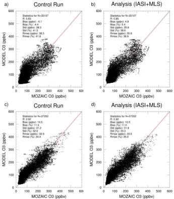
A complementary validation of the ozone fields obtained with the combined as-similation is provided by a comparison with MOZAIC data. These data allow a good geographical and temporal coverage in the Northern Hemisphere, due to the daily frequency of commercial flights, but with 90 % of the data vertically confined at the

10

airplane cruise altitude (∼200 hPa). Scatter plots between model ozone values and

MOZAIC observations above 400 hPa are reported in Fig. 7. Raw data were temporally averaged on a minute basis to better fit the model spatial resolution. Some data redun-dancy might still be present, even though the validation statistics are not supposed to be sensitive to that. Overall the relative error lies between 35 and 40 %. The scores are

15

very similar to those obtained using sondes data (Fig. 6, 200 hPa level) and highlight a modest improvement of the correlation and the RMSE for the IASI-MLS analysis in August and a slight worsening in November. Therefore we only consider sondes data hereafter.

Figure 8 shows the geographical di_fferences of the TOC among the control run and

20

the analysis. In addition to Fig. 6, which already highlighted the zonal features of the increments, we note a significant increase of the TOC over the African continent and the Atlantic region, whereas the local ozone minimum over Indonesia is not changed or even slightly decreased. This is consistent with the preliminary comparison between modeled and IASI ozone shown in Figs. 3 and 4. The main spatial features of the

25

(21)

ACPD

13, 21455–21505, 2013

E. Emili et al.

Title Page

Tables Figures

◭ ◮

Back Close

Full Screen / Esc

Discussion

P

a

per

|

D

iscussion

P

a

per

|

Discussion

P

a

per

|

Discuss

ion

P

a

per

et al., 2011). Hence, a more quantitative comparison would require the same definition of the TOC column to be adopted.

A quantitative comparison of the analysis with OMI total ozone columns is presented in Fig. 9. The comparison is done between independent averages of both datasets, which do not consider the exact temporal matching. Since OMI permits a daily global

5

coverage, differences due to this reason are assumed negligible. The greatest posi-tive correction originates from the assimilation of MLS data, which modify the more abundant stratospheric ozone. However, the addition of IASI TOC permits to reach the best agreement between the analysis and OMI data in the tropics, where the strato-spheric column amount is lower and the total ozone column is more sensible to the

10

tropospheric amount.

4.3.1 Sensitivity of the analysis to the background/observation error covariance

Before calculating the 6 months-long analysis, alternative formulations of the back-ground and the observation error covariance matrices have been tested to verify the robus tness of the analysis to the choice of the assimilation parameters. The following

15

cases have been considered, where the non-specified parameters are kept the same as in Table 1:

– temporally constant background variance expressed in ozone concentration units and derived from the MLS ensemble (Massart et al., 2012) above the tropopause (full 3-D field) and from sondes validation in the troposphere (zonally averaged

20

field, three latitude bands used);

– background variance equal to 20 % of the ozone field everywhere, constant and homogenous horizontal error length scale equal to 4◦;

– error statistics as in Table 1 but optimization of B and R matrix based on a-posteriori diagnostics (Sect. 3.2).

(22)

ACPD

13, 21455–21505, 2013

E. Emili et al.

Title Page

Tables Figures

◭ ◮

Back Close

Full Screen / Esc

Discussion

P

a

per

|

D

iscussion

P

a

per

|

Discussion

P

a

per

|

Discuss

ion

P

a

per

|

The first two represent two cases of more/less detailedBmatrix and the last one a case of statistical optimization ofBandRat the same time. In all cases the comparison with sondes profiles was not found to be superior or differences with the reference anal-ysis were not significant (not shown). The reasons are attributed to the combination of the high temporal frequency of the assimilated satellite observations and the

rel-5

atively slow ozone chemistry, which makes the background error strongly dependent on the initial condition. Once the model is corrected for the inexact initial conditions, further assimilation increments only bring minor adjustments, which keep the model close to the temporal trajectory of observations. This can be better clarified looking at the Observation minus Forecast (OmF) global statistics during the initial period of data

10

assimilation in the case of the long run experiment (Fig. 10). The initial condition is not issued from a previous MLS analysis in this case but comes from a 30 days model spin-up period. It follows that, compared to the case of the simulations for August and November 2008, the model field di_ffers initially more from the observations, especially the MLS ones. It takes approximately 3 days (6 assimilation windows) to reach the

15

forecast-model minimum for both the OmF average and standard deviation. The model forecast at 10 hPa, which is initially biased high by 1000 ppbv and has a standard devi-ation of 400 ppbv with respect to MLS measurements, reduces its bias to 100 ppbv and its scatter to 200 ppbv after 4 assimilation windows (48 h). In the case of IASI the bias and the scatter are reduced just after 24 h to∼0 DU for the bias and 1.5–2 DU for the

20

standard deviation from an initial value of 2 DU and 3 DU respectively. Subsequent val-ues of OmF are of the order of the prescribed observation errors, which are about 200– 300 ppbv for MLS 10 hPa level (Froidevaux et al., 2008) or 15 % of IASI TOC columns (Fig. 3), so that a further reduction is not possible. Note that IASI observations cover 80 % of the horizontal grid after 48 h, whereas MLS attains 40 % after 72 h (Fig. 10c).

25

This explains the faster convergence of IASI OmF statistics. In other words, observa-tions are dense enough to well constrain the long term (>5 days) temporal evolution

(23)

ma-ACPD

13, 21455–21505, 2013

E. Emili et al.

Title Page

Tables Figures

◭ ◮

Back Close

Full Screen / Esc

Discussion

P

a

per

|

D

iscussion

P

a

per

|

Discussion

P

a

per

|

Discuss

ion

P

a

per

trix. Different choices of the background covariance may determine the rapidity of the convergence during the initial assimilation windows.

4.3.2 Validation of the 6 months-long simulations

The 6 months-long assimilation experiment (analysis) is initialized with a free model spin-up of 1 month in June 2008. The assimilation starts on 1 July 2008 and ends on

5

31 December 2008. For the same period a simulation without data assimilation (control run) is calculated.

Figure 11 shows the Taylor diagram of the collocated model-sondes columns. The 6 months period allows to accumulate enough sondes profiles to validate the model sep-arately for different latitude bands. In addition to the TOC (1000–225 hPa), also the

Up-10

per Troposphere/Lower Stratosphere (UTLS, 225–70 hPa) column is considered. This type of plot depicts the capacity of the model to explain the variability of the validation dataset. In Figs. 12 and 13 columns/profiles bias, RMSE and standard deviation are also displayed to give a complete picture of the model performances. The results can be summarized as follows:

15

– Globally the UTLS column scores are significantly better for the analysis (R = 0.98, bias<1 %, RMSE _∼15 %) than for the control run (R=0.9, bias_∼15 %,

RMSE∼30 %);

– The control run shows in particular a very high UTLS error in the 90◦_S–60◦_{S band} (bias∼50 %, RMSE∼60 %), due to the linear chemistry limitations with regards

20

to the mechanism of ozone depletion;

– The TOC scores are also globally better for the analysis (R=0.7, bias < 5 %,

RMSE ∼20 %) than for the control run (R=0.6, bias ∼-10 %, RMSE∼ 25 %),

(24)

ACPD

13, 21455–21505, 2013

E. Emili et al.

Title Page

Tables Figures

◭ ◮

Back Close

Full Screen / Esc

Discussion

P

a

per

|

D

iscussion

P

a

per

|

Discussion

P

a

per

|

Discuss

ion

P

a

per

|

– All analysis TOC scores are significantly better than those of the control run at the tropics, but only the bias is substantially improved at northern mid-latitudes (from

−15% to<5%);

– In the 30◦S–60◦S and 60◦N–90◦N bands the TOC bias of the analysis field in-creases with respect to the control run. It follows that the analysis RMSE are not

5

improved and the Taylor diagram scores are unchanged or even deteriorated;

– The analysis TOC is particularly inaccurate in the 90◦_S–60◦_{S band (}_R =0.3,

bias _∼ 20 %, RMSE _∼ 25 %). However, the control run has already poor skills

and very few IASI observations are assimilated during the whole period (Figs. 3 and 4).

10

The good quality of the UTLS ozone analysis with MLS data confirm the findings of pre-vious studies (Jackson, 2007; El Amraoui et al., 2010; Massart et al., 2012). The results appear more heterogeneous with regards to the TOC analysis. The MLS-IASI assim-ilation has a robust and positive impact at low latitudes (30◦S–30◦N) which, however, becomes less evident at high latitudes and in polar regions. Other studies also

iden-15

tified di_fficulties in improving modeled tropospheric column at high latitudes by means of satellite data assimilation (Lamarque et al., 2002; Stajner et al., 2008). We conclude that IASI measurements, even if directly sensible to the tropospheric ozone concentra-tion, are not able to fill this gap. Since modeled TOC at high latitudes is quite accurate (RMSE∼20%, Fig. 12), we assume that IASI retrieval biases become too large

com-20

pared to model errors. Besides, the 10 % bias removed globally from IASI columns could have a zonal dependence, which was not considered in this study. However, ad-ditional validation studies of IASI products would be required to precisely assess this dependency.

Sondes data provide accurate information about the ozone vertical profile but their

25

(25)

ACPD

13, 21455–21505, 2013

E. Emili et al.

Title Page

Tables Figures

◭ ◮

Back Close

Full Screen / Esc

Discussion

P

a

per

|

D

iscussion

P

a

per

|

Discussion

P

a

per

|

Discuss

ion

P

a

per

selected sites are at the tropics (Mauna Loa, 19.54◦_{N, 155.58}◦_{W) and at high latitudes} (Summit, 75.58◦_{N, 38.48}◦_{W). Figure 14 shows the time series of the analysis, the} control run and the correspondent observations in August and November 2008. Since the ozone variability at very small spatial and temporal scales cannot be captured by a 2◦

×2◦ grid model, original hourly observations have been smoothed in time using

5

a moving average of±6 h.

The control run underestimates the temporal variability of observations, as expected from a model that does not account for tropospheric chemistry. The analysis field has an increased variability when compared to the control one, still maintaining its low bias. However, the scores in term of correlation and standard deviation between the

10

analysis time series and the observations (not shown) are not necessarily better than those of the control run. Note that at the Summit site and during August, the analysis is almost coincident with the control run because there are very few observations being assimilated in the surroundings (Fig. 3c).

This comparison leads to the conclusion that the assimilation of column integrated

15

information corrects well the model TOC (e.g. at the tropics, Figs. 12 and 11) but does not necessarily improve the model prediction at a single vertical level. IASI AVK re-distribute the satellite information in accordance with their vertical sensitivity and their a-priori, but the increments inside the partial column are still assigned proportionally to the model background profile. Hence, model predictions at a single vertical level do not

20

necessarily ensure the same accuracy as the one found for partial columns.

5 Conclusions

In this study we examined the impact of MLS and IASI (SOFRID product) ozone mea-surements to constrain the ozone field of a global CTM (MOCAGE) by means of varia-tional data assimilation and with particular emphasis on tropospheric ozone. Given the

25

(26)

cov-ACPD

13, 21455–21505, 2013

E. Emili et al.

Title Page

Tables Figures

◭ ◮

Back Close

Full Screen / Esc

Discussion

P

a

per

|

D

iscussion

P

a

per

|

Discussion

P

a

per

|

Discuss

ion

P

a

per

|

erage of IASI data is expected to make up for the deficiencies of the linear chemistry model used.

Results confirm the effectiveness of MLS profiles assimilation in the stratosphere, with an average reduction of RMSE with respect to ozone-sondes from 30 % (model free run) to 15 % (analysis) for the UTLS column. The lowermost level of MLS data

5

(215 hPa) was found to increase the analysis bias in the troposphere and is not further

used. Improvements of the tropospheric columns (TOC) due to IASI O₃ data

assim-ilation depend on the latitude and highlight the need to properly account for retrieval biases. When a globally constant 10 % positive bias is removed from IASI observa-tions, the TOC RMSE decreases from 40 % (model free run) to 20 % (analysis) in

10

the tropics and from 22 % to 17 % in the Northern Hemisphere (30◦_N–60◦_{N) whereas} it slightly increases (1–2 %) at other latitudes, probably due to residual IASI biases. Overall, the combined assimilation of MLS and IASI improves the correlations with ozone-sondes data for both the UTLS and TOC columns at almost all latitudes and increases the agreement with OMI total ozone column measurements. It is also found

15

that the analysis is not very sensible to the parametrization of the background error covariance, due to the high temporal frequency of IASI and MLS observations and the strong dependency of the ozone field on the initial condition. Finally a comparison with hourly-resolved in-situ measurements in the free troposphere shows that assimilating information with a coarse vertical resolution increases the model variability but does

20

not ensure a better hourly analysis at a particular vertical level.

We conclude that the assimilation of IASI and MLS data is very beneficial in combi-nation with a linear ozone chemistry scheme. The high frequency of IASI observations is able to make up for model simplified tropospheric chemistry, especially at low lati-tudes and also in regions affected by strong seasonal emissions of ozone precursors

25

(27)

precur-ACPD

13, 21455–21505, 2013

E. Emili et al.

Title Page

Tables Figures

◭ ◮

Back Close

Full Screen / Esc

Discussion

P

a

per

|

D

iscussion

P

a

per

|

Discussion

P

a

per

|

Discuss

ion

P

a

per

sors emissions and chemistry. However, IASI assimilation remains effective when the focus is on free-troposphere. Future applications of this system are the evaluation of tropopause ozone flux, a multi-annual climatology of global tropospheric ozone, anal-ysis of major pollution episodes and prescription of chemical boundary conditions for regional models. Possible improvements of the IASI analysis might be obtained by

as-5

similating IASI radiances directly into the CTM, thus considering a dynamical a-priori profile in the radiance inversion, instead of one issued from a climatology. Moreover, the development of a 4-D-VAR assimilation chain for the complete chemistry model will allow in future to consider the feedbacks of satellite ozone assimilation on other species.

10

Acknowledgements. This work was supported by the MACC, MACCII projects (funded by the European Commission under the EU Seventh Research Framework Programme, contract num-ber 218793), the ADOMOCA project (funded by the French LEFE INSU program) and the TOSCA program (funded by the French CNES aerospace agency). We thank NASA for pro-viding MLS and OMI satellite ozone products. OMI analyses used in this paper were produced

15

with the Giovanni online data system, developed and maintained by the NASA GES DISC. We acknowledge the Ether French atmospheric database (http://ether.ipsl.jussieu.fr) for providing IASI data and the NOAA ESRL Global Monitoring Division (http://esrl.noaa.gov/gmd) for pro-viding surface ozone measurements. We acknowledge for the strong support of the European Commission, Airbus, and the Airlines (Austrian-Airlines, Austrian, Air France) who carry free of

20

charge the MOZAIC equipment and perform the maintenance since 1994. MOZAIC is presently funded by INSU-CNRS, Meteo-France, and FZJ (Forschungszentrum Julich, Germany). We thank all the individual agencies that provided ozone-sondes data through the World Ozone and Ultraviolet Radiation Data Centre (WOUDC).

References

25

Ambrose, J., Reidmiller, D., and Jaffe, D.: Causes of high O3in the lower free troposphere over