www.the-cryosphere.net/10/2847/2016/ doi:10.5194/tc-10-2847-2016
© Author(s) 2016. CC Attribution 3.0 License.
Relating optical and microwave grain metrics of snow: the relevance
of grain shape
Quirine Krol and Henning Löwe
WSL Institute for Snow and Avalanche Research SLF, Flüelastrasse 11, 7260 Davos Dorf, Switzerland Correspondence to:Henning Löwe ([email protected])
Received: 13 May 2016 – Published in The Cryosphere Discuss.: 10 June 2016
Revised: 31 October 2016 – Accepted: 2 November 2016 – Published: 21 November 2016
Abstract.Grain shape is commonly understood as a morpho-logical characteristic of snow that is independent of the opti-cal diameter (or specific surface area) influencing its physiopti-cal properties. In this study we use tomography images to in-vestigate two objectively defined metrics of grain shape that naturally extend the characterization of snow in terms of the optical diameter. One is the curvature length λ2, related to the third-order term in the expansion of the two-point corre-lation function, and the other is the second momentµ2of the chord length distributions. We show that the exponential cor-relation length, widely used for microwave modeling, can be related to the optical diameter andλ2. Likewise, we show that the absorption enhancement parameterBand the asymmetry factorgG, required for optical modeling, can be related to the optical diameter andµ2. We establish various statistical re-lations between all size metrics obtained from the two-point correlation function and the chord length distribution. Over-all our results suggest that the characterization of grain shape viaλ2orµ2is virtually equivalent since both capture simi-lar aspects of size dispersity. Our results provide a common ground for the different grain metrics required for optical and microwave modeling of snow.
1 Introduction
Linking physical properties of snow to the microstructure always requires the identification of appropriate metrics of grain size. In this regard the two-point correlation function has become a key quantity for the prediction of various prop-erties such as thermal conductivity, permeability and electro-magnetic properties of snow (Wiesmann and Mätzler, 1999; Löwe et al., 2013; Calonne et al., 2014b; Löwe and
Pi-card, 2015). The two-point correlation function carries, in essence, information about a distribution of relevant sizes in the microstructure. For microwave applications, the analy-sis of two-point correlation functions was already used in the era before micro-computed tomography (µCT), where thin section data and stereology were employed to obtain the required information (Vallese and Kong, 1981; Zurk et al., 1997; Mätzler and Wiesmann, 1999). The recently gained in-terest in two-point correlation functions is mainly driven by available data fromµCT, from which the two-point correla-tion funccorrela-tion can be conveniently estimated. The relevance of the two-point correlation function for microwave modeling originates from the connection between its Fourier transform and the scattering phase function in the Born approximation for small scatterers (Mätzler, 1998; Ding et al., 2010; Löwe and Picard, 2015) or the connection to the effective dielectric tensor via depolarization factors (Leinss et al., 2016).
The exponential correlation length is often inferred from measurements of the optical equivalent diameter dopt or, equivalently, from the specific surface area (SSA). This link was established statistically (Mätzler, 2002), leading to the empirical relation
ξ ≈0.5dopt(1−φ), (1)
whereφis the ice volume fraction. This relation facilitates using the measured optical diameter as the primary input for microwave modeling (Durand et al., 2008; Proksch et al., 2015b; Tan et al., 2015). However, this link betweenξ and
doptcan only serve as a first approximation. The numerical prefactor in Eq. (1) seems to depend on snow type (Mätzler, 2002), which causes a significant scatter in estimating the exponential correlation length from optical diameter. This poses the question of which additional size metric captures variations in grain shape and explains the scatter.
A similar issue of grain shape emerges in the context of optical measurements. Optical properties (e.g., reflectance) can be largely predicted from the optical diameter or SSA (Kokhanovsky and Zege, 2004). The remaining scatter is commonly attributed to shape (Picard et al., 2009), which influences the absorption enhancement parameterB and the asymmetry factor gG (Kokhanovsky and Zege, 2004). The influence of grain shape onB for light penetration was re-cently addressed and measured by Libois et al. (2013, 2014). The question remains of which additional size metric of the microstructure can be used to capture variations in grain shape and measured scatter inB.
The two examples from microwave or optical modeling above reflect the known fact that the optical diameter as a single metric of grain size is not sufficient to characterize the microstructure for many physical properties. It is thus neces-sary to account for additional grain size metrics which imple-ment the idea of grain shape. A key requireimple-ment for poten-tial new shape metrics is a well-defined geometrical mean-ing. Present snowpack models (Vionnet et al., 2012; Lehn-ing et al., 2002) contain empirical shape descriptors such as sphericity (Brun et al., 1992). An objective definition of these quantities for arbitrary two-phase materials is, however, not possible. New shape metrics should thus ideally seek to re-place empirical parameters by an objective, measurable and geometrically comprehensible metric.
One appealing route to define shape is via curvatures of the ice–air interface because curvatures (i) have already been used to comprehend snow metamorphism via mean and Gaussian curvatures (Brzoska et al., 2008; Schleef et al., 2014; Calonne et al., 2014a), (ii) are natural quantities to as-sess shape via deviations from a sphere, very close to the definition of sphericity in Lesaffre et al. (1998), and (iii) nat-urally emerge as higher-order terms in the expansion of the two-point correlation function (Torquato, 2002). The latter fact can be used in turn to assess variations of the microwave parameter (ξ) from µCT images, which links back to the aforementioned microwave modeling problem.
Another appealing route to define shape is via chord length distributions because they (i) naturally implement the idea of size dispersity and (ii) have recently been put forward by Ma-linka (2014) to derive closed-form expressions for the aver-aged optical properties of a porous medium. Again, the latter fact can in turn be used to assess variations in the optical pa-rameters (gG,B) fromµCT images, which links back to the aforementioned optical modeling problem.
The motivation of the present paper is to investigate and interconnect these two routes of (objectively) defining grain shape. First, we will assess the curvature length in the expan-sion of the two-point correlation function. We will be guided by the questions of whether, and how, the well-known sta-tistical relation Eq. (1) between the exponential correlation length and the optical diameter can be improved by incor-porating curvatures. Second, we will characterize the mi-crostructure in terms of chord length distributions in order to make contact to aspects of shape in snow optics. An inter-connection between the two routes can be established by an approximate relation between the two-point correlation func-tion and the chord length distribufunc-tion that was originally sug-gested in the context of small angle scattering (Méring and Tchoubar, 1968). By means of this approximate relation we establish various statistical links between all involved size metrics, the moments of the chord length distributions, op-tical diameter, surface areas, curvatures and the exponential correlation length. The established links imply a microstruc-tural connection between geometrical optics and microwave scattering via size dispersity, which constitutes one aspect of grain shape.
The paper is organized as follows. In Sect. 2 we present the theoretical background for the two-point correlation func-tion, the chord length distribufunc-tion, the connection between both quantities and the governing length scales. In Sect. 3 we provide a summary of theµCT image analysis methods. To provide confidence of the interpretation of the curvature metrics derived from the two-point correlation function, we present an independent validation of these quantities via the triangulation of the ice–air interface. The results of the statis-tical models are presented in Sect. 4 and discussed in Sect. 5.
2 Theoretical background
2.1 Two-point correlation function and microwave metrics
0 for x in air. From that, a covariance function can be de-fined, which is often referred to as the two-point correlation function:
C(r)=I(x+r)I(x)−φ2. (2)
In the following we disregard anisotropy by stating thatC(r)
only depends on the magnitude ofr= |r|. To interpret snow with this approach, an average over different coordinate di-rections must be carried out.
The value of the two-point correlation function C(0)= φ (1−φ)is simply related to the volume fractions of ice and air. Therefore, often only the normalized two-point correla-tion funccorrela-tion is used (see Fig. 1b):
A(r)=C(r)/C(0). (3)
SinceA(r)must decay fromA(0)=1 to 0 forr→ ∞, the two-point correlation function is often described by an expo-nential form
A(r)=exp(−r/ξ ), (4)
in terms of the exponential correlation lengthξ. This single length scale empirically characterizes the decay ofA(r).
For small argumentsr, rigorous results for the decay of the correlation can also be inferred since the expansion ofA(r)
can be interpreted in terms of geometrical properties of the interface. According to Torquato (2002), the expansion for an isotropic medium reads
A(r)=1− r λ1
" 1− r
2
λ22+
O(r3)
#
(5)
in terms of the length scalesλ1andλ2. The first-order term 1
λ1
= − d
drA(r)
r=0
= s
4φ (1−φ) (6)
is the slope of the two-point correlation function at the origin and can be expressed in terms of the interfacial area per unit volumes(Debye et al., 1957). The size metricλ1is one of the most fundamental length scales for a two-phase medium and referred to as the “Porod length” in small angle scatter-ing, or “correlation length” in Mätzler (2002). We will ad-here to Porod length ad-here to clearly distinguishλ1from the exponential correlation lengthξ. The metricλ1can be also related to the SSA, defined as the surface area per ice mass (m2kg−1), or in turn to the equivalent optical diameterdopt of snow via
λ1=
4φ (1−φ)
s =
4(1−φ) ρiSSA
=2(1−φ)
3 dopt, (7)
withρi representing the density of ice. The last equality is obtained when the definition of dopt=6/ρiSSA is inserted (see Mätzler, 2002).
For a two-phase material with a smooth interface, the second-order term∼r2is missing in the expansion Eq. (5) and the next non-zero term is the cubic one with a prefactor 1/λ1λ22. Here the length scaleλ2has a geometric interpreta-tion in terms of interfacial curvatures and is therefore referred to as the curvature length hereafter. As originally shown by Frisch and Stillinger (1963), the following identity holds
1
λ22=λ1
d3 dr3A(r)
r=0
=1
8 H
2−K 3
!
(8)
in terms of the average squared-mean curvatureH2and the averaged Gaussian curvatureK. The quantityλ−22is propor-tional to the orientapropor-tionally averaged normal curvature of an interface (Tomita, 1986).
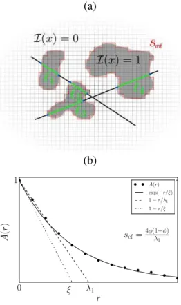
2.2 Chord length distributions and optical metrics In snow optics the microstructural characterization within ra-diative transfer theory (Kokhanovsky and Zege, 2004) com-monly involves a single metric, the optical diameter. An in-teresting approach for geometrical optics in arbitrary two-phase media was recently put forward by Malinka (2014). Thereby, the microstructure is taken into account by the chord length distribution of a medium which can be un-ambiguously defined for arbitrary two-phase random media (Torquato, 2002). Chord lengths in an isotropic medium are defined as the lengths of the intersections of random rays through the sample with the ice phase, as illustrated in the schematic in Fig. 1a. The chord length distributionp(ℓ)of the ice phase denotes the probability (density) for finding a chord of lengthℓ.
In contrast to the Born approximation for microwaves, where the microstructure enters as the Fourier transform of the two-point correlation function, the theoretical approach (Malinka, 2014) relates the key optical quantities (absorp-tion, phase func(absorp-tion, asymmetry factor) to the Laplace trans-form of the chord length distributionp(ℓ)which is denoted by
b
p(z)=
∞ Z
0
dℓ p(ℓ)e−zℓ (9)
with Laplace variablez. For smallz, the Laplace transform can be approximated by the expansion
b
p(z)=1−µ1z+ µ2
2 z
2+O(z3),
(10) whereµi denotes theith moment of the chord length distri-bution, viz.
µi= ∞ Z
0
(a)
(b)
0
r
1
A
(
r
)
λ1 ξ
scf=4φ(1 −φ)
λ1
A(r) exp(−r/ξ) 1−r/λ1
1−r/ξ
Figure 1. (a)Illustration of the chord lengths obtained from an ice sample. The mean chord length is defined as the average length of the green line lengths. A stereological approach (Underwood, 1969) to calculatesis to count the number of blue dots per unit length. The estimation forsmfis given by the red contour.(b)Illustration of the two-point correlation function A(r)and the method obtaining an estimate for the Porod lengthλ1to getscfby fitting the slope at the origin, and the exponential correlation lengthξ by fittingA(r)to
exp(−r/ξ )over a larger span.
Hence, within the approach from Malinka (2014), the optical response of snow can be systematically improved by succes-sively including higher moments of the chord length distri-bution. According to Malinka (2014), the Laplace transform has to be evaluated atz=α, with the absorption coefficient
α=4π κ/λ. Hereλ is the wavelength andκ the imaginary part of the refractive index of ice. It is generally sufficient (Malinka, 2014) to retain only a few terms in Eq. (10). It is straightforward to show (Underwood, 1969) that the first moment, i.e, the mean chord lengthµ1, is given by
µ1= 4φ
s =
λ1 1−φ =
2
3dopt (12)
and thus related to the surface area per unit volumes from Eq. (6), or the optical diameterdoptvia Eq. (7). Therefore, in lowest order, the Laplace transform Eq. (9) only contains the Porod length or specific surface area of snow. The next or-der correction involves the second momentµ2for which no geometric interpretation has been hitherto given for arbitrary two-phase random media.
For known chord length distribution, all optical quantities (phase function, single scattering albedo, etc.) can be directly computed from Malinka (2014). To make contact to other ap-proaches, for example Libois et al. (2013), and discuss our re-sults for the chord lengths in light of shape, an expression of the absorption enhancement parameterB is required within the framework of Malinka (2014), which is derived in Ap-pendix A. From these expressions we can asses the relative importance of theµ2correction to the optical diameterµ1. 2.3 Connection between chord lengths and the Porod
length and the curvature length
Following the previous two sections, a link between opti-cal and microwave metrics of snow thus requires to estab-lish a link between two-point correlation functions and chord length distributions. To this end we employ a relation be-tween the two-point correlation function and chord length distribution that was put forward in the early stages of small angle scattering (Méring and Tchoubar, 1968) to interpret the scattering curve in terms of particle properties. In the present notation the relation can be written as
p(ℓ)=µ1 d2
dℓ2A(ℓ), (13)
which was also used by Gille (2000).
Although Eq. (13) is only valid under certain assump-tions which will be discussed in Sect. 5, it has already some non-trivial implications that can be exploited for the subse-quent analysis. As a first consistency check of the approx-imation Eq. (13), we can compute the first moment of the chord length distribution from Eq. (11) forn=1 by inserting Eq. (13) and integrating by parts. This yieldsµ1=µ1A(0), which is correct by virtue of Eq. (3). As a next step, we aim at an expression for the second moment of the chord length dis-tribution in terms of interfacial curvatures by using Eq. (11) forn=2. Again, inserting Eq. (13) and integrating by parts yields
µ2=2µ1 ∞ Z
0
A(r)dr=2µ1f (φ, λ1, λ2, . . .). (14)
Thoughf is an unknown function here, this link shows that the chord length metricµ2must be somehow related to the two-point correlation function metricsλ1andλ2. In Sect. 4 we will statistically investigate the dependence off on its arguments.
3 Methods 3.1 Data
et al. (2013) for a thermal conductivity analysis and Löwe and Picard (2015) for a comparison of microwave scattering coefficients. All samples were classified according to Fierz et al. (2009) as described in the supplement of Löwe et al. (2013). The data set comprises 167 different samples includ-ing two time series of isothermal experiments, four time se-ries of temperature gradient metamorphism experiments and a set of 37 individual samples. In total, the set includes 62 samples of depth hoar (DH), 54 of rounded grains (RG), 33 of faceted crystals (FC) 10 of decomposing and fragmented precipitation particles (DF), 5 of melt forms (MF) and 3 of precipitation particles (PP).
3.2 Geometry from two-point correlation functions Obtaining the normalized two-point correlation function
A(r)from aµCT image can be conveniently done by using the fast Fourier transform (FFT) as, for example, described in Newman and Barkema (1999). The FFT is typically used for performance issues to evaluate the convolution integral Eq. (2) since direct methods can be very slow. The spatial resolution of the two-point correlation function depends on the voxel size1of theµCT image which ranges from 10 to 50 µm.
Since the snow samples in the data set are anisotropic (Löwe et al., 2013), the normalized two-point correlation function is first obtained in thex,yandzdirection and then averaged arithmetically over the three directions, i.e.,A(r)=
Ax(r)+Ay(r)+Az(r)/3.
From the normalized two-point correlation function two types of parameter fittings are performed. First, the exponen-tial correlation lengthξ is obtained by fitting theµCT data to the exponential form Eq. (4). Technically, we estimated the inverse parameterkby least-squares optimization of the model A(r)=exp(−kr)to the data in a fixed range of 0< r <501. An illustration of this method is shown in Fig. 1b. In the following we denote byξthe inverse of the optimal fit parameter ξ:=1/ k. Secondly, we estimated the expansion parametersλ1 andλ2 of the two-point correlation function by a least-squares regression to the expansion Eq. (5). Tech-nically, we fittedA(r)=1−k1r(1−k2r2)in the fixed range of 0< r <31, which determines the derivatives at the ori-gin. We denote byλcf1 andλcf2 the inverse of the optimal fit parameters λcf1 :=1/k1 and λcf2 :=1/k2. The superscript is added to discern these two-point correlation-function-based estimates from those presented in the next section for a vali-dation. The influence of resolution and anisotropy to the es-timates ofλ1andλ2is discussed in Sect. 5.
3.3 Geometry from triangulations
To confirm the geometrical interpretation ofλcf1 andλcf2 we use an alternative and independent method to estimate these parameters by measuring the surface area and the local curva-tures with a VTK-based image analysis as described in Krol
and Löwe (2016). In short, a triangulated ice–air interface is obtained by applying the VTKContour filter. After this step, the interface still resembles the underlying voxel struc-ture. Therefore, in a second step the triangulated interface is smoothed by applying the VTKSmoothing filter, which involves a smoothing parameterS that is the number of it-erations a Laplacian smoothing on a mesh is repeated. For further details we refer to Krol and Löwe (2016).
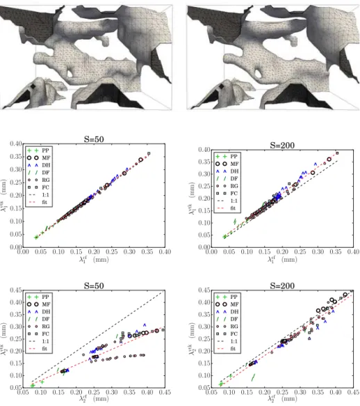
3.4 Accuracy of surface area and curvatures estimates The measured total surface area is obtained by integrat-ing (summintegrat-ing) the surface area of the triangles over the surface and the estimateλvtk1 , which naturally depends on the smoothing parameter. A comparison of the triangulation and the two-point correlation-function-based length scale is shown in Fig. 2 (middle row). A higher value of the smooth-ing parameter implies a lower surface area s (caused by shrinking of the enclosed volume upon smoothing) and in turn higher estimates forλvtk1 . Using higher smoothing also results in a higher variance in the data. This is likely due to filtering of small perturbations in the surface causing the in-dividual samples to react differently.
It is illustrative to note that even without smoothing for
S=0 the obtained triangulated surface is still different from the voxel surface smf, which is obtained by the union of ice–air transition faces in the voxel-based image (as illus-trated by the red contour in Fig. 1a). The quantitysmfis one of the four Minkowski functionals and can be computed by standard counting algorithms (Michielsen and Raedt, 2001). For isotropic systems, as well as statistically representative samples, the relation between the surface obtained from the two-point correlation functionscf=4φ (1−φ)/λcf1 and the Minkowski functionals is known to bescf=2smf/3 as dis-cussed in Torquato (2002, p. 290).
An estimate for the curvature-lengthλvtk2 is obtained from the VTKCurvature filter on the triangulated ice–air interface yielding local values for mean and Gaussian curvature which can be integrated to computeλvtk2 via Eq. (8). The compari-son of the triangulation-based curvature length and the two-point correlation-function-based curvature length is shown in Fig. 2 (bottom row). Again,λvtk2 depends strongly on the smoothing parameterS. The valueS=200 performed best by comparing the valueλcf2 toλvtk2 ; see Fig. 2 (bottom row). The deviations from the 1:1 line are caused by the over-estimation of the curvatures by the remaining steps in the triangulation from the underlying voxel-based data and is thus negatively correlated with the size of the structures and the resolution. In the end, we chose a smoothing parameter
S=200 that is, on average, acceptable for all involved sam-ples.
0.00 0.05 0.10 0.15 0.20 0.25 0.30 0.35 0.40
λcf
1 (mm)
0.00 0.05 0.10 0.15 0.20 0.25 0.30 0.35 0.40
λ
v
tk 1
(mm
)
S=50
PP MF DH DF RG FC 1:1 fit
0.00 0.05 0.10 0.15 0.20 0.25 0.30 0.35 0.40
λcf
1 (mm)
0.00 0.05 0.10 0.15 0.20 0.25 0.30 0.35 0.40
λ
v
tk 1
(mm
)
S=200
PP MF DH DF RG FC 1:1 fit
0.05 0.10 0.15 0.20 0.25 0.30 0.35 0.40 0.45
λcf
2 (mm)
0.05 0.10 0.15 0.20 0.25 0.30 0.35 0.40 0.45
λ
v
tk 2
(mm
)
S=50
PP MF DH DF RG FC 1:1 fit
0.05 0.10 0.15 0.20 0.25 0.30 0.35 0.40 0.45
λcf
2 (mm)
0.05 0.10 0.15 0.20 0.25 0.30 0.35 0.40 0.45
λ
v
tk 2
(mm
)
S=200
PP MF DH DF RG FC 1:1 fit
Figure 2.Comparison between smoothing parameterS=50 (left) andS=200 (right). Top: representation of the triangulated surface of a subsection of a snow sample. Middle: scatterplots of the Porod lengthλcf1 versusλvtk1 , including a fit (red dotted line). Bottom: scatterplots of the curvature-lengthλcf2 versusλvtk2 , including a fit (red dotted line).
the following we solely use the quantities derived from the two-point correlation function, viz. λ1=λcf1 and λ2=λcf2, where the superscripts are omitted for brevity.
3.5 Chord length distribution
To compute the ice chord length distribution from the bi-nary images, alllinear lines through the sample in all three Cartesian directions β=x,y,zare considered andallice chords were measured and binned to obtain direction depen-dent counting densities nβ(ℓ). Herenx(ℓ)denotes the total number of chords inx direction, which have lengthℓ. For a binary CT image,ℓcan take integer values 0< ℓ < Lxwhich are restricted by the sample size Lx=Nx1and the voxel size1of the image. The mean chord length and other mo-mentsµi are then computed from
µi= 1 P
ℓ,βnβ(ℓ) X
ℓ,β
ℓinβ(ℓ). (15)
3.6 Statistical models
4 Results
4.1 Relating exponential correlation length to the Porod length and curvature length
As a starting point for the statistical analysis we revisit the empirical relation
ξ =0.75λ1, (16)
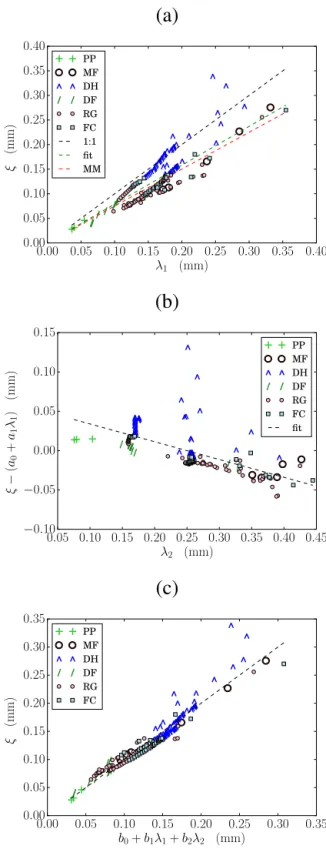
which is equivalent to Eq. (1) by virtue of Eq. (7), as sug-gested by Mätzler (2002). To this end we fitted ξ andλ1 and obtained an average slope of 0.79 with a correlation co-efficient of R2=0.733, shown by the green dashed line in Fig. 3a. In the next step we fitted the same data to include an intercept parameter
ξ =a0+a1λ1. (17)
Here the adjusted correlation coefficient, accounting for the inclusion of extra parameters, isR2=0.731 and the pa-rameters are given bya0=5.93×10⁻²mm anda1=0.794, with very lowpvalues (p <5×10⁻⁴) for the intercept and the slope ensuring the significance of the parameters of the fit. The order of magnitude of the intercept a0 is negligi-ble. To understand the remaining scatter we have plotted the residualsξ−(a0+a1λ1)versus the curvature-lengthλ2 as shown in Fig. 3b. The correlation coefficient is given by
R2=0.644 and suggests that including the curvature lengths can improve Eq. (17). For an overview, this and all other sta-tistical models are listed in Table 1.
In the next step we include the curvature-lengthλ2where we fitted the exponential correlation lengthξ to the model
ξ =b0+b1λ1+b2λ2. (18)
The results are shown in Fig. 3c. Here we find an improve-ment compared to Eq. (17). The correlation coefficient is
R2=0.922 and the fit parameters are given byb0=1.23× 10⁻²mm,b1=1.32 andb2= −3.85×10⁻¹. Thep values are very small for all coefficientsbi. The order of magnitude of the improvement can already be roughly estimated from the ratio of the prefactorsb1andb2.
4.2 Connection between chord length distributions and two-point correlation functions
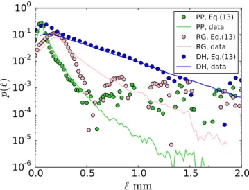
To relate the chord length metrics to the Porod length and the curvature length, we first assessed the relation between the chord length distributionp(ℓ)and the two-point correlation functionA(ℓ)as suggested by Eq. (13). To this end we com-pared the chord length distribution obtained directly from the
µCT image (cf. Sect. 3.5) with the prediction of Eq. (13) via the two-point correlation function for a few examples of dif-ferent snow types. The results are shown in Fig. 4. The se-lected snow samples are the same as those used in Löwe and Picard (2015, Figs. 8 and 9). Qualitatively, the characteristic
(a)
0.00 0.05 0.10 0.15 0.20 0.25 0.30 0.35 0.40
λ1 (mm) 0.00
0.05 0.10 0.15 0.20 0.25 0.30 0.35 0.40
ξ
(m
m
)
PP MF DH DF RG FC 1:1 fit MM
(b)
0.05 0.10 0.15 0.20 0.25 0.30 0.35 0.40 0.45
λ2 (mm)
−0.10 −0.05
0.00 0.05 0.10 0.15
ξ
−
(
a0
+
a1 λ1
)
(m
m
)
PP MF DH DF RG FC fit
(c)
0.00 0.05 0.10 0.15 0.20 0.25 0.30 0.35
b0+b1λ1+b2λ2 (mm) 0.00
0.05 0.10 0.15 0.20 0.25 0.30 0.35
ξ
(m
m
)
PP MF DH DF RG FC
Figure 3.Scatterplots of(a)the exponential correlation lengthξ
Figure 4.Comparison of the chord length distributions computed from Eq. (13) (symbols) and by direct analysis of the µCT data (solid line) for three examples of snow types (PP, RG and DH).
form (i.e., single maximum), the location of the maximum and the width of the distribution are correctly predicted by Eq. (13). However, there are obvious shortcomings, such as the oscillatory tail for the RG example when the chord length distribution is derived via Eq. (15). We will revisit these char-acteristics in the discussion.
4.3 Relating the second moment of the chord length distribution to the Porod length and the curvature length
Using the previous results we can derive an approximate re-lation between the second moment of the chord length distri-bution and the interfacial curvatures. To motivate a statistical model, we start from Eq. (14):
µ2 2µ1
=f (φ, λ1, λ2, . . .) . (19)
We investigate the dependency of the functionf on parame-tersλ1,λ2andφof this expression by successively including λ1,λ2andφin a statistical model. In a first step we approxi-matef by a statistical model including onlyλ1:
µ2 2µ1
=l0+l1λ1. (20)
The optimal parameters for model Eq. (20) arel0= −2.40× 10⁻²mm andl1=1.25, with negligiblepvalues and a cor-relation coefficient ofR2=0.898. The results are shown in Fig. 5a.
In view of the inclusion of the curvature-lengthλ2, we ana-lyzed the residuals of the previous statistical model and plot-ted them as a function ofλ2(Fig. 5b). The correlation coef-ficient (R2=0.295) is small but includingλ2in the analysis further improves the fit. The respective statistical model
µ2 2µ1
=n0+n1λ1+n2λ2 (21)
(a)
0.00 0.05 0.10 0.15 0.20 0.25 0.30 0.35 0.40 0.45
l0+l1λ1 (mm)
0.00 0.05 0.10 0.15 0.20 0.25 0.30 0.35 0.40 0.45
µ2
/
(2
µ1
)
(m
m
)
PP MF DH DF RG FC 1:1
(b)
0.05 0.10 0.15 0.20 0.25 0.30 0.35 0.40 0.45
λ2 (mm)
−0.06 −0.04 −0.02
0.00 0.02 0.04 0.06 0.08
µ1
/
(2
µ1
)
−
(
l0
+
l1
λ1
)
(m
m
) PPMF
DH DF RG FC fit
(c)
0.00 0.05 0.10 0.15 0.20 0.25 0.30
q0+q1λ1+q2λ2 (mm)
0.00 0.05 0.10 0.15 0.20 0.25 0.30
(1
−
φ
)
µ2
/
(2
µ1
)
(m
m
)
PP MF DH DF RG FC 1:1
Figure 5. Scatterplots of (a) the statistical model see Eq. (20) predicting µ2/2µ1 depending on the Porod length λ1; (b) the residuals ofµ2/2µ1and the statistical model Eq. (20) versus the curvature-length scale parameterλ2;(c)the statistical model pre-dicting(1−φ)µ2/2µ1(see Eq. 22) depending on the Porod length
yields optimal parametersn0= −3.95×10⁻³mm,n1=1.50 andn2= −2.46×10⁻¹ with a correlation coefficientR2= 0.949. Thepvalue for the interceptn0is 0.36. Forn1andn2 thepvalues are again very low.
We have heuristically found a possibility of improving Eq. (21) even further. This was achieved by including a factor
(1−φ)on the left-hand side. More precisely, we tried
(1−φ)µ2 2µ1
=q0+q1λ1+q2λ2 (22)
as a statistical model. Here the optimal parameters areq0=
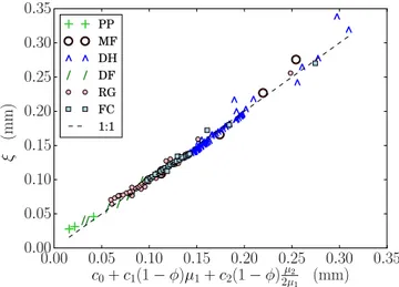
−1.23×10⁻²mm, q1=1.03 and q2= −1.98×10⁻¹. The pvalues for all coefficients are negligible and the correlation coefficient isR2=0.980. The results are shown in Fig. 5c. 4.4 Relating microwave metrics and optical metrics In the previous sections we found a statistical relation be-tween the exponential correlation lengthξand the geometri-cal lengthsλ1andλ2on one hand and a relation between the first and second moment of the chord length distribution (µ1 andµ2) andλ1andλ2on the other hand. Both findings can be recast into a direct connection between the moments of the chord lengthsµ1andµ2and the exponential correlation lengthξ. We express this relation in the statistical model
ξ =c0+c1(1−φ)µ1+c2
(1−φ)µ2 2µ1
. (23)
Note that(1−φ)µ1=λ1by virtue of Eq. (12), which means that we essentially replaceλ2by(1−φ)µ2/2µ1in the sta-tistical model Eq. (18) that relates ξ to λ1 and λ2. We obtained the correlation coefficient R2=0.985 for the op-timal parametersc0=9.28×10⁻³mm,c1= −7.53×10⁻¹ andc2=2.00. This final relation, Eq. (23), significantly im-proves both models Eq. (17) and Eq. (18).
The summary of all models is given in Table 1. To ensure that the inclusion of an additional parameter, for example by going from model Eq. (17) to model Eq. (18), is indeed an improvement, we have employed the Akaike information cri-terion (AIC) (Akaike, 1998). The AIC measure allows us to discern whether the improvement of the correlation coeffi-cient is trivially caused by an increasing number of fit pa-rameters or an actual improvement on the likelihood of the fit due to the relevance of the added parameters. Absolute AIC measures have no direct meaning, but a decrease of at least 2kbetween two models, wherekis the number of extra parameters, implies a statistical improvement. For our case
k=1 the difference in the AIC measure between Eq. (17) and Eq. (18) is 177, confirming the statistical relevance sig-nificance ofλ2.
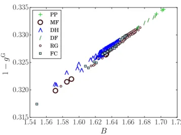
4.5 Shape factorsgGandB
As an application of the values obtained for the moments of the chord length distribution we can now compute the
0.00 0.05 0.10 0.15 0.20 0.25 0.30 0.35
c0+c1(1−φ)µ1+c2(1−φ)2µµ21 (mm)
0.00 0.05 0.10 0.15 0.20 0.25 0.30 0.35
ξ
(m
m
)
PP
MF
DH
DF
RG
FC
1:1
Figure 6.Scatterplot of the exponential correlation lengthξversus the statistical model Eq. (23) that depends on the first and second moment of the chord length distribution,µ1andµ2.
“shape diagram” of the optical parameters (gG, B) sug-gested in Libois et al. (2013) (derived from Malinka, 2014, Eq. 60 and Eq. (A4). The results depend on the value of the Laplace transform at the absorption coefficientαand thus on wavelengths. For most wavelengths in the visible and near-infrared regimeαµ1≪1 is small and therefore the Laplace transform Eq. (9) can be approximated by a few terms in the expansion Eq. (10). Taking typical values for α allows us to estimate the relative importanceαµ2/2µ1of the second-order term compared to the first-second-order term in the expansion Eq. (10). These values are obtained by using the values forκ
provided by Warren and Brandt (2008). The first-orderαµ1 and ratioαµ2/2µ1are calculated for typical wavelengths and shown in Table 2. The values and standard deviations denote averages taken over all samples. Wavelengths are selected to match common optical methods, namely 0.9 µm (Matzl and Schneebeli, 2006), 1.31 µm (Arnaud et al., 2011) and the shortwave infrared wavelengths 1.63, 1.74 and 2.26 µm used by Domine et al. (2006). We added the wavelength 2.00 µm, which is not used by any instrument but has the highest value forαin this range. Note that for this wavelengthαµ1is not small and the expansion of the Laplace transform, Eq. (10), likely not a good approximation. The standard deviations are high as a result of the variations due to grain type. The lowest values ofαµ2/2µ1are found for fresh snow (PP) and highest for DH and MF.
Table 1.Summary of statistical models.
Model Eq. Parameters (in order) (adj.)R2
ξ=a0+a1λ1 (17) 5.93×10⁻²mm, 0.79 0.731
ξ=b0+b1λ1+b2λ2 (18) 1.23×10⁻²mm, 1.32,−3.85×10⁻¹ 0.922
ξ=c0+c1(1−φ)µ1+c2(1−φ)µ2/2µ1 (23) 9.28×10⁻³mm,−7.53×10⁻¹, 2.00 0.985
µ2/2µ1=l0+l1λ1 (20) −2.40×10⁻²mm, 1.25 0.898
µ2/2µ1=n0+n1λ1+n2λ2 (21) −3.95×10⁻³mm, 1.50,−2.46×10⁻¹ 0.949
(1−φ)µ2/2µ1=q0+q1λ1+q2λ2 (22) +1.23×10⁻²mm, 1.03,−1.98×10⁻¹ 0.980
Table 2.Determination of the absorption coefficientα(Warren and Brandt, 2008), the first order, the fraction of the first and second order of Eq. (10) and the obtained estimates forBandgGaveraged over all snow samples, including the standard deviationσ.
Wavelength(µm) α(m−1) αµ1±σ µ2/2µ1α±σ (%) B 1−gG
0.90 4.1 0.00094±0.0003 <0.5 1.71±0.00 0.323±0.000 1.31 1.2×10² 0.026±0.008 2±1 1.64±0.02 0.316±0.000 1.63 2.0×10³ 0.45±0.14 37±13 0.89±0.20 0.253±0.011 1.74 1.1×10³ 0.24±0.079 20±7 1.19±0.14 0.272±0.010
2.00∗ 9.4×103 2.1±0.68 172±60 – –
2.26 1.1×10³ 0.25±0.08 20±7 1.14±0.13 0.240±0.010
∗Wavelength is not used for optical measurements
1.54 1.56 1.58 1.60 1.62 1.64 1.66 1.68 1.70 1.72 B
0.315 0.320 0.325 0.330 0.335
1
−
g
G
PP
MF
DH
DF
RG
FC
Figure 7.Scatterplot of (one minus) the asymmetry factorgGand the optical shape factorBevaluated for the refractive index at wave-lengthλ=1.3 µm.
wavelengths for which the shape signature might be higher but the expansion of Eq. (10) is less reliable. The results are averaged over all snow samples and included in Table 2.
5 Discussion 5.1 Methodology
Before turning to the discussion of physical implications of the results, we first address methodological details.
Retriev-ing parameters fromµCT images must be taken with care. In addition to the uncertainties related to filtering and segmen-tation pointed out by Hagenmuller et al. (2016), the present method also requires us to discuss the interface smoothing for the validation ofλ1andλ2, the image resolution and the anisotropy of the samples.
5.1.1 Geometrical interpretation
The present analysis and cross validation of the curvature metric imposes requirements on the smoothness of the inter-face. The subtle influence of the smoothing parameter on the surface areasand averaged mean and Gaussian curvaturesH
andKis apparent from Fig. 2. Naturally,H2is most sensi-tive to smoothing. We found a competing performance ofλ1 andλ2 with the smoothing parameter when comparing the triangulation-based estimates with the two-point correlation-function-based values. The agreement for the surface area seems to be best with smoothing parameterS=50. In con-trast, more smoothing is required to obtain an agreement for the curvature length. This higher sensitivity on the smooth-ing parameter is reasonable, since curvatures are defined by surface gradients which are more sensitive to a smooth mesh representation than the surface area. The competing behav-ior is caused by the smoothing filter, which preserves nei-ther the volume nor the surface area of the enclosed ice upon smoothing iterations. This causes the drop in agreement for
volume (Kuprat et al., 2001). Such problems could be partly avoided by computing normal vector fields and curvatures directly from voxel-based distance maps (Flin et al., 2005). A detailed comparison of all these different methods, how-ever, is beyond the scope of this paper. In contrast to λ1 and λ2, the interpretation of first and second moments of the chord length distribution, µ1 andµ2, is rather straight-forward, whereµ1is directly related to the optical diameter dopt, andµ2is a measure of the variations of this size metric. 5.1.2 Resolution
Resolution plays an important role in obtaining estimates for
λ1andλ2. For aµCT measurement the resolution is com-monly chosen appropriately depending on snow type. While fresh snow (PP) is typically reconstructed with 10 µm voxel size, MF and larger particles have larger voxel sizes of 35 µm or 54 µm. Since we have obtainedλ1andλ2with two inde-pendent methods that agree reasonably well we conclude that the resolution is generally sufficient to estimate the involved length scales. To further confirm that there is no remaining bias with resolution we assessed the ratioλ2/voxelsize. For our data, this ratio is 9.8 on average, with a standard de-viation of 2.6 and no systematic difference between small and large voxel sizes, implying thatλ2can be considered as equally well resolved for all snow samples.
The image resolution plays another important role in the interpretation of the expansion of the two-point correlation function. As pointed out by Torquato (2002), a missingr2
term is generally equivalent to a smooth interface while dis-continuities, like sharp edges, would lead to a second-order term. Fresh snow and depth hoar crystals are known to have these discontinuities, at least visually. However, it remains questionable if these features can be detected objectively at the micrometer scale from image analysis. In an image, dis-continuities are always smeared out, virtually contributing to the third-order term.
5.1.3 Anisotropy
The present data set was previously used to study the anisotropic properties of snow (Löwe et al., 2013). There-fore it is necessary to elaborate on the impact of anisotropy in the present analysis which exclusively involves isotropic two-point correlation functions. It is important to note that the our analysis does notassumeisotropy; it rather includes the orientational averaging in the three Cartesian directions as a part of the method. Such a procedure is principally valid for arbitrary samples. Moreover, also the geometrical inter-pretation of the quantities remains valid. This was rigorously shown for λ1 (Berryman, 1998) which relates the slope of the two-point correlation function at the origin for arbitrary anisotropic structures after orientational averaging to the sur-face area per unit volumes. Though we did not find a math-ematical proof for the corresponding statement for λ2, the
agreement of λcf2 (obtained from the two-point correlation function, orientationally averaged) withλvtk2 (obtained from direct computation of the interfacial curvatures) strongly sug-gests its validity. In addition, we assessed that the residuals betweenλvtk2 (where anisotropy does not play a role) andλcf2
are not correlated with anisotropy (R2=0.03).
Overall, we are confident that the method can be applied to arbitrary anisotropic samples to provide orientationally aver-aged length scales with the correct geometric interpretation with acceptable uncertainties due to image resolution. 5.2 Linking size metrics in snow
Accepting the methodological uncertainties, we shall now discuss our findings of the statistical analysis and their rel-evance for the interpretation of snow microstructure. 5.2.1 Including size dispersity to estimate the
exponential correlation length
By construction, the exponential correlation lengthξ must be understood as a proxy to characterize the entire two-point correlation function with a single length scale. This single length scale contains signatures of both properties that dom-inate the behavior of the two-point correlation function for small arguments (λ1andλ2) and other properties that dom-inate the tail behavior of the two-point correlation function for large arguments.
To discuss the statistical relations we will start with re-covering Mätzler’s model (Mätzler, 2002). This statistical model covers a relation between the exponential correlation length and the optical grain size, or in their nomenclature, the correlation length. Mätzler’s model predicts the slope to bea1=0.75, which is an average ofa1=0.8 for depth hoar anda1=0.6 for other snow types. This is consistent with our findinga1=0.79 since we have many depth hoar samples in the data set, suggesting that grain shape has a direct influence on the statistical relation. This influence was made quantita-tive by including the curvature length to the statistical anal-ysis, resulting in the statistical model Eq. (18) (Fig. 3c). The quantitative improvement on the statistical model Eq. (16) by using Eq. (18) is given by the increase in the correlation coefficient fromR2=0.733 toR2=0.922.
In addition we established a new statistical relation Eq. (23) betweenξ and the moments of the chord length dis-tribution,µ1andµ2. This model performs even better when the correlation coefficient R2=0.985 is taken as a quality measure. We confirmed that the inclusion of an additional pa-rameter in Eq. (18) and Eq. (23) indeed improves on Eq. (16), by employing the AIC measure (Akaike, 1998).
and Eq. (12), the two other size metricsµ2orλ2are the ori-gin of performance increase.
This seems surprising at first sight. Why should local as-pects of the interface (λ1 andλ2) determine the non-local decay of structural correlations (ξ)? To illustrate our expla-nation for this finding, we resort to a particle picture and con-sider a dense, random packing of monodisperse hard spheres. For such a packing, the particle “shape” is trivial and fully determined by the sphere diameterd, which determines the slope of the two-point correlation function at the origin. However, also particle positions and thus the decay of cor-relations is fixed byd. This becomes obvious from the repre-sentationC(r)=nvint(r)+n2vint(r)∗h(r)for the two-point correlation function for such a system at number density n
(Löwe and Picard, 2015). In this representation, the spheri-cal intersection volumevintand the statistics of particle posi-tionsh(r)both depend ond. Now imagine that each sphere is deformed by a hypothetical, volume-conserving reshape operation to an irregular, non-convex particle, which is still located at the center of the original sphere. Due to reshaping, the parameterH2would increase. After the reshape, neigh-boring particles would overlap (on average), since their max-imum extension must have been increased compared to the sphere diameter. To recover a non-overlapping configuration, all particle positions must be dilated. The latter, however, also affects the tail of the two-point correlation function. This is exactly what we observe: the “shape of structural units” in snow, as exemplified by H2, is always correlated with the “position of the structural units” in space. We note that this particle analogy has clear limitations and only serves here to illustrate the rather abstract statistical relations between dif-ferent length scales. Snow remains a bi-continuous material where individual particles cannot be distinguished byµCT.
Overall, we conclude that both, λ2or µ2 can be used to significantly improve estimates ofξ when compared to opti-cal diameter-based estimates.
5.2.2 Linking moments of the chord length distributions to Porod and curvature length Hitherto no geometrical interpretation for the second mo-mentµ2of the chord length distribution was known. Our re-sults suggest an empirical relation, Eq. (22), that involves the two geometrical length scalesλ1andλ2. In the following we provide supporting arguments for the link betweenµ2andλ1 andλ2by discussing the relation Eq. (13) between the chord length distribution and the two-point correlation function.
The relation Eq. (13) was originally raised in the con-text of small angle scattering a long time ago (Méring and Tchoubar, 1968) and later revisited, for example by Levitz and Tchoubar (1992), revealing two different approximation steps. A first simplification comes from the assumption that consecutive chords on the random ray in Fig. 1 are statis-tically independent. This issue has been discussed in detail also by Roberts and Torquato (1999), who established an
exact relation between the Laplace transforms of the two-point correlation function, the chord length distribution and a surface–void correlation function based on this assumption. Their results, however, show that for level-cut Gaussian ran-dom fields, where this assumption is violated, the prediction of the chord length distribution can be still very accurate. This indicates that assuming independent chords is per se not a serious limitation. Secondly, Eq. (13) is actually an approx-imation for dilute systems which is generally not valid for snow.
To test the range of validity of the relation (13) for snow, we have taken three samples and computed the chord length distribution directly to compare them to the prediction of Eq. (13) as shown in Fig. 4. An obvious drawback of Eq. (13) can be seen for the RG sample. Due to the quasi-oscillations in the two-point correlation function (cf. Löwe et al., 2011),
A(ℓ)and its second derivative assume negative values, which would imply negative values forp(ℓ)via Eq. (13). This is in contradiction to the meaning ofp(ℓ)as a probability density and likely a consequence of the assumptions which are not valid for snow. Despite this obvious drawback, Fig. 4 shows that Eq. (13) yields three qualitatively consistent results for different snow types where the basic features of the chord length distribution are well predicted: first, it captures the considerable variations of the position of the maximum, the width and decay of the chord length distribution. Secondly, the relation Eq. (13) predicts that the chord length distribu-tion tends to zero for small values, i.e.,p(0)=0 (as con-firmed in Fig. 4). This is a direct consequence of a smooth interface as shown in Wu and Schmidt (1971). Thirdly, it leads to Eq. (14), which involves the integral over the two-point correlation function. The latter indicated a connection betweenµ2,λ1andλ2, which was confirmed quantitatively via Eq. (21). Given the assumptions discussed above, it is not surprising that a heuristic improvement could be achieved by including a term(1−φ)in Eq. (22), since snow is not a dilute particle system and corrections containingφterms are to be expected.
Overall, our analysis confirms that both approaches to mi-crostructure characterization, via two-point correlation func-tions (with metricsλ1,λ2) or via chord length distribution (with metrics µ1, µ2), are not independent. They describe slightly different but interrelated structural properties which are now discussed in view of grain shape.
5.3 Grain shape
5.3.1 Grain shape, a geometrical interpretation
in terms of quantities which are unambiguously defined on the 3-D microstructure.
Local curvatures are often regarded as shape parameters and used to characterize snow on a more fundamental level. The relevance of the mean curvature is described and ana-lyzed in detail in Calonne et al. (2015), where morphological transitions (e.g, faceting) of snow during temperature gradi-ent metamorphism are visible in the distribution of mean cur-vatures. The present description of grain shape in snowpack models (Lehning et al., 2002; Vionnet et al., 2012) is based on a parameter called sphericity which varies between 0 and 1 for different snowtypes. This shape parameter was later given a more precise definition by Lesaffre et al. (1998) in terms of the variance of the positive mean curvatures. There were attempts to measure the sphericity from digital pho-tographs as described by Lesaffre et al. (1998) and Bartlett et al. (2008). This definition is valid only in two dimensions and therefore difficult to compare directly to their 3-D coun-terparts in Calonne et al. (2015).
It is therefore natural to use objective measures such as the mean and Gaussian curvature H andK to quantify shape. Though K is computed from local properties of the inter-face, it has a strict topological meaning due to its relation to the Euler characteristic, which is by definition strictly inde-pendent of local shape variations of the ice–air interface. The Euler characteristic was, for example, used by Schleef et al. (2014) to characterize microstructural changes during densi-fication. We found, however, that the contributionK/3 inλ2 from Eq. (8) ranges from 1 to 13 % and is on average 3.7 % of
H2. Hence the curvature-lengthλ
2is dominated by the sec-ond momentH2and thus closely related to the variance of an (inverse) size distribution, the distribution of mean curva-tures. This indicates the formal similarity toµ2, which is also a second moment of a size distribution, the chord length dis-tribution. Hence, both metrics can be regarded as accounting for size dispersity in snow.
Overall, we suggest that both parameters,µ2andλ2, can be used to objectively define a grain shape for 3-D mi-crostructures which is closely connected to size dispersity and which naturally extends grain size (optical diameter), de-termining µ1 or λ1. Note that within this definition, grain shape is not a dimensionless parameter. With this perception of shape we now connect back to the original applications of microwave and optical modeling.
5.3.2 Grain shape for microwave modeling
Thus far, the exponential correlation length ξ as a key pa-rameter for MEMLS-based microwave modeling was mainly predicted from the optical diameter. Our conclusions from Sect. 5.2.1 could now be restated: the inclusion of a grain shape parameter,λ2orµ2improves the prediction of the ex-ponential correlation length significantly. Otherwise, accord-ing to the conclusion from the previous section, one may al-ternatively restate that size dispersity has an influence on
mi-crowave properties. This is known from models other than MEMLS, where an influence of polydispersity on the effec-tive grain scaling parameter within DMRT-ML microwave modeling was found (Roy et al., 2013).
This equivalence of shape and size dispersity at the level of two-point correlation functions can be further illustrated by an interesting example. Consider a microstructure of polydis-perse spherical particles. The definition of grain shape from the classification (Fierz et al., 2009) would assign a spheri-cal shape to this microstructure, while the averaged squared-mean curvature H2 would instead vary depending on the variance of particle radii. As pointed out by Tomita (1986), for low density such a system of polydisperse spherical par-ticles can always be mapped uniquely onto an assembly of monodisperse but irregularly shaped particles by solving an integral equation, if only the two-point correlation function is considered. Shape can be equivalent to polydispersity, and snow types which are visually very different might still have very similar physical properties. This example also explains why the objective size dispersity parametersλ2orµ2cannot be mapped onto the classical definition of grain type from Fierz et al. (2009).
5.3.3 Grain shape in geometrical optics
Finally, we turn to the implications of size dispersity or grain shape on geometrical optics within the scope of Malinka (2014) based on chord length distributions.
As pointed out by Malinka (2014), if consecutive chords were statistically independent, i.e., a Markovian process, then the obtained distribution would be an exponential, and all optical properties solely determined by the optical diam-eter (orµ1). To quantify the deviation from an exponential chord length distributions we calculated the fractionµ2/2µ21, which is unity for a exponential chord length distribution. This fraction is on average 0.75 for RG, 0.76 for MF, 0.77 for PP and DF, 0.79 for FC and the closest value to unity is 0.876 for DH. This implies that the chord length distribution for depth hoar is closest to an exponential, which can be vi-sually confirmed by Fig. 4. We reach a similar conclusion for the two-point correlation function whereλ1is already a fairly good predictor for the exponential correlation length when depth hoar is considered (see Fig. 3a). However, due to the deviations from an exponential distribution, an influence of shape viaµ2on the optical properties would be expected according to Malinka (2014).
Eq. A5), while the small, scattered deviations from a per-fect straight line are caused by µ2. IfB andgG were eval-uated for wavelength 0.9 µm, the influence of µ2would be even smaller. Our results show that the values forB andgG
are exactly within the range that is suggested by ray-tracing simulations for various geometrical shapes for a wavelength of 0.9 µm (Libois et al., 2013), but show a much smaller variation over the entire set of snow samples. Comparing our results to ray tracing of geometrical shapes is, however, not straightforward, since the 3-D microstructures cannot be mapped on an ensemble of regular geometrical objects.
The predicted values forB(Fig. 7) are very similar to the values obtained by experiments (Libois et al., 2014) but show a smaller variation. It should be noted that, as the authors dis-cuss, the correlation between the experimentally obtainedB
and shape, as defined by Fierz et al. (2009), is statistically not significant and variations might be attributed to shadow-ing effects relevant at higher densities.
Overall, our analysis indicates a smaller variation of opti-cal properties with shape viaµ2according to Malinka (2014) when compared to other methods. We can only hypothesize potential origins which are connected to the present anal-ysis. A crucial assumption made in the geometrical optics framework (Malinka, 2014) is the statistical independence of the chord length and the consecutive ice–air incidence angle for a ray which passes through a grain. Such an assumption might be progressively violated for lower absorption where a higher number of internal reflections in fact probes this as-sumption more often. Hence the true effect of shape on B
and gG might be more pronounced than predicted by size dispersity viaµ2(Malinka, 2014). Further details on the dis-crepancies between measurements, simulations and theory remain to be elucidated by combining tomography imaging and shape analysis together with optical measurements and ray-tracing simulations in the future.
6 Conclusions
We have analyzed different microstructural length scales (λ1, λ2andµ1,µ2) of snow samples which were derived from the two-point correlation function and chord length distribution, respectively. All length scales have a well-defined geomet-rical meaning. While the first-order quantities (µ1, λ1) are both related to the mean size (optical equivalent diameter), their higher-order counterparts (λ2,µ2) are objective mea-sures of size dispersity present in the snow microstructure.
For the two-point correlation function, the length scaleλ2 is essentially determined by the second moment of the mean curvature distribution. For the chord lengths,µ2is the sec-ond moment of the chord length distribution. Both quantities naturally extend the concept of mean grain size as covered by the optical equivalent diameter. The statistical relation es-tablished betweenλ1,λ2andµ1,µ2indicates that in practice the two measures of size dispersity can be used interchange-ably.
We have argued that size dispersity is one possible route towards an objective definition of grain shape, and thus both quantities (λ2, µ2) can be regarded as measures of shape. Within this interpretation, we found that grain shape or size dispersity significantly improves a widely used statistical model for the exponential correlation length (as a key size metric for MEMLS-based microwave modeling).
We have also used this interpretation of shape to assess the so-called optical shape factorBwhich can be related to
µ1andµ2in the framework of Malinka (2014). The results suggest that size dispersity is only a first, but likely not a complete step, to characterize shape for optical modeling.
Overall, defining grain shape via dispersity measuresµ2 orλ2provides a clear intersection between microwave mod-eling of snow (if based on the exponential correlation length) and optical modeling of snow (if based on Malinka, 2014). We do not believe this intersection to be exhaustive: the in-fluence of shape in snow optics likely involves more than size dispersity. Additionally, size dispersity is likely not sufficient to explain the full diversity of microwave properties of snow. However, the established overlap of relevant microstructure parameters provides a clear quantitative starting point for fur-ther improvements.
7 Data availability
Appendix A: Optical shape factorBfrom moments of the chord length distribution
To derive an expression of the optical shape factorBin terms of the moments of the chord length distribution, we start from expression (Libois et al., 2013, Eq. 6) for the single scattering co-albedo
(1−ω)=Bγ V
26, (A1)
which is related to B, the average volume of a particleV, the average projected area of a particle6and the absorption coefficientγ. This can be recast in terms of the mean chord length using (Malinka, 2014, Eq. 6), which yields, adopting the notation of the present paper, the relation
(1−ω)=Bαµ1
2 (A2)
However, an expression for the single scattering co-albedo is directly provided by Malinka (2014, Eq. 56). Inserting (Ma-linka, 2014, Eqs. 29, 42, 49, 18) and rearranging terms we obtain
(1−ω)= Tout(n)
1+Tout(n) n2
b
p(α)
1−p(α)b
(A3)
in terms of the real part of the refractive indexn, the averaged Fresnel transmittance coefficientTout(n)(given by Malinka (2014, Eq. 19) in closed form) and the Laplace transform of the chord length distributionbp(α).
To obtain an expression forBby comparing Eq. (A2) and Eq. (A3) it must be noted that both expression are based on slightly different assumptions. While Eq. (A1) is meant to be valid only in the limit of low absorption (Libois et al., 2013), Eq. (A3) is valid for arbitrary values ofα. This is reflected by the existence of the limitα→ ∞in Eq. (A3), while Eq. (A2) diverges ifBis regarded as a constant which is strictly inde-pendent ofα. Hence the comparison of Eq. (A2) and Eq. (A3) must be limited to small values ofαµ1 in order to obtain an expression for B which can be compared to the results from (Libois et al., 2013). That said, we equate Eq. (A2) and Eq. (A3), take into account an additional factor of 2 between Malinka (2014) and Libois et al. (2013) due to a different treatment of the extinction efficiency, and we end up with
B= 1
αµ1
Tout(n)
1+Tout(n) n2
b
p(α)
1−p(α)b
. (A4)
Complemented by the approximation Eq. (10) for the Laplace transformpb, the expression (Malinka, 2014, Eq. 19) forTout(n), this yields an expression of the shape factorB in terms of the first and second moments,µ1andµ2, of the chord length distribution, the real part of the refractive index
nand the absorption coefficientα.
To explicitly reveal the correction ofBfor smallαwhich involves the second moment of the chord length distribution, we expand Eq. (A4) aroundα=0 to obtain
B=n2
"
1−(αµ1) n2
Tout(n)
−1+ µ2
2µ21
!#
Acknowledgements. The authors thank G. Picard for a constructive feedback on an earlier version of the manuscript and S. Torquato for helpful clarifications on the factor 2/3 between smf and
scf. M. Lehning provided valuable suggestions on the statisti-cal methods. The comments from the reviewers Q. Libois and A. Malinka greatly helped to improve the manuscript and to shape the conclusions of the paper. The work was funded by the Swiss National Science Foundation via grant no. 200021_143839.
Edited by: Guillaume Chambon Reviewed by: A. Malinka and Q. Libois
References
Akaike, H.: Selected papers of Hirotugu Akaike, 199–213, Springer New York, doi:10.1007/978-1-4612-1694-0_15, 1998.
Arnaud, L., Picard, G., Champollion, N., Domine, F., Gallet, J., Lefebvre, E., Fily, M., and Barnola, J.: Measurement of verti-cal profiles of snow specific surface area with a 1 cm resolution using infrared reflectance: instrument description and validation, J. Glaciol., 57, 17–29, doi:10.3189/002214311795306664, 2011. Bartlett, S. J., Rüedi, J.-D., Craig, A., and Fierz, C.: Assessment of techniques for analyzing snow crystals in two dimensions, Ann. Glaciol., 48, 103–112, doi:10.3189/172756408784700752, 2008.
Berryman, J. G.: Planar spatial correlations, anisotropy, and specific surface area of stationary random porous media, J. Appl. Phys., 83, 1685–1693, doi:10.1063/1.366885, 1998.
Brun, E., David, P., Sudul, M., and Brunot, G.: A numerical model to simulate snow-cover stratigraphy for operational avalanche forecasting, J. Glaciol., 38, 13–22, http://www.ingentaconnect. com/content/igsoc/jog/1992/00000038/00000128/art00003, 1992.
Brzoska, J.-B., Flin, F., and Barckicke, J.: Explicit iterative com-putation of diffusive vapour field in the 3D snow matrix: pre-liminary results for low flux metamorphism, Ann. Glaciol., 48, 13–18, doi:10.3189/172756408784700798, 2008.
Calonne, N., Flin, F., Geindreau, C., Lesaffre, B., and Rolland du Roscoat, S.: Study of a temperature gradient metamorphism of snow from 3-D images: time evolution of microstructures, phys-ical properties and their associated anisotropy, The Cryosphere, 8, 2255–2274, doi:10.5194/tc-8-2255-2014, 2014a.
Calonne, N., Geindreau, C., and Flin, F.: Macroscopic modeling for heat and water vapor transfer in dry snow by homogenization, J. Phys. Chem. B, 118, 13393–13403, doi:10.1021/jp5052535, 2014b.
Calonne, N., Flin, F., Lesaffre, B., Dufour, A., Roulle, J., Puglièse, P., Philip, A., Lahoucine, F., Geindreau, C., Panel, J.-M., Rol-land du Roscoat, S., and Charrier, P.: CellDyM: A room tempera-ture operating cryogenic cell for the dynamic monitoring of snow metamorphism by time-lapse X-ray microtomography, Geo-phys. Res. Lett., 42, 3911–3918, doi:10.1002/2015GL063541, 2015.
Debye, P., Anderson, H., and Brumberger, H.: Scattering by an in-homogeneous solid .2. The correlation function and its applica-tion, J. Appl. Phys., 28, 679–683, doi:10.1063/1.1722830, 1957. Ding, K.-H., Xu, X., and Tsang, L.: Electromagnetic scatter-ing by bicontinuous random microstructures with discrete
per-mittivities, IEEE T. Geosci. Remote Sens., 48, 3139–3151, doi:10.1109/TGRS.2010.2043953, 2010.
Domine, F., Salvatori, R., Legagneux, L., Salzano, R., Fily, M., and Casacchia, R.: Correlation between the specific surface area and the short wave infrared (SWIR) re-flectance of snow, Cold Reg. Sci. Technol., 46, 60–68, doi:10.1016/j.coldregions.2006.06.002, 2006.
Durand, M., Kim, E. J., and Margulis, S. A.: Quantify-ing uncertainty in modelQuantify-ing snow microwave radiance for a mountain snowpack at the point-scale, including strati-graphic effects, IEEE T Geosci. Remote, 46, 1753–1767, doi:10.1109/TGRS.2008.916221, 2008.
Fierz, C., Armstrong, R. L., Durand, Y., Etchevers, P., Greene, E., McClung, D. M., Nishimura, K., Satyawali, P. K., and Sokra-tov, S.: The international classification for seasonal snow on the ground, IHP-VII Technical Documents in Hydrology, 83, IACS Contribution (1), UNESCO-IHP, Paris, 2009.
Flin, F., Brzoska, J.-B., Coeurjolly, D., Pieritz, R., Lesaffre, B., Coleou, C., Lamboley, P., Teytaud, F., Vignoles, G. L., and De-lesse, J.-F.: Adaptive estimation of normals and surface area for discrete 3D objects: application to snow binary data from X-ray tomography, Image Processing, IEEE Transactions on, 14, 585– 596, doi:10.1109/TIP.2005.846021, 2005.
Frisch, H. L. and Stillinger, F. H.: Contribution to the statistical ge-ometric basis of radiation scattering, J. Chem. Phys., 38, 2200– 2207, doi:10.1063/1.1733950, 1963.
Gille, W.: Chord length distributions and small-angle scattering, Eur. Phys. J. B, 17, 371–383, doi:10.1007/s100510070116, 2000.
Hagenmuller, P., Matzl, M., Chambon, G., and Schneebeli, M.: Sensitivity of snow density and specific surface area measured by microtomography to different image processing algorithms, The Cryosphere, 10, 1039–1054, doi:10.5194/tc-10-1039-2016, 2016.
Kokhanovsky, A. A. and Zege, E. P.: Scattering optics of snow, Appl. Opt., 43, 1589–1602, doi:10.1364/AO.43.001589, 2004. Krol, Q. and Löwe, H.: Analysis of local ice crystal growth in snow,
J. Glaciol, 62, 378–390, doi:10.1017/jog.2016.32, 2016. Kuprat, A., Khamayseh, A., George, D., and Larkey, L.:
Vol-ume Conserving Smoothing for Piecewise Linear Curves, Sur-faces, and Triple Lines, J. Comput. Phys., 172, 99–118, doi:10.1006/jcph.2001.6816, 2001.
Lehning, M., Bartelt, P., Brown, B., Fierz, C., and Satyawali, P.: A physical snowpack model for the Swiss avalanche warning: Part II. Snow microstructure, Cold Reg. Sci. Technol., 35, 147–167, doi:10.1016/S0165-232X(02)00073-3, 2002.
Leinss, S., Löwe, H., Proksch, M., Lemmetyinen, J., Wiesmann, A., and Hajnsek, I.: Anisotropy of seasonal snow measured by po-larimetric phase differences in radar time series, The Cryosphere, 10, 1771–1797, doi:10.5194/tc-10-1771-2016, 2016.
Lesaffre, B., Pougatch, E., and Martin, E.: Objective determina-tion of snow-grain characteristics from images, Ann. Glaciol., 26, 112–118, 1998.
Levitz, P. and Tchoubar, D.: Disordered porous solids : from chord distributions to small angle scattering, J. Phys. I, 2, 771–790, doi:10.1051/jp1:1992174, 1992.