Analysis of HCl and ClO time series in the upper stratosphere using satellite data sets

(1)

ACPD

10, 8623–8655, 2010

Analysis of HCl and ClO time series in the

upper stratosphere

A. Jones et al.

Title Page

Abstract Introduction

Conclusions References

Tables Figures

◭ ◮

Back Close

Full Screen / Esc

Printer-friendly Version

Interactive Discussion Atmos. Chem. Phys. Discuss., 10, 8623–8655, 2010

www.atmos-chem-phys-discuss.net/10/8623/2010/ © Author(s) 2010. This work is distributed under the Creative Commons Attribution 3.0 License.

Atmospheric Chemistry and Physics Discussions

This discussion paper is/has been under review for the journal Atmospheric Chemistry and Physics (ACP). Please refer to the corresponding final paper in ACP if available.

Analysis of HCl and ClO time series

in the upper stratosphere using

satellite data sets

A. Jones1, J. Urban2, D. P. Murtagh2, C. Sanchez2, K. A. Walker1, L. Livesay3, L. Froidevaux3, and M. Santee3

1

Department of Physics, Univ. of Toronto, Toronto, Canada

2

Department of Radio and Space Science, Chalmers Univ. of Technology, Gothenburg, Sweden

3

Jet Propulsion Laboratory, California Institute of Technology, Pasadena, CA, USA

Received: 5 February 2010 – Accepted: 19 March 2010 – Published: 6 April 2010

Correspondence to: A. Jones (ajones@atmosp.physics.utoronto.ca)

(2)

ACPD

10, 8623–8655, 2010

A. Jones et al.

Title Page

Tables Figures

◭ ◮

Back Close

Full Screen / Esc

Interactive Discussion

Abstract

Previous analyses of satellite and ground-based measurements of hydrogen chloride (HCl) and chlorine monoxide (ClO) have suggested that total inorganic chlorine in the upper stratosphere is on the decline. We create HCl and ClO time series using satel-lite data sets with the intension of extending them to beyond November 2008 so that 5

an update can be made on the long term evolution of these two species. We use the HALogen Occultation Experiment (HALOE) and the Atmospheric Chemistry Experi-ment Fourier Transform Spectrometer (ACE-FTS) data for the HCl analysis, and the Odin Sub-Millimetre Radiometer (SMR) and the Aura Microwave Limb Sounder (Aura-MLS) measurements for the study of ClO. Altitudes between 35 and 45 km and three 10

latitude bands between 60◦_S–60◦_{N for HCl, and 20}◦_S–20◦_{N for ClO are studied. HCl} shows values to be reducing from peak 1997 values by−4.4% in the tropics and be-tween−6.4% to−6.7% per decade in the mid-latitudes. Trend values are significantly di_fferent from a zero trend at the 2 sigma level. ClO is decreasing in the tropics by −7.1%±7.8%/decade based on measurements made from December 2001. As both 15

of these species contribute most to the chlorine budget at these altitudes then HCl and ClO should decrease at similar rates. The results found here confirm how e_ffective the 1987 Montreal protocol objectives and its amendments have been in reducing the total amount of inorganic chlorine.

1 Introduction

20

Stratospheric ozone depletion is the result of anthropogenic release of chlorofluoro-carbons (CFCs) in the troposphere. The lifetimes of the CFCs in the troposphere are very long allowing for a build up of concentrations of these gases, which are slowly transported to the stratosphere. CFCs are eventually photolysed in the stratosphere due to intense ultra violet radiation, where active chlorine (Cl) is released and is 25

(3)

ACPD

10, 8623–8655, 2010

A. Jones et al.

Title Page

Tables Figures

◭ ◮

Back Close

Full Screen / Esc

Interactive Discussion to the 1987 Montreal protocol agreement (and the subsequent adjustments), ozone

depleting substance (ODS) emissions have slowly been phased out. It has been estimated that the total inorganic loading of tropospheric Cl peaked in 1993 (Rinsland et al., 2003) and has decreased by∼5% through early 2002 (O’Doherty et al., 2004). As it is estimated that it takes 3–6 years for air to be transported into the middle and 5

upper stratosphere (Stiller et al., 2007) then peak stratospheric values are suggested to be somewhere between 1996 and 1999 (WMO, 2006). Based on assumptions that the international agreements are adhered to, it is proposed using the equivalent effective stratospheric chlorine (EESC) parameter that total Cl values will reach pre 1980 levels around 2040 (Newman et al., 2007).

10

Two gases that are important contributors to the Cly family (Cly =Cl + ClO +HCl

+ ClONO2 + 2Cl2O2 + HOCl + OClO + BrCl + 2Cl2) are hydrogen chloride (HCl)

and chlorine monoxide (ClO). HCl is important to the gas phase chemistry of ozone depletion because of its role as a reservoir species for Cl. ClO, on the other hand, 15

carries most of the reactive chlorine in the stratosphere during day time. Past studies of these gases have suggested that there has been a slow down and even a decrease in the accumulation of ClO in the stratosphere using ground based measurements and satellite data sets (Considine et al., 1997, 1999; Anderson et al., 2000; Newchurch et al., 2003; Froidevaux et al., 2006; Solomon et al., 2006).

20

This study intends to examine the long term evolution of HCl and ClO using satellite data sets of the Halogen Occultation Experiment (HALOE), the Atmospheric Chem-istry Experiment Fourier Transform Spectrometer (ACE-FTS), the Aura Microwave Limb Sounder (Aura-MLS), and the Odin Sub-Millimetre Radiometer (SMR). We examine al-titudes from 35 to 45 km and laal-titudes from 60◦S–60◦N for HCl and 20◦N–20◦S for 25

(4)

ACPD

10, 8623–8655, 2010

A. Jones et al.

Title Page

Tables Figures

◭ ◮

Back Close

Full Screen / Esc

Interactive Discussion data. By showing the current state of total inorganic chlorine in the stratosphere, we

can ascertain if the Montreal protocol objectives are still working.

2 HCl and ClO data sets

2.1 HALOE

The HALOE instrument aboard the Upper Atmosphere Research Satellite (UARS) was 5

operational from September 1991 to November 2005. HALOE employed a solar oc-cultation instrument measuring many trace gases including HCl. Observations were made in the infrared part of the electromagnetic spectrum (between 2.45 and 10 µm) (Russell et al., 1993). The HALOE occultation instrument was highly sensitive and obtained 15 occultation measurements during each sunrise/sunset by comparing the 10

solar spectra to the spectra obtained whilst scanning through the atmosphere. This produced in essence a self calibrating instrument with long term stability, although a low temporal coverage vertical profile resolution of approximately 2–4 km was typ-ically obtained for HCl, between 10 and 65 km. Global coverage from about 80◦N and 80◦S was achieved in approximately six weeks. In this analysis data are ig-15

nored if the associated error is greater than 50%. Moreover, for the trend analysis we ignore data for 1991 and 1992 as there is possible aerosol contamination from the Pinatubo eruption in 1991. Similar assumptions were made in previous work (Newchurch et al., 2003). Data used in this analysis are from the HALOE v19 ob-tained from http://haloe.gats-inc.com/home/index.php. The combined systematic and 20

(5)

ACPD

10, 8623–8655, 2010

A. Jones et al.

Title Page

Tables Figures

◭ ◮

Back Close

Full Screen / Esc

Interactive Discussion

2.2 ACE-FTS

Another infrared solar occultation instrument yielding vertical profiles of HCl concentra-tions is the Atmospheric Chemistry Experiment Fourier Transform Spectrometer (ACE-FTS) (Bernath et al., 2005). The SCISAT platform maintains a low Earth repeating orbit with a geographical coverage between approximately 85◦S–85◦N, providing the oppor-5

tunity for the ACE-FTS to make typically 15 sunrise and 15 sunset solar occultations per day.

Vertical profiles are retrieved from observed solar spectra using a non-linear least-squares global fit technique (Boone et al., 2005). Currently, v2.2 HCl contains VMRs from∼10–50 km with a vertical resolution of approximately 3–4 km. Comparisons of 10

ACE-FTS HCl to various other satellite and ground based instrumentation show that there is a good agreement of generally better than 5–10% above 20 km (Mahieu et al., 2008). At present, no error analysis for ACE-FTS atmospheric products has been made. For this study ACE-FTS V2.2 data are filtered according to various criteria: that the associated measurement uncertainty is not greater than 100% of the corresponding 15

VMR value. Data used here in this analysis for the ACE-FTS measurements from February 2004–November 2008.

2.3 MLS

Stratospheric ClO is studied using measurements of the Microwave Limb Sounder (Aura-MLS), which was launched in August 2004 on the NASA Aura satellite (from 20

here on we refer to Aura-MLS as MLS) This is the second MLS instrument, whereas the previous instrument, on board the UARS platform (hence, UARS MLS), operated for∼8 years between 1991 and 1999, but is not included in this analysis. MLS is a limb scanning instrument, observing thermal emission at millimeter and sub-millimeter wavelengths (Waters et al., 2006). MLS has the ability to measure at night and is not 25

(6)

cover-ACPD

10, 8623–8655, 2010

A. Jones et al.

Title Page

Tables Figures

◭ ◮

Back Close

Full Screen / Esc

Interactive Discussion ing 82◦_{S to 82}◦_{N with an ascending node of 13:45 local solar time (LST) and makes}

approximately 3500 scans per day.

MLS v2.2 ClO measurements are provided on pressure surfaces where the recom-mended levels to use are between 100 and 1 hPa. The vertical resolution and profile precision of the ClO measurements in this range are typically 3–4.5 km and∼0.1 ppbv 5

respectively. Comparisons to correlative measurements show the largest systematic uncertainties are found to be below 22 hPa for both night time and day time mea-surements when compared directly to co-located ground and satellite meamea-surements (Santee et al., 2008). However, this is of little relevance here as we examine MLS ClO measurements between 6.5 and 1.6 hPa (∼35–45 km) where systematic uncertainties 10

are small.

AURA/MLS ClO data are screened using only profiles that have a zero status flag so that profiles with possible ambiguities are removed. Data are also only used if the quality flag is greater than 0.8. Moreover, we reject values that have a poor conver-gence criterion such that it is larger than 1.5. Finally, values that possess a negatively 15

flagged uncertainty (precision) are also rejected. Please see Santee et al. (2008) for more details.

2.4 Odin/SMR

The Odin satellite was launched in the beginning of 2001 and is a joint initiative between Sweden, Canada, Finland and France. This small satellite comprises two instruments, 20

the Sub-Millimetre Radiometer (SMR) and the Optical Spectrograph InfraRed Imager System (OSIRIS). The Odin satellite is polar orbiting (82.5◦S to 82.5◦N) and is sun synchronous with a descending node at 06:00 and ascending node at 18:00 LST. The SMR instrument makes measurements of various species including stratospheric ClO by observing thermal emission in the microwave region during day and night (Murtagh 25

(7)

ACPD

10, 8623–8655, 2010

A. Jones et al.

Title Page

Tables Figures

◭ ◮

Back Close

Full Screen / Esc

Interactive Discussion The newest version of SMR, data version 2.1 (produced at the Chalmers University

of Technology, Sweden) is used for the analysis of stratospheric ClO. The report by Santee et al. (2008) compares coincident MLS and SMR measurements, and it is found that there is an excellent agreement for altitudes between 35 and 45 km (within 0.1 ppbv). An overview of the SMR ClO measurements can be found in Urban et 5

al. (2005, 2006). Note that SMR v2.1 and v2.0 ClO products are virtually identical. The vertical resolution for the ClO product at 501.8 GHz is 2.5–3 km between∼15 and ∼50 km.

3 Methodology

Here, we describe the methods used in order to derive long term trends of stratospheric 10

HCl and ClO. We use separate methodologies for each species, although a linear regression analysis is used in each case to derive the resulting trends.

3.1 HCl

As the main focus of the HCl analysis is on the upper stratosphere, we firstly filter both HALOE and ACE-FTS data between 35 and 45 km into three latitude bands, 60◦S– 15

30◦S, 30◦S–30◦N, and 30◦N–60◦N. Monthly averages are calculated for the filtered data. Each data set comprises a large number of measurements, implying that the stochastic error should be minimised when measurements are averaged. We have chosen these altitude ranges firstly because the first signs of ozone recovery are ex-pected to be seen in the upper stratosphere (Jucks et al., 1996) and since this upper 20

(8)

ACPD

10, 8623–8655, 2010

A. Jones et al.

Title Page

Tables Figures

◭ ◮

Back Close

Full Screen / Esc

Interactive Discussion tional comparison method of profile to profile comparisons, but rather compares time

series of average measurements over a long period of time as they are used in this analysis. Mismatches are thus possible in terms of time and space. This result agrees with similar analyses made by Mahieu et al. (2008), who show that there is∼10–20% ACE-FTS bias compared to HALOE for altitudes between 20 and 55 km. Work by 5

Froidevaux et al. (2008) also show that the biases between MLS and HALOE are of a similar magnitude in the same altitude region. Moreover, MLS and ACE-FTS HCl data agree better than either versus HALOE. Additionally, it has also been shown that HALOE is biased low versus other correlative data, based on the Russell et al. (1993) HALOE HCl validation paper. Interesting features are the peak in HALOE values until 10

around 1997 after which values start to slowly decrease until instrument termination at the end of 2005. However, there is a large degree of variability in the values between 1997 and 2002, which is also seen in previous findings for HALOE HCl observations at 55 km (Waugh et al., 2001). Column measurements of HCl from the National Detec-tion of Stratospheric Change (NDSC) network also see the same degree of variability 15

(Rinsland et al., 2003). This variability is currently not understood (Waugh et al., 2001; WMO, 2006). The ACE-FTS time series exhibits strong seasonal variations, especially in the Southern Hemisphere (lower panel) and tropics (middle panel). The tropics also exhibit smaller interannual variations due to the semi-annual oscillation (SAO), typically present at these altitudes. However, data here is limited as occultation geometry does 20

not continuously cover tropical latitudes during a full year. The seasonal and inter sea-sonal variations are less apparent in the Northern Hemisphere (top panel) compared to the Southern Hemisphere. This difference could be a consequence of stronger wave activity in the Northern Hemisphere in comparison to the Southern Hemisphere. If this is the case, then the end result is that the seasonal variations in the Northern 25

(9)

ACPD

10, 8623–8655, 2010

A. Jones et al.

Title Page

Tables Figures

◭ ◮

Back Close

Full Screen / Esc

Interactive Discussion example of spatial coverage for all four instruments studied in this analysis is illustrated

in Fig. 2. It should be noted that HALOE and ACE-FTS are monthly coverage, while SMR and MLS are observations made during one day.

The variations of each individual time series are cyclic in nature and are associated mainly to seasonal cycles (including SAO) and the quasi-biennial oscillation (QBO). 5

HCl response to variations in solar intensity are small between 35 and 45 km (Egorova et al., 2005), thus the solar cycle is not modelled here in our calculations. By being able to separate the relative contributions of each of these processes (by the process of linear regression) we will be left with the unexplained variability of the monthly mean signal to which a linear trend can be applied.

10

We follow a similar approach to that of Newchurch et al. (2003), and Steinbrecht et al. (2004, 2006) where monthly ozone anomalies are calculated by firstly removing the seasonal cycle. This is simply done for each instrument by finding the difference between each monthly mean value from their corresponding average (climatological) annual cycle. For example, the HALOE mean January value calculated for all Januarys 15

during 1993–2005 is subtracted from each individual HALOE January VMR value. The linear regression model is applied independently to each data set and takes the following approach;

[HCl]t=b+at+[QBO]+Nt (1)

Where HCl(t) is the anomaly time series,bis a constant when timet₌0 anda is the 20

linear fit coefficient. The QBO term is both a combination of cosine and sine wave functions, which use harmonics that best represent the behaviour of the QBO cycle. The QBO periods used are between 8 and 30 months for both sets of data. The periods chosen have been identified by examining the resultant power spectrum peaks of each data set when passed through a fast fourier transform. The last term in the model,N_t, 25

(10)

ACPD

10, 8623–8655, 2010

A. Jones et al.

Title Page

Tables Figures

◭ ◮

Back Close

Full Screen / Esc

Interactive Discussion Equation (1) can be solved by least squares analysis such that the sum of the

squares of the residuals is minimised. The sum of each individual QBO and sea-sonal component can then be removed from the deseasea-sonalised HCl anomalies for each respective bin. Examination of the HALOE anomalies, given for the tropical bin in Fig. 3, shows little di_fference in structure to that seen in Fig. 1 (the other two bins show 5

similar structures, but are not shown here), hence we assume that the turnaround time for HCl to be 1997 for all three bins, which also agrees with EESC peak times in this altitude range (Newman et al., 2006; WMO, 2006; Schoeberl et al., 2005). By applying the change in linear trend method suggested by Reinsel et al. (2002) it is possible to model a linear fit line that has a change in January 1997. It should be noted that there 10

are gaps in both the ACE-FTS and HALOE data, hence we interpolate accordingly to fill in months where no measurements were taken. By using the post 1997 linear fit line of the HALOE residual time series we can apply an offset to the ACE-FTS anomalies so that they fit relative to the HALOE anomalies. As only 15 months worth of data over-lap between data sets we make an important assumption that the post 1997 HALOE fit 15

line can be extrapolated to cover the whole period covered by ACE-FTS (as shown in Fig. 3). As the ACE-FTS anomalies show no large variations after HALOE’s termina-tion, there is good reason to believe that this assumption is valid. The offset is simply determined by calculating the mean value of the HALOE fit line during the overlapping time of the ACE-FTS anomalies. For the case shown in Fig. 3 the ACE-FTS anomalies 20

are offset by−2.4% (as indicated by the magenta star in Fig. 3).

We then create an all instrument average where both instrument anomaly time series are combined and averaged. By reapplying the “change in linear trend model” to the all instrument average, using 1997 as the turn around year, it is possible to estimate the magnitudes of the HCl trends before and after 1997.

25

3.2 ClO

(11)

ACPD

10, 8623–8655, 2010

A. Jones et al.

Title Page

Tables Figures

◭ ◮

Back Close

Full Screen / Esc

Interactive Discussion retrievals on pressure surfaces we filter data by using approximate pressure surfaces

that closely match the geometric altitude zones used here, such that 6.4–1.6 hPa∼35– 45 km. As ClO has a strong diurnal variation it is important to consider the local solar time (LST) of the measurements of both SMR and MLS. As SMR has an ascending node around 06:00 and descending node around 18:00 we expect the satellite to pass 5

between 20◦S to 20◦N somewhere between 05:00–07:00 and 17:00–19:00. A similar principle applies to MLS, which observes ClO in the ascending node from 12:45–14:45 and descending node from 00:45–02:45 for this latitude range. Hence, data must be also filtered accordingly to time of day.

On examination of the SMR measurements it was found that the ascending and 10

descending node LSTs have been slowly drifting forwards since Odin’s launch. The reason for this is because the Odin satellite has slowly descended from its initial posi-tion during its mission. Figures 4 and 5 illustrate the effect that this has on the monthly averaged ClO measurements for both dawn and dusk, illustrating the ascending and descending nodes respectively. As a result of increasing LST it also means that the 15

solar zenith angle (SZA) has slowly decreased over time during morning scans and increased during evening scans. The overall concentrations observed by SMR have therefore slowly increased (morning) or decreased (evening) over time. This causes problems if a trend analysis is to be made using the SMR data set as the induced trend in the measurements from the increased LST will be the dominating feature. For the 20

record, we do not see such problems using MLS for either day or night time measure-ments since the AURA satellite has stabilization.

To deal with this problem we utilise a 1-D atmospheric chemistry box-model that models the stratosphere between 25 and 55 km (Jonsson, 2006) and assumes a simi-lar approach that is used in previous studies (Brohede et al., 2007a, b; Bracher et al., 25

2005). The model contains no dynamical features in the altitude/latitude region of inter-est and is solely controlled by chemical processes. The model is initialised by zonally averaged vertical profiles of O3, H2O, CH4, HCl, NO, and NO2measured by HALOE at

(12)

calcu-ACPD

10, 8623–8655, 2010

A. Jones et al.

Title Page

Tables Figures

◭ ◮

Back Close

Full Screen / Esc

Interactive Discussion lated during a 24 hour period as well as other important trace gases (including ClO),

which are not measured by HALOE, are determined from the chemical reactions that are used within the model. A full diurnal multiple scaling radiation scheme is used. The model can be run repeatedly, simulating the same physical conditions for a particular day (for example, the same SZA, solar intensity etc.), where the start of a new run 5

is forced to be re-initialised by the same HALOE observations. As the species mea-sured by HALOE give relatively good information regarding ozone and Cl_ychemistry it means that the procedure forces the model to be constrained by the HALOE observa-tions during each new run’s initialisation. By doing this it means that any uncertainties in the modelling of the HALOE gases are reduced. Moreover, by modelling the same 10

day consecutively 15 times or longer ensures that all the chemical abundances in the model converge, such that subsequent model runs produce insignificant changes for all modelled species.

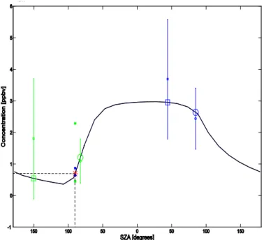
In this study, we use the box model to simulate diurnal ClO values for 1 km altitude steps from 35–45 km at the equator and during the day of equinox (spring, but this 15

is also the case for the autumn as well). Essentially, each ClO diurnal cycle can be expressed as a function of SZA, which in itself is a function of time. The purpose of doing this is so that the binned SMR profiles are scaled to a specific SZA, θ. This means for the equivalent satellite SZAθ_obsthe model values will yield a scale factorsf, which is then applied to the satellite measurement,

20

Y_scl(θ_mod,z)=Ymod(θmod,z)

Y_mod(θ_obs,z)

| {z }

sf

Y_obs(θ_obs,z) (2)

whereY_obsis the observed concentration profile,Y_modrepresents the model values,Y_scl is the scaled concentration profile, andz is the vertical coordinate. For this study we choseθ_mod₌90◦_{a.m. (i.e. morning). In order to make a fair comparison we also treat} the MLS data in the same manner, such that both data sets contain scaled vertical 25

(13)

ACPD

10, 8623–8655, 2010

A. Jones et al.

Title Page

Tables Figures

◭ ◮

Back Close

Full Screen / Esc

Interactive Discussion for whenθ_mod₌90◦_{a.m. More importantly it removes the LST problem concerning the}

SMR measurements and time of day no longer is a factor. A graphical illustration of the scaling process is given in Fig. 6.

When making a trend analysis the absolute values of the scaled monthly means are irrelevant as we only consider relative units by firstly removing the seasonal cycle 5

(similar to that of the HCl method). A linear regression analysis is made on each set of scaled deseasonalised anomalies although we do not fit for the solar cycle since the time series length of each data set is too short. Mean ClO changes due to 11-year solar forcing are typically 0–2% between 35 and 45 km (Egorova et al., 2005). Thus the remaining scaled anomalies will have the QBO and seasonal cycles removed, but 10

will still include the solar cycle contribution. Finally, a linear trend line is fitted to the all instrument average, which is calculated using the scaled SMR and MLS anomalies.

Finally, as a check, we have also analysed measurement scale factors based on other times of the year including the winter and summer solstices. It means that the observations are scaled differently owing to different conditions compared to those at 15

equinox. Such conditions are related to parameters like solar intensity (as a result of the alternating distance from the Earth to the Sun during an annual cycle) and variations in the maximum SZA during an annual cycle. However, we do not find any significant differences in the overall trend magnitudes using simulated diurnal cycles from the winter and summer solstice cases, therefore the choice of using a ClO diurnal cycle for 20

equinox is justified.

4 Results

4.1 HCl

Figure 7 shows the all instrument average for combined HALOE and ACE-FTS anoma-lies in the three bins analysed. Each bin shows an increase in HCl values monotonically 25

(14)

ACPD

10, 8623–8655, 2010

A. Jones et al.

Title Page

Tables Figures

◭ ◮

Back Close

Full Screen / Esc

Interactive Discussion typically 6–7% lower than the 1997 turn around anomaly estimates. After August 2004

ACE-FTS anomalies dominate the all instrument average. As ACE-FTS has a larger sampling rate compared to HALOE it means that the all instrument average is less noisy in comparison to the HALOE anomaly contribution.

We find that in each bin HCl values increase between ∼25.2%/decade and 5

33.2%/decade until 1997. In each case the trend magnitudes are statistically signif-icant from a zero trend at 2σ (or at a 95% confidence level). Error estimates are cal-culated using an algorithm suggested by Weatherhead et al. (1998). These estimates are comparable to those found by Newchurch et al. (2003), who examined HCl for the same altitude region using HALOE data from 1993–2003. Our estimates are though 10

larger, which could be a result of the “change in linear trend method”. Newchurch et al only apply a linear trend from 1993 until 1997, thus they only consider the anomalies during this time, while the change in linear trend method looks for a specific tempo-ral path through the whole data set. The di_fference being in this case that the for-mer method produces a less steep fit to the data in comparison to the latter method. 15

Trend values after 1997 all show consistent declines in HCl, where the largest magni-tude is found in the mid latimagni-tudes of−6.7%±2.4%/decade (Southern Hemisphere) and −6.4%±2.8%/decade (Northern Hemisphere). These values as well as the all instru-ment average for the tropics (−4.4%±2.0%/decade) are all statistically significant from a zero trend at 2σ.

20

4.2 ClO

A summary of the scaled SMR and MLS measurements is presented in Fig. 8. The upper panel illustrates AM and PM scaled monthly means for both SMR and MLS. It can be seen that there is an excellent agreement between the average SMR AM and PM scaled values. There is however about a 2–2.5 ppbv difference between MLS AM 25

(15)

ACPD

10, 8623–8655, 2010

A. Jones et al.

Title Page

Tables Figures

◭ ◮

Back Close

Full Screen / Esc

Interactive Discussion the scaling factors), yielding in this case unrealistically high scaled measurement

val-ues. The end result is a larger layer average. Due to this problem, we have decided to ignore the MLS night time measurements, thus we only consider MLS PM observations for the construction of the all instrument average. The bottom panel of Fig. 8 shows the SMR scaled monthly means (combination of a.m. and p.m.) as well as the MLS 5

PM scaled monthly means. There is a good agreement between the two scaled data sets, where each individual time series shows evidence for structural components due to natural variability, including the annual, SAO, and QBO cycles. Di_fferences between MLS and SMR are typically no larger than∼0.3 ppbv and there is also clear evidence that the LST trend in the SMR measurements is removed.

10

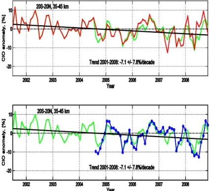
Examination of the ClO all instrument average based on the anomalies, with the sea-sonal and QBO cycles removed, is shown in Fig. 9. The top panel shows the SMR con-tribution to the all instrument average, while the bottom panel considers MLS. The trend calculated for the 2001–2008 period from both data sets is−7.1%±7.8%/decade, im-plying that it is not statistically significant from a zero trend at 2σ.

15

5 Discussion of HCl and ClO results

The ClO trend value obtained here is considerably lower, but consistent with the analy-sis done by Solomon et al. (2006), who used ground based millimetre wave measure-ments at Mauna Kea in Hawaii, USA, to observe ClO concentrations. They found a significant linear decline of ClO of−15%±2%/ decade from 1995–2005 for altitudes 20

between 35 and 39 km, although they estimate that about 30% of this decline can be attributed to methane (CH4) increments (a sink of Cl) in this altitude range, which have

been measured by HALOE. Our values are however consistent with the analysis by O’Doherty et al. (2004) who estimate that tropospheric Cly is decreasing between 6

and 8%/decade after the 1993 peak. We have also compared our ClO trend value with 25

(16)

anal-ACPD

10, 8623–8655, 2010

A. Jones et al.

Title Page

Tables Figures

◭ ◮

Back Close

Full Screen / Esc

Interactive Discussion ysed here (see the SPARC CCMVal “REF2” scenario described in Eyring et al. (2005)

for further details). The CMAM model estimates a trend of∼ −7%/decade since Jan-uary 2001 until the end of 2008, which is of similar magnitude with our calculated trend value.

Solomon et al. (2006) also investigated HALOE HCl between 35 and 39 km for 5

10◦N–30◦N. A fit to the HALOE data from 1997–2005 showed HCl to drop by −5%±1.2%/decade, which is in agreement with our findings of−4.4%±2.0%/decade at 30◦S–30◦N. This also suggests that since 2005 until present that HCl has continued to decrease at a similar rate. Simulated CMAM monthly averaged HCl values show that from 1997 to 2008, HCl decreases by∼ −3%/decade (for 35–45 km in the tropics), 10

which is slightly less than our estimated trend value. The di_fference in trend values can be attributed to differences in the choice of peak loading times of HCl assumed here and to that found in the CMAM model, where CMAM HCl peaks typically around 1999 and not 1997.

Linear trend model uncertainties are mainly determined by three factors (Weather-15

head et al., 1998; Reinsel et al., 2002): the time series length, the autocorrelation of the residuals, and variance of the residuals. In this analysis we find the ClO all instru-ment average anomalies to have an autocorrelation of 0.51, which is moderate (the degree of correlation increases towards 1 or−1), while the standard deviation is 4.4%. The ClO anomalies of course still have variations due to the solar cycle included, which 20

will account for some of the variance and autocorrelation in the modelled values. The variation of tropical ClO due to changes in solar intensity is estimated to be as much as 2% between 35 and 40 km, but it is almost negligible between 40 and 45 km according to model simulations (Egorova et al., 2005). The total length of the time series is also quite short, which means it is hard to differentiate between long and short term vari-25

(17)

ACPD

10, 8623–8655, 2010

A. Jones et al.

Title Page

Tables Figures

◭ ◮

Back Close

Full Screen / Esc

Interactive Discussion Ultimately, the apparent decline in chlorine compounds should mean an

anti-correlation with ozone. Recent ozone trends calculated for 1997 onwards in this altitude region have shown signs of a slow down of ozone depletion, although the magnitudes found are typically smaller than what are reported here. Jones et al. (2009) reported that ozone is increasing at∼1.7% (± ∼2.0%/decade) at mid-latitudes based on linear 5

trends from 1997–2008, while Steinbrecht et al. (2006) suggest a 1997–2005 trend for Hawaii to be increasing by 1.9%±1.9%/decade. Both of these examples show trend magnitudes to be less than the trend values estimated here using HCl and ClO. This implies that ozone’s recovery is also dependent on other atmospheric parameters and not just entirely on chlorine chemistry. For example, ozone is influenced by cycles in-10

volving, ClO, BrO, NO_x, and HO_x and thus depends on changes of the source gases of these families (such as H2O and CH4for the HOxfamily for example) (WMO, 2006).

6 Summary

During the last 17 years, HALOE and ACE-FTS together have provided measurements of HCl (1993 to 2008), while ClO has been observed by Aura-MLS and Odin/SMR for 15

a shorter period of time, 2001–2008. We have analysed long term changes of both of these gases by examining monthly averaged data in the 35–45 km altitude region for three latitude bands (60◦S–30◦S, 30◦S–30◦N, 30◦N–60◦N) for HCl measurements and 20◦S–20◦N for ClO.

We find that the SMR ascending and descending node LSTs are monotonically in-20

creasing in time since its launch. This has resulted in ClO measurements being signifi-cantly influenced by lower SZAs during morning scans and higher SZAs during evening scans. To remove the LST trend in the data we use a 1-D atmospheric box model to determine scale factors, which are applied to the measurements so that they will rep-resent a value when the SZA equals 90◦ during sunrise. We apply the same method 25

(18)

ACPD

10, 8623–8655, 2010

A. Jones et al.

Title Page

Tables Figures

◭ ◮

Back Close

Full Screen / Esc

Interactive Discussion 40 km. We chose not to implement the scaled MLS AM values in the trend analysis

and thus only consider MLS PM scaled values. SMR scaled values showed consis-tency between AM and PM profiles, thus both sets of scaled values are considered.

Anomalies of the monthly averages are calculated by removing the seasonal and QBO cycles. The anomalies are then concatenated in each respective bin to produce 5

all instrument averages, which are used for the trend analysis. We find that HCl shows post 1997 trends to be −4.4±2.0 %/decade (tropics),−6.4±2.8%/decade (northern mid-latitudes), and −6.7±2.4%/decade (southern mid-latitudes) in the upper strato-sphere. The modelling uncertainties indicate that the estimated trends are significantly different from a zero trend at 2σ. ClO trend estimates also show similar values since 10

2001 although, not statistically significant at 2σ(7.1±7.8%/decade). It is expected that in the future uncertainties of the ClO analysis will be reduced by employing a longer time series. It will also allow for the possibility to estimate the contribution of the solar cycle. This shows the importance of time series length. The fact that SMR has out lived its 2 year expected life time is a bonus as it has provided one of the longest ClO 15

data sets so far, hence it is important that the observations continue to be made until the satellite finally ceases to naturally operate.

The results found here are in agreement with and extend on previous findings (for example, Considine et al., 1997, 1999; Anderson et al., 2000; Newchurch et al., 2003; Froidevaux et al., 2006; Solomon et al., 2006; WMO, 2006) and illustrates that the 20

Montreal protocol and the subsequent amendments are having an impact on the total chlorine concentration in the stratosphere and ultimately the recovery of ozone.

Acknowledgements. Odin is a Swedish-led satellite project funded jointly by the Swedish Na-tional Space Board (SNSB), the European Space Agency (ESA), the Canadian Space Agency (CSA), the National Technology Agency of Finland (Tekes) and the Centre National d’Etudes 25

(19)

ACPD

10, 8623–8655, 2010

A. Jones et al.

Title Page

Tables Figures

◭ ◮

Back Close

Full Screen / Esc

Interactive Discussion would also like to thank the EU-SCOUT-O3 project and those involved for their contribution to

funding this work. Thanks also to Andreas Jonsson at the University of Toronto, Canada, for his help with the CMAM data.

References

Anderson, J., Russell III, J. M., Solomon, S., and Deaver, L. E.: Halogen Occultation Ex-5

periment confirmation of stratospheric chlorine decreases in accordance with the Montreal Protocol, J. Geophys. Res.,105, 4483–4490, 2000.

Beagley, S. R., de Grandpr ´e, J., Koshyk, J. N., McFarlane, N. J., and Shephard, T. G.: Radiative-dynamical climatological of he first-generation Canadian Middle Atmospheric Model, Atmos.-Ocean, 35, 293–331, 1997.

10

Bernath, P. F., McElroy, C. T., Abrams, M. C., Boone, C. D., Butler, M., Camy-Peyret, C., Car-leer, M., Clerbaux, C., Coheur, P.-F., Colin, R., DeCola, P., De Mazi `ere, M., Drummond, J. R.,Dufour, D., Evans, W. F. J., Fast, H., Fussen, D., Gilbert, K., Jennings, D. E., Llewellyn, E. J., Lowe, R. P., Mahieu, E., Mc-Connell, J. C., McHugh, M., McLeod, S. D., Michaud, R., Midwinter, C., Nassar, R., Nichitiu, F., Nowlan, C., Rinsland, C. P., Rochon, Y. J., Rowlands, 15

N., Semeniuk, K., Simon, P., Skelton, R., Sloan, J. J., Soucy, M.-A., Strong, K., Tremblay, P., Turnbull, D., Walker, K. A., Walkty, I., Wardle, D. A., Wehrle, V., Zander, R., and Zou, J.: Atmospheric Chemistry Experiment (ACE): Mission overview, Geophys. Res. Lett., 32, L15S01, doi:10.1029/2005GL022386, 2005.

Boone, C. D., Nassar, R.,Walker, K. A., Rochon, Y., McLeod, S. D., Rinsland, C. P., and Bernath, 20

P. F.: Retrievals for the Atmospheric Chemistry Experiment Fourier transform spectrometer, Appl. Optics, 44(33),7218–7231, 2005.

Bracher, A., Sinnhuber, M., Rozanov, A., and Burrows, J. P.: Using a photochemical model for the validation of NO₂satellite measurements at different solar zenith angles, Atmos. Chem. Phys., 5, 393–408, 2005,

25

http://www.atmos-chem-phys.net/5/393/2005/.

Brohede, S., McLinden, C. A., Berthet, G., Haley, C. S., Murtagh, D., and Sioris, C. E.: A stratospheric NO₂climatology from Odin/OSIRIS Limb-scatter measurements, Can. J. Phys, 85, 1253–1274, 2007a.

(20)

ACPD

10, 8623–8655, 2010

A. Jones et al.

Title Page

Tables Figures

◭ ◮

Back Close

Full Screen / Esc

Interactive Discussion Llewellyn, E. J., Bazureau, A., Goutail, F., Randall, C. E., Lumpe, J. D., Taha, G., Thomasson,

L. W., and Gordley, L. L: Validation of Odin/OSIRIS stratospheric NO₂profiles, J. Geophys. Res., 112, D07310, doi:10.1029/2006JD007586, 2007b.

Considine, G. D., Deaver, L., Remsberg, E. E., and Russell III, J. M.: HALOE Observations of a Slowdown in the Rate of Increase of HF in the Lower Mesosphere, Geophys. Res. Lett., 5

24(24), 3217–3220, 1997.

Considine, G. D., Deaver, L., Remsberg, E. E., and Russell III, J. M.: Analysis of Near- Global Trends and Variability in HALOE HF and HCl Data in the Middle Atmosphere, J. Geophys. Res., 104, 24297–24308, 1999.

Cunnold, D. M., Yang, E. S., Newchurch M. J., Reinsel G. C., Zawodny J. M., and Russell III, 10

J. M.: Comment on “Enhanced upper stratospheric ozone: Sign of recovery or solar cycle effect?”, by Steinbrecht et al., J. Geophys. Res., 109, D14305, doi:10.1029/2004JD004826, 2004.

de Grandpr ´e, J., Beagley, S. R., Fomichev,V. I., Gri_ffoen, E., McConnell, J. C., Medvedev, A. S., and Shepherd, T. G.: Results from the Canadian Middle Atmosphere Model, J. Geophys. 15

Res, 105, 26475–26491, 2000.

Egorova, T., Rozanov, E., Zubov, V., Schmutz, W., and Peter, Th.: Influence of solar 11-year variability on chemical composition of the stratosphere and mesosphere simulated with a chemistry-climate model, Adv. Space Res., 451–457, 2005.

Eyring, V., Kinnison, D. E., and Shepherd, T. G.: Overview of planned coupled chemistry-20

climate simulations to support upcoming ozone and climate assessments, SPARC Newslet-ter, 25, 11–17, 2005.

Frisk, U., Hagstrom, M., Ala-Laurinaho, J., Andersson, S., Berges, J. C., Chabaud, J. P., Dahlgren, M., Emrich, A., Floren, H. G., Florin, G., Fredrixon, M., Gaier, T., Haas, R., Hir-vonen, T., Hjalmarsson, A., Jakobsson, B., Jukkala, P., Kildal, P. S.,Kollberg, E., Lassing, 25

J., Lecacheux, A., Lehikoinen, P., Lehto, A., Mallat, J., Marty, C., Michet, D., Narbonne, J., Nexon, M., Olberg, M., Olofsson, A. O. H., Olofsson, G., Origne, A., Petersson, M., Piironen, P., Pons, R., Pouliquen, D., Ristorcelli, I., Rosolen, C., Rouaix, G., Raisanen, A. V., Serra, G., Sjoberg, F., Stenmark, L., Torchinsky, S., Tuovinen, J., Ullberg, C., Vinterhav, E., Wadefalk, N., Zirath, H., Zimmermann, P., and Zimmermann, R.: The Odin Satellite: I. Radiometer 30

Design and Test, Astron. Astrophys., 402, 27–34, 2003.

(21)

ACPD

10, 8623–8655, 2010

A. Jones et al.

Title Page

Tables Figures

◭ ◮

Back Close

Full Screen / Esc

Interactive Discussion J., Cunnold, D., and Waugh, D.: Temporal decrease in upper atmospheric chlorine, Geophys.

Res. Lett., 33, L23812, doi:10.1029/2006GL027600, 2006.

Froidevaux, L., Jiang, Y. B., Lambert, A., Livesey, N. J., Read, W. G., Waters, J. W., Fuller, R. A., Marcy, T. P., Popp, P. J., Gao, R. S., Fahey, D. W., Jucks, K. W., Stachnik, R. A., Toon, G. C., Christensen, L .E., Webster, C. R., Bernath, P .F., Boone, C. D., Walker, K .A., 5

Pumphrey, H. C., Harwood, R. S., Manney, G. L., Schwartz, M. J., Daffer, W. H., Drouin, B. J., Cofield, R. E., Cuddy, D. T., Jarnot, R. F., Knosp, B. W., Perun, V. S., Snyder, W. V., Stek, P. C., Thurstans, R. P., and Wagner, P. A.: Validation of Aura Microwave Limb Sounder HCl measurements, J. Geophys. Res., 113, D15S25, doi:10.1029/2007JD009025, 2008.

Jones, A., Urban, J., Murtagh, D. P., Eriksson, P., Brohede, S., Haley, C., Degenstein, D., 10

Bourassa, A., von Savigny, C., Sonkaew, T., Rozanov, A., Bovensmann, H., and Burrows, J.: Evolution of stratospheric ozone and water vapour time series studied with satellite mea-surements, Atmos. Chem. Phys., 9, 6055–6075, 2009,

Jonsson, A.: Modelling: the middle stratosphere and its sensitivity to climate change, Dept. of 15

Met. Stockholm University, PHD thesis, 2006.

Jucks, K. W., Johnson, D. G., Chance, K. V., Traub, W. A., Salawitch, R. J., and Stachnik, R. A.: Ozone production and loss rate measurements in the middle stratosphere, J. Geophys. Res., 101(D22), 28785–28792, 1996.

Mahieu, E., Duchatelet, P., Demoulin, P., Walker, K. A., Dupuy, E., Froidevaux, L., Randall, C., 20

Catoire, V., Strong, K., Boone, C. D., Bernath, P. F., Blavier, J.-F., Blumenstock, T., Coffey, M., De Mazi `ere, M., Griffith, D., Hannigan, J., Hase, F., Jones, N., Jucks, K. W., Kagawa, A., Kasai, Y., Mebarki, Y., Mikuteit, S., Nassar, R., Notholt, J., Rinsland, C. P., Robert, C., Schrems, O., Senten, C., Smale, D., Taylor, J., T ´etard, C., Toon, G. C., Warneke, T., Wood, S. W., Zander, R., and Servais, C.: Validation of ACE-FTS v2.2 measurements of HCl, HF, 25

CCl₃F and CCl₂F₂ using space-, balloon- and ground-based instrument observations, At-mos. Chem. Phys., 8, 6199–6221, 2008,

Molina, M. J. and Rowland, F. S.: Stratospheric sink for chlorofluoro-methanes: Chlorine atom catalysed destruction of ozone, Nature, 249, 810–812, 1974.

30

(22)

Mc-ACPD

10, 8623–8655, 2010

A. Jones et al.

Title Page

Tables Figures

◭ ◮

Back Close

Full Screen / Esc

Interactive Discussion Dade, I. C., Haley, C., Sioris, C., Savigny, C. von, Solheim, B. H., McConnell, J. C. , Strong,

K., Richardson, E. H., Leppelmeier, G. W., Kyr ¨ol ¨a, E., Auvinen, H., and Oikarinen L.: An overview of the Odin atmospheric mission, Can. J. Phys., 80, 309–319, 2002.

Newchurch, M. J., Yang, E. S., Cunnold, D. M., Reinsel, G. C., Zawodny, J. M., and Russel III, J. M.: Evidence for slowdown in stratospheric ozone loss: First stage of ozone recovery, J. 5

Geophys. Res., 108(D16), 4507, doi:10.1029/2003JD003471, 2003.

Newman, P. A., Daniel, J. S., Waugh, D. W., and Nash, E. R.: A new formulation of equivalent effective stratospheric chlorine (EESC), Atmos. Chem. Phys., 7, 4537–4552, 2007,

ODoherty, S., Cunnold, D. M., Manning, A., Miller, B. R., Wang, R. H. J., Krummel, P .B., 10

Fraser, P. J., Simmonds, P. G., McCulloch, A., Weiss, R. F., Salameh, P., Porter, L .W., Prinn, R. G., Huang, J., Sturrock, G., Ryall, D., Derwent, R. G., and Montzka S. A: Rapid growth of hydrofluorocarbon 134a and hydrochlorofluorocarbons 141b, 142b, and 22 from Advanced Global Atmospheric Gases Experiment (AGAGE) observations at Cape Grim, Tasmania, and Mace Head, Ireland, J. Geophys. Res., 109, D06310, doi:10.1029/2003JD004277, 2004. 15

Rinsland C. P., Mathieu, E., Zander R., et al.: Long-term trends of inorganic chlorine from ground-based infrared solar spectra: Past increases and evidence for stabilization J. Geo-phys. Res., 108(D8), 4252, doi:10.1029/2002JD003001, 2003.

Reinsel, G. C., Weatherhead, E. C., Tiao, G. C., Miller, A. J., Nagatani, R. M., Wuebbles, D. J., and Flynn, L. E.: On detection of turnaround and recovery in trend for ozone, J. Geophys. 20

Res., 107(D10), 4078, doi:10.1029/2001JD00500, 2002.

Russell III, J. M., Gordley, L. L., Park, J. H., Drayson, S. R. , Hesketh, D. H., Cicerone, R. J. , Tuck, A. F., Frederick, J. E., Harries, J. E., and Crutzen, P.: The Halogen Occultation Experiment, J. Geophys. Res., 98(D6), 10777–10797, 1993.

Russell, J. M., Deaver, L. E., Luo, M. Z., Park, J. H., Gordley, L. L., Tuck, A. F., Toon, G. 25

C., Gunson, M. R., Traub, W. A., Johnson, D. G., Jucks, K. W., Murray, D. G., Zander, R., Nolt, I. G., and Webster, C. R.: Validation of hydrogen chloride measurements made by the Halogen Occultation Experiment from the UARS platform, J. Geophys. Res., 101, 10151– 10162, 1996.

Santee, M. L., Lambert, A., Read, W. G., Livesey, N. J., Manney, G. L., Cofield, R. E., Cuddy, D. 30

(23)

ACPD

10, 8623–8655, 2010

A. Jones et al.

Title Page

Tables Figures

◭ ◮

Back Close

Full Screen / Esc

Interactive Discussion H., von Hobe, M., Toon, G. C., and Stachnik, R. A.: Validation of the Aura Microwave Limb

Sounder ClO Measurements, J. Geophys. Res., 113, D15S22, doi:10.1029/2007JD008762, 2008.

Schoeberl, M. R., Douglass, A. R., Polansky, B., Boone, C., Walker, K. A., and Bernath, P.: Estimation of stratospheric age spectrum from chemical tracers, J. Geophys. Res., 110, 5

D21303, doi:10.1029/2005JD006125, 2005.

Solomon, P., Barrett, J., Mooney, T., Connor, B., Parrish, A., and Siskind, D. E.: Rise and decline of active chlorine in the stratosphere, Geophys. Res. Lett., 33, L18807, doi:10.1029/2006GL027029, 2006.

Steinbrecht W., Claude, H., and Winkler P.: Enhanced stratospheric ozone: Sign of recovery or 10

solar cycle?, J. Geophys. Res., 109, D2308, doi:10.1029/2004JD004284, 2004.

Steinbrecht, W., Claude, H., Sch ¨onenborn, F., McDermid, I. S., Leblanc, T., Godin, S., Song, T., Swart, D. P. J., Meijer, Y. J., Bodeker, G. E., Connor, B. J., K ¨ampfer, N., Hocke, K., Calisesi, Y., Schneider, N., de la Noe, J., Parrish, A. D., Boyd, I. S., Bruhl, C., Steil, B., Giorgetta, M. A., Manzini, E., Thomason, L.W., Zawodny, J. M., McCormick, M. P., Russell III, J. M., 15

Bhartia, P. K., Stolarski, R. S., and Hollandsworth-Frith, S .M.: Long-term evolution of upper stratospheric ozone at selected stations of the Network for the Detection of Stratospheric Change (NDSC), J. Geophys. Res., 111, D10308, doi:10.1029/2005JD006454, 2006. Stiller, G. P., von Clarmann, T., H ¨opfner, M., Glatthor, N., Grabowski, U., Kellmann, S., Kleinert,

A., Linden, A., Milz, M., Reddmann, T., Steck, T., Fischer, H., Funke, B., L ´opez-Puertas, 20

M., and Engel, A.: Global distribution of mean age of stratospheric air from MIPAS SF₆ measurements, Atmos. Chem. Phys., 8, 677–695, 2008,

Urban, J., Lauti é, N., Le Flochmo ën, E., Jim énez, C., Eriksson, P., de La No ë, J., Dupuy, E., Ekstr öm, M., El Amraoui, L., Frisk, U., Murtagh, D., Olberg, M., Ricaud, P.: Odin/SMR limb 25

observations of stratospheric trace gases: Level 2 processing of ClO, N2O, HNO3, and O3 J. Geophys. Res., Vol. 110, No. D14, D14307, 10.1029/2004JD005741, 29, 2005.

Urban, J., Murtagh, D., Lauti é, N., Barret, B., de La No ë, J., Frisk, U., Jones, A., Le Flochmo ën, E., Olberg, M., Piccolo, C., Ricaud P., and R ösevall, J.: Odin/SMR limb observations of trace gases in the polar lower stratosphere during 2004–2005, Proc. ESA First Atmospheric 30

Science Conference, 8–12 May 2006, Frascati, Italy, edited by: Lacoste, H., ESA-SP-628 Noordwijk, European Space Agency, ISBN-92-9092-939-1, ISSN-1609-042X, 2006.

(24)

ACPD

10, 8623–8655, 2010

A. Jones et al.

Title Page

Tables Figures

◭ ◮

Back Close

Full Screen / Esc

Interactive Discussion Limb Sounder (EOS MLS) on the Aura satellite, IEEE Trans. Geosci. Remote Sens, 55,

1075–1092, 2006.

Waugh, D. W., Considine, D. B., and Fleming, E. L.: Is Upper Stratospheric Chlorine Decreasing as Expected?, Geophys. Res. Lett., 28(7), 1187–1190, 2001.

Weatherhead, E. C., Reinsel, G. C., Tiao, G. C., Meng, X-Li, Choi, D., Cheang, W. K., Keller, 5

T., DeLuisi, J., Weubbles, D. J., Kerr, J. B., Miller, A. J., Oltmans, S. J., and Frederick, J. E.: Factors affecting the detection of trends: Statistical considerations and applications to environmental data, J. Geophys. Res., 103(D14), 17149–17116, 1998.

World Meteorological Organisation (WMO): Scientfic Assessment of Ozone Depletion, 2006, Geneva, 2006.

(25)

ACPD

10, 8623–8655, 2010

A. Jones et al.

Title Page

Tables Figures

◭ ◮

Back Close

Full Screen / Esc

Interactive Discussion Fig. 1. Monthly averaged HCl measurements for HALOE (red) and ACE-FTS (blue) for 35–

(26)

ACPD

10, 8623–8655, 2010

A. Jones et al.

Title Page

Tables Figures

◭ ◮

Back Close

Full Screen / Esc

Interactive Discussion Fig. 2. Spatial coverage of the satellite instruments used. Blue squares indicate HALOE, and

(27)

ACPD

10, 8623–8655, 2010

A. Jones et al.

Title Page

Tables Figures

◭ ◮

Back Close

Full Screen / Esc

Interactive Discussion Fig. 3. HALOE (red line circle) and ACE-FTS (blue line dot) anomalies (for 30◦S–30◦N, 35–

(28)

ACPD

10, 8623–8655, 2010

A. Jones et al.

Title Page

Tables Figures

◭ ◮

Back Close

Full Screen / Esc

Interactive Discussion Fig. 4. Monthly averaged SMR ClO concentrations as a function of time (for binned profiles,

20◦_S–20◦_{N, 35–45 km), taken for ascending node scans. Middle, SMR LST (hour of day) as a}

(29)

ACPD

10, 8623–8655, 2010

A. Jones et al.

Title Page

Tables Figures

◭ ◮

Back Close

Full Screen / Esc

Interactive Discussion Fig. 5.Monthly averaged SMR ClO concentrations as a function of time anomalies (for binned

(30)

ACPD

10, 8623–8655, 2010

A. Jones et al.

Title Page

Tables Figures

◭ ◮

Back Close

Full Screen / Esc

Interactive Discussion (θ

(θ (θ , z), where θ

(θ

(31)

ACPD

10, 8623–8655, 2010

A. Jones et al.

Title Page

Tables Figures

◭ ◮

Back Close

Full Screen / Esc

Interactive Discussion Fig. 7. HCl anomalies for the all instrument average (green) produced from HALOE and

ACE-FTS monthly averaged data between 35 and 45 km. Top 30◦_N–60◦_{N. Middle, 30}◦_S–30◦_N.

(32)

ACPD

10, 8623–8655, 2010

A. Jones et al.

Title Page

Tables Figures

◭ ◮

Back Close

Full Screen / Esc

Interactive Discussion Fig. 8. Scaled SMR and MLS ClO observations as a function of time for 35–45 km and 20◦S–

(33)

ACPD

10, 8623–8655, 2010

A. Jones et al.

Title Page

Tables Figures

◭ ◮

Back Close

Full Screen / Esc

Interactive Discussion Fig. 9. ClO anomalies for SMR (red) and MLS (blue) for 20◦_S–20◦_{N and 35–45 km. Also}