www.atmos-chem-phys.net/11/5321/2011/ doi:10.5194/acp-11-5321-2011
© Author(s) 2011. CC Attribution 3.0 License.
Chemistry
and Physics
Analysis of HCl and ClO time series in the upper stratosphere using
satellite data sets
A. Jones1, J. Urban2, D. P. Murtagh2, C. Sanchez2, K. A. Walker1, N. J. Livesey3, L. Froidevaux3, and M. L. Santee3
1Department of Physics, University of Toronto, Toronto, ON, Canada
2Department of Earth and Space Science, Chalmers University of Technology, Gothenburg, Sweden 3Jet Propulsion Laboratory, California Institute of Technology, Pasadena, CA, USA
Received: 5 February 2010 – Published in Atmos. Chem. Phys. Discuss.: 6 April 2010 Revised: 28 April 2011 – Accepted: 18 May 2011 – Published: 9 June 2011
Abstract. Previous analyses of satellite and ground-based
measurements of hydrogen chloride (HCl) and chlorine monoxide (ClO) have suggested that total inorganic chlorine in the upper stratosphere is on the decline. We create HCl and ClO time series using satellite data sets extended to Novem-ber 2008, so that an update can be made on the long term evolution of these two species. We use the HALogen Oc-cultation Experiment (HALOE) and the Atmospheric Chem-istry Experiment Fourier Transform Spectrometer (ACE-FTS) data for the HCl analysis, and the Odin Sub-Millimetre Radiometer (SMR) and the Aura Microwave Limb Sounder (Aura-MLS) measurements for the study of ClO. Altitudes between 35 and 45 km and two mid-latitude bands: 30◦S– 50◦S and 30◦N–50◦N, for HCl, and 20◦S–20◦N for ClO and HCl are studied. ACE-FTS and HALOE HCl anomaly time series (with QBO and seasonal contributions removed) are combined to produce all instrument average time series, which show HCl to be reducing from peak 1997 values at a linear estimated rate of−5.1 % decade−1in the Northern Hemisphere and −5.2 % decade−1 in the Southern Hemi-sphere, while the tropics show a linear trend of−5.8 % per decade (although we do not remove the QBO contribution there due to sparse data). Trend values are significantly dif-ferent from a zero trend at the 2 sigma level. ClO is de-creasing in the tropics by −7.1 %±7.8 % decade−1 based on measurements made from December 2001 to November 2008. The statistically significant downward trend found in HCl after 1997 and the apparent downward ClO trend since 2001 (although not statistically significant) confirm how ef-fective the 1987 Montreal protocol objectives and its amend-ments have been in reducing the total amount of inorganic chlorine.
Correspondence to:A. Jones
1 Introduction
Stratospheric ozone depletion is the result of anthropogenic release of chlorofluorocarbons (CFCs) in the troposphere. The lifetimes of the CFCs in the troposphere are very long al-lowing for a build up of concentrations of these gases, which are slowly transported to the stratosphere. CFCs are even-tually photolysed in the stratosphere due to intense ultra vi-olet radiation, where active chlorine (Cl) is released and is available for the destruction of ozone (Molina and Rowland, 1974). However, due to the 1987 Montreal protocol agree-ment (and the subsequent adjustagree-ments), ozone depleting sub-stance (ODS) emissions have slowly been phased out. It has been estimated that the total inorganic loading of tropo-spheric Cl peaked in 1993 (Rinsland et al., 2003) and has decreased by ∼5 % through early 2002 (O’ Doherty et al., 2004). As it is estimated that it takes 3–6 years for air to be transported into the middle and upper stratosphere (Stiller et al., 2008), then peak stratospheric values are suggested to be somewhere between 1996 and 1999 (WMO, 2006). Based on assumptions that the international agreements are adhered to, it is proposed using the equivalent effective stratospheric chlorine (EESC) parameter that total Cl values will reach pre 1980 levels around 2040 (Newman et al., 2007).
This study intends to examine the long term evolution of HCl and ClO using satellite data sets of the Halogen Occulta-tion Experiment (HALOE), the Atmospheric Chemistry Ex-periment Fourier Transform Spectrometer (ACE-FTS), the Aura Microwave Limb Sounder (Aura-MLS), and the Odin Sub-Millimetre Radiometer (SMR). We examine altitudes from 35 to 45 km and mid-latitudes from 30◦S–50◦S and 30◦N–50◦N for HCl and 20◦N–20◦S for ClO and HCl. The choice for investigating this altitude region is because ClO and HCl together make up more than 95 % of the chlorine budget here (WMO, 2006). Additionally, it is in this altitude range where ozone is expected to show signs of a recovery first (Jucks et al., 1996). The analysis will make trend esti-mates based on monthly residual averaged data. By show-ing the current state of total inorganic chlorine in the strato-sphere, we can ascertain if the Montreal protocol objectives are still working.
2 HCl and ClO data sets
2.1 HALOE
The HALOE instrument aboard the Upper Atmosphere Research Satellite (UARS) was operational from Septem-ber 1991 to NovemSeptem-ber 2005. HALOE employed a solar oc-cultation instrument measuring many trace gases including HCl. Observations were made in the infrared part of the electromagnetic spectrum (between 2.45 and 10 µm) (Rus-sell et al., 1993). The HALOE occultation instrument was highly sensitive and obtained 15 occultation measurements during each sunrise/sunset by comparing the solar spectra to the spectra obtained whilst scanning through the atmo-sphere. This produced in essence a self calibrating instru-ment with long term stability. A vertical profile resolution of approximately 2–4 km was typically obtained for HCl, be-tween 10 and 65 km. Global coverage from about 80◦N and 80◦S was achieved in approximately six weeks. As solar occultation relies on the sun, it means there will be no mea-surements made during polar night in the winter hemisphere. Moreover, it should be noted that the coverage of HALOE degraded over time and there were fewer measurements dur-ing the later years of the mission. We suggest the reader to consult (http://haloe.gats-inc.com/home/index.php) for more details. For the trend analysis, we ignore data for 1991 and 1992 to stay consistent with the work done by Newchurch et al. (2003). The reason for their analysis not to include these two years was due to the fact that the slope of a linear fit will be greatly affected by the beginning and ending data values. Because the HALOE data start during the Pinatubo period, they were very cautious to obtain a robust regres-sion. Hence, they omitted any suspicious data. Data used in this analysis are from the HALOE v19 and can be ob-tained from http://haloe.gats-inc.com/home/index.php. The combined systematic and random uncertainties in the upper
stratosphere are typically between 12 and 15 %, while correl-ative measurements with other instrument data show agree-ment between 8 and 19 % (Russell et al., 1996).
2.2 ACE-FTS
Another infrared solar occultation instrument yielding ver-tical profiles of HCl concentrations is the ACE Fourier Transform Spectrometer (ACE-FTS) (Bernath et al., 2005). The SCISAT platform maintains a low Earth repeating orbit with a geographical coverage between approximately 85◦S– 85◦N, providing the opportunity for ACE-FTS to make
typ-ically 15 sunrise and 15 sunset solar occultations per day. Unlike HALOE, the ACE-FTS orbit does not change on a year to year basis, meaning that typically the same latitudes are sampled for a given time period.
Vertical profiles are retrieved from observed solar spectra using a non-linear least-squares global fit technique (Boone et al., 2005). Currently, HCl v2.2 VMRs are from ∼10– 50 km with a vertical resolution of approximately 3–4 km. Comparisons of ACE-FTS HCl to various other satellite and ground based instrumentation show that there is a good agreement of generally better than 5–10 % above 20 km (Mahieu et al., 2008). At present, no error analysis for ACE-FTS atmospheric products has been made. For this study, ACE-FTS v2.2 data are filtered according to various criteria: that the associated measurement uncertainty is not greater than 100 % of the corresponding VMR value. Data used in this analysis are the ACE-FTS measurements from February 2004–November 2008.
2.3 MLS
Stratospheric ClO is studied using measurements of the Mi-crowave Limb Sounder (Aura-MLS), which was launched in July 2004 on the NASA Aura satellite (from here on, we refer to Aura-MLS as MLS). This is the second MLS instrument, whereas the previous instrument, on board the UARS plat-form (hence, UARS MLS), operated for∼8 years between 1991 and 1999, but is not included in this analysis. MLS is a limb scanning instrument, observing thermal emission at millimetre and sub-millimetre wavelengths (Waters et al., 2006). MLS has the ability to measure at night and is not af-fected by stratospheric clouds. The Aura satellite maintains a suborbital track, covering 82◦S to 82◦N with an ascending
node of 13:45 h local solar time (LST) and makes approxi-mately 3500 scans per day.
satellite measurements (Santee et al., 2008). However, this is of little relevance here as we examine MLS ClO measure-ments between 6.5 and 1.6 hPa (∼35–45 km) where system-atic uncertainties are small.
MLS ClO data are screened using only profiles that have a zero status flag so that profiles with possible ambiguities are removed. Data are also only used if the quality flag is greater than 0.8. Moreover, we reject values that have a poor conver-gence criterion such that it is larger than 1.5. Finally, values that possess a negatively flagged uncertainty (precision) are also rejected. Please see Santee et al. (2008) for more details.
2.4 Odin/SMR
The Odin satellite was launched in the beginning of 2001 and is a joint initiative between Sweden, Canada, Finland and France. This small satellite comprises two instruments, the Sub-Millimetre Radiometer (SMR) and the Optical Spectro-graph InfraRed Imager System (OSIRIS). The Odin satellite is polar orbiting (82.5◦S to 82.5◦N) and is sun synchronous with a descending node at 06:00 h and ascending node at 18:00 h LST. The SMR instrument makes measurements of various species including stratospheric ClO by observing thermal emission in the microwave region during day and night (Murtagh et al., 2002; Frisk et al., 2003). SMR con-sists of five receivers, where we use ClO from the 501.8 GHz band. We remove profiles if the quality flag is not equal to zero or for any observation with a measurement response less than 0.75.
The newest version of SMR, data version 2.1 (produced at the Chalmers University of Technology, Sweden), is used for the analysis of stratospheric ClO. The study by Santee et al. (2008) compares coincident MLS and SMR measure-ments, and it is found that there is an excellent agreement for altitudes between 35 and 45 km (within 0.1 ppbv). An overview of the SMR ClO measurements can be found in Urban et al. (2005, 2006). Note that SMR v2.1 and v2.0 ClO products are virtually identical. The vertical resolution for the ClO product at 501.8 GHz is 2–4 km in the stratosphere.
3 Methodology
Here, we describe the methods used in order to derive long term trends of stratospheric HCl and ClO. We use separate methodologies for each species, although a linear regression analysis is used in each case to derive the resulting trends.
3.1 HCl
As the main focus of the HCl analysis is on the upper strato-sphere, we firstly filter both HALOE and ACE-FTS data be-tween 35 and 45 km into three latitude bands: 30◦S–50◦S, 20◦S–20◦N, and 30◦N–50◦N. Monthly averages are calcu-lated for the filtered data. Each data set comprises a large
1993 1995 1997 1999 2001 2003 2005 2007 2.2
2.4 2.6 2.8 3
VMR [ppbv]
1993 1995 1997 1999 2001 2003 2005 2007 2.2
2.4 2.6 2.8 3
VMR [ppbv]
1993 1995 1997 1999 2001 2003 2005 2007 2.2
2.4 2.6 2.8 3
Year
VMR [ppbv]
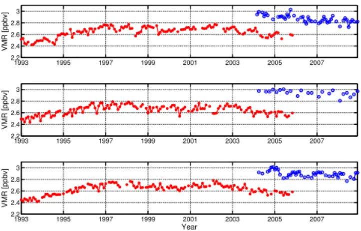
Fig. 1.Monthly averaged HCl measurements for HALOE (red) and ACE-FTS (blue) for 35–45 km in three latitude bands. Top, 30◦N– 50◦N. Middle, 20◦S–20◦N. Bottom, 30◦S–50◦S.
>300–500 profiles a month). A typical example of spatial coverage for all four instruments studied in this analysis is illustrated in Fig. 2. Here, the HALOE and ACE-FTS or-bital paths represent the typical spatial coverage completed during one month, while the SMR and MLS orbital paths are the typical spatial coverage for observations made during one day.
3.1.1 Removing known sources of variation
The variations of each individual time series are cyclic in nature and are associated mainly to seasonal cycles (includ-ing SAO) and the quasi-biennial oscillation (QBO). HCl’s response to variations in solar intensity are small between 35 and 45 km (Egorova et al., 2005) and is not accounted for in this analysis. By being able to separate the relative contributions of known variation (by the process of linear re-gression), we will be left with the unexplained variability of the monthly mean signal to which a linear trend can be ap-plied. We follow similar approaches to that of Newchurch et al. (2003), and Steinbrecht et al. (2004, 2006), where we firstly remove the seasonal cycle from the HCl time series. This is simply done for each instrument by finding the dif-ference between each monthly mean value from their corre-sponding average (climatological) annual cycle. For exam-ple, the HALOE mean January value calculated for all Jan-uarys during 1993–2005 is subtracted from each individual HALOE January VMR value. Hence, the resulting HALOE and ACE-FTS time series will be a monthly mean HCl time series with the seasonal components removed, but still con-taining contributions from the QBO and other sources of variation.
In order to model the HCl anomalies from HALOE and ACE-FTS time series (with the seasonal component already removed), we apply a linear regression model to each set of anomalies independently, accounting for fluctuations related to the QBO
Fig. 2. Spatial coverage of the satellite instruments used. Blue squares indicate HALOE, magenta diamonds indicate ACE-FTS, red stars indicate Odin-SMR, and green circles indicate MLS. HALOE and ACE-FTS measurements are for the month of January 2005. MLS and SMR observations are for the 1 January 2005.
[1HCl]t=b+at+
QBO
X
i=1
cicos
2π t PQBO(i)
+disin
2π t PQBO(i)
+Nt,(1)
where1HCl(t )are the HCl anomalies calculated for each month,t. The first and second components in the model rep-resent a linear trend, whereb is a constant when timet=0 anda is a linear fit coefficient. The third set of terms rep-resents the QBO cycle, which is a combination of cosine and sine wave functions, which use harmonics, PQBO(i), that best represent the behaviour of the QBO cycle. The last term in the model, Nt, is the residual or autocorrelated error term, which is an autoregressive process such that, Nt=θ Nt−1+et, whereθis the autocorrelation (lag 1 month) andet are the white noise residuals with zero mean and com-mon variance. As we have already removed the seasonal cy-cle prior to this step, there is no need to include a seasonal cycle component. We have chosen to do this as we treat the tropical bin slightly different since we do not fit for the QBO parameter. The reason for this is due to the sparse contri-bution of ACE-FTS HCl data between 20◦S–20◦N, which
causes difficulties in estimating reliable harmonics represent-ing the cyclic behaviour of the QBO.
The termsa,b,candd need to be calculated so that the total summed contribution of the QBO can be determined. Hence, Eq. (1) can be solved for pre-determined QBO cy-cles (PQBO(i))by least squares analysis such that the sum of the squares of the residuals is minimised. Thus, the remain-ing HCl monthly anomalies are from sources of variabil-ity that cannot be explained by seasonal or QBO behaviour. The fundamental period of the QBO in the tropics is around 30 months, but there are also smaller periods modulating around 12 months, especially relevant for the mid-latitudes (Baldwin et al., 2001). Furthermore, Steinbrecht at al. (2004) showed statistically significant (at 90 %) periods found in ground-based stratospheric ozone data, to be between 7.5 and 32.2 months. Here, we estimate the QBO signals by examining the HCl deseasonalised time series directly, when passed through a fast Fourier transform (FFT). Large peaks observed between 7–9, 16–22, and 26–32 months in the re-sulting FFT power spectrum give an estimate to those cycles that are due to the QBO and are used asPQBO(i)in the regres-sion model. We then compare the summed QBO component to zonal wind data provided at 10 hPa over Singapore to en-sure that the modeled QBO component has the correct degree of phasing, such that there will be a phase shift in the mod-eled QBO output due to the delay in the transport of air from the tropics (typically 6–18 months Stiller et al., 2008).
3.1.2 Applying a trend to anomaly time series after
seasonal and QBO components are removed
Examination of the HALOE anomalies (with the season and QBO contributions removed) for the southern mid-latitude bin in Fig. 3, shows little difference in structure for the same bin to that exhibited in Fig. 1. The Northern Hemi-sphere mid-latitude and tropics bin show similar structures, (not shown here), hence we assume that the turnaround time for HCl to be 1997 for both bins, which also agrees with EESC peak times in this altitude range (Newman et al., 2007; WMO, 2006; Schoeberl et al., 2005). In order to quantify the HALOE anomalies, we would like to try and estimate a lin-ear trend before and after 1997. This can be done by apply-ing the change in linear trend method suggested by Reinsel et al. (2002). Here, a piece-wise linear trend is defined over the total time series period,T, such that there is a change in trend magnitude at a given time,t=T0and is described here as
[1HALOEHCl]t=b+a1X1t+a2X2t+Nt, (2) where1HALOEHCl(t )are the HALOE HCl anomalies to be modeled with seasonal and QBO parameters removed.Xt is a linear trend function,bis the intercept att=0, whilea1is the trend at timet=0, anda2signifies the magnitude of a possible change in trend at timet=T0. Thus
X1t=twhere 0< t≤T X2t=
0 0< t≤T0 (t−T0) T0< t≤T
.
1993 1995 1997 1999 2001 2003 2005 2007 -15
-10 -5 0 5 10
Year
HCl Residuals [%]
Fig. 3. HALOE (red line circle) and ACE-FTS anomalies (orange dot line) for 30◦S–50◦S, 35–45 km after seasonal and QBO terms are removed. ACE-FTS anomalies are shifted so that they align with the HALOE values (blue dot line). The solid black line indicates the fit line of HALOE extrapolated beyond 2005. The dashed line indicates the turn around year for HALOE HCl values (1997). The green star indicates the mean value along the HALOE fit line during the overlapping period with ACE-FTS. The value at the star is the offset value, which is applied to the ACE-FTS anomalies so that they shift relative to the HALOE anomalies for the overlapping time period.
Hence, Eq. (2) can be simplified to
anomalies are offset by−1.15 % (as indicated by the green star in Fig. 3). It should be noted that due to the measure-ment noise and the natural variability of the atmosphere there will be a residual offset uncertainty, which contributes to the overall correlated error term in the trend uncertainty.
When the ACE-FTS anomaly time series is aligned cor-rectly with the HALOE anomalies, we can then create an all instrument average where both instrument anomaly time series are combined and averaged. Hence, where there is data overlap between ACE-FTS and HALOE an average of the two is calculated. Due to the influence of the ACE-FTS anomalies in the all instrument average, it means that the original estimated trends calculated only for the HALOE time series using Eq. (2) will now need updating. Hence, we make new trend calculations based on the all instrument av-erage produced in each bin,1All instHCl(t ), before and after 1997 using Eq. (2).
3.2 ClO
Similarly to the HCl analysis, we have decided to investi-gate ClO in the upper stratosphere, from 35 to 45 km, but only for the tropics between 20◦S to 20◦N. As MLS makes retrievals on pressure surfaces, we filter data by using ap-proximate pressure surfaces that closely match the geomet-ric altitude zones used here: 6.4–1.6 hPa∼35–45 km. As ClO has a strong diurnal variation, it is important to con-sider the local solar time (LST) of the measurements of both SMR and MLS. As SMR has an ascending node around 06:00 h and descending node around 18:00 h, we expect the satellite to pass between 20◦S to 20◦N somewhere between
05:00–07:00 h and 17:00-19:00 h. A similar principle applies to MLS, which observes ClO in the ascending node from 12:45–14:45 h and descending node from 00:45-02:45 h for this latitude range. Hence, data must be also filtered accord-ing to time of day.
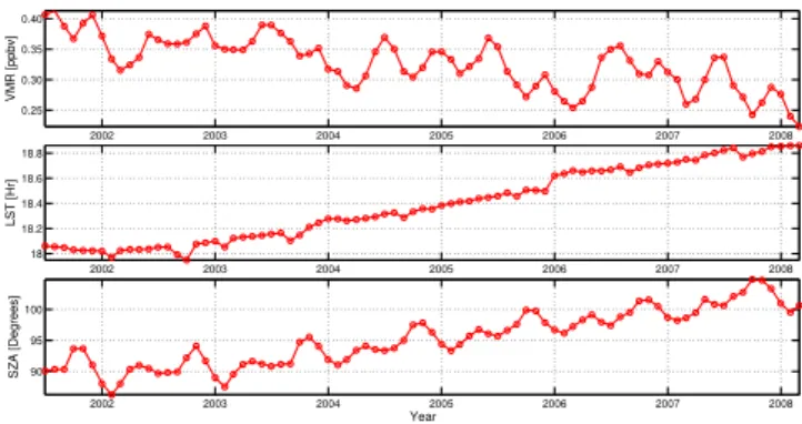
On examination of the SMR measurements, it was found that the ascending and descending node LSTs have been slowly drifting forwards since Odin’s launch. The reason for this is because the Odin satellite has slowly descended from its initial position during its mission. Figures 4 and 5 illus-trate the effect that this has on the monthly averaged ClO measurements for both dawn and dusk, illustrating the as-cending and desas-cending nodes respectively. As a result of in-creasing LST, it also means that the solar zenith angle (SZA) has slowly decreased over time during morning scans and increased during evening scans. The overall concentrations observed by SMR have therefore slowly increased (morning) or decreased (evening) over time. This causes problems if a trend analysis is to be made using the SMR data set as the induced trend in the measurements from the increased LST will be the dominating feature. For the record, we do not see such problems using MLS for either day or night time measurements since the Aura satellite has orbit stabilization.
2002 2003 2004 2005 2006 2007 2008
0.10 0.15 0.20 0.25
VMR [ppbv]
2002 2003 2004 2005 2006 2007 2008
6.2 6.4 6.6 6.8
LST [Hr]
2002 2003 2004 2005 2006 2007 2008
75 80 85 90
Year
SZA [Degrees]
Fig. 4. Monthly averaged SMR ClO concentrations as a function of time (for binned profiles, 20◦S–20◦N, 35–45 km), taken for ascending node scans. Middle, SMR LST as a function of time. Lower, SMR SZA as a function of time.
2002 2003 2004 2005 2006 2007 2008
0.25 0.30 0.35 0.40
VMR [ppbv]
2002 2003 2004 2005 2006 2007 2008
18 18.2 18.4 18.6 18.8
LST [Hr]
2002 2003 2004 2005 2006 2007 2008
90 95 100
SZA [Degrees]
Year
Fig. 5.Same as Fig. 4, except results are for descending node scans.
the modelling of the HALOE gases are reduced. Moreover, by modelling the same day consecutively 15 times or longer ensures that all the chemical abundances in the model con-verge, such that subsequent model runs produce insignificant changes for all modeled species.
In this study, we use the box model to simulate diurnal ClO values for 1 km altitude steps from 35–45 km at the equator and during the day of equinox (spring, autumn would pro-duce the same results). Essentially, each ClO diurnal cycle can be expressed as a function of SZA, which in itself is a function of time. The purpose of doing this is to calculate scaling factors, allowing for the binned SMR profiles to be scaled to a specific SZA,θ. This means for the equivalent satellite SZA,θobs, the model values will yield a scale factor,
sf, which is then applied to the satellite measurement, Yscl(θmod,z)=
Ymod(θmod,z) Ymod(θobs,z)
| {z }
sf
Yobs(θobs,z) (4)
whereYobsis the observed concentration profile,Ymod repre-sents the model values,Ysclis the scaled concentration pro-file, andzis the vertical coordinate. For this study we chose θmod=90◦am (i.e. morning). In order to make a fair com-parison, we also treat the MLS data in the same manner, such that both data sets contain profiles corrected for diur-nal variation (according to Eq. 4) from 35 to 45 km that can be used to produce monthly means based solely for when θmod=90◦am. More importantly, it removes the LST
prob-lem concerning the SMR measurements and time of day no longer is an issue. A graphical illustration of the scaling pro-cess is given in Fig. 6.
When making a trend analysis the absolute values of the scaled monthly means are irrelevant as we only consider rel-ative units by firstly removing the seasonal cycle (similar to that of the HCl method). A linear regression analysis is made (according to Eq. 1) on each set of scaled deseasonalised anomalies. We do not fit for the solar cycle since the time series length of each data set is too short. Mean ClO changes due to 11-year solar forcing are typically 0–2 % between 35 and 45 km (Egorova et al., 2005). Thus the remaining scaled anomalies will have the QBO and seasonal cycles removed, but will still include the solar cycle contribution. We apply an offset to the MLS anomalies so that they fit relative to the SMR anomalies. An all instrument average is created by combining the overlapping MLS (after applied offset) and SMR anomalies. Finally, a linear trend line is fitted to the all instrument average.
For reference, we have also analysed measurement scale factors based on other times of the year, including the win-ter and summer solstices. It means that the observations are scaled differently owing to different conditions compared to those at equinox. Such conditions are related to parameters like solar intensity (as a result of the alternating distance from the Earth to the Sun during an annual cycle) and variations in
150 100 50 0 50 100 150 -0.1
0 0.1 0.2 0.3 0.4 0.5 0.6
SZA [Degrees]
VMR [ppbv]
Fig. 6. An illustration of how the scale factors are calculated from Eq. (4) for measurements at z=40 km. ClO diurnal cy-cle (black line) as a function of time (SZA). Satellite observations
Yobs(θobs,z) are symbolized by either an open small circle (SMR) or an open small square (MLS). The observations are colour coded such that green = AM observations and blue = PM observations. The vertical solid lines are the corresponding measurement uncertain-ties. The large open circles correspond toYmod(θobs,z). The red asterisk is theYmod(θmod,z), whereθmod=90◦am. The resulting scaled measurementsYscl(θmod,z) are shown as small filled circles (SMR) or squares (MLS). Corresponding scaled measurement un-certainties are not shown.
the maximum SZA during an annual cycle. However, we do not find any significant differences in the overall trend mag-nitudes using simulated diurnal cycles from the winter and summer solstice cases, therefore the choice of using a ClO diurnal cycle for equinox is justified.
4 Results
4.1 HCl
Figure 7 shows the all instrument average for combined HALOE and ACE-FTS anomalies in the three bins analysed. Each bin shows an increase in HCl values monotonically un-til around 1997. Values slowly start to decrease after 1997 and by mid 2008 they are typically 5–6 % lower than the 1997 turn around anomaly estimates.
1993 1995 1997 1999 2001 2003 2005 2007 -15
-10 -5 0 5 10
HCl anomalies [%]
1993 1995 1997 1999 2001 2003 2005 2007
-15 -10 -5 0 5 10
HCl anomalies [%]
1993 1995 1997 1999 2001 2003 2005 2007
-15 -10 -5 0 5 10
Year
HCl anomalies [%]
1993 -1996 Trend = 32.4 +/- 1.7 %/decade 1993 -1996 Trend = 27.0 +/- 1.6 %/decade
1997 - Present Trend = -5.1 +/- 2.1 %/decade
1997 - Present Trend = -5.8 +/- 1.7 %/decade
1997 - Present Trend = -5.2 +/- 2.2 %/decade 1993 -1996 Trend = 25.0 +/- 1.4 %/decade
Fig. 7. HCl anomalies for the all instrument average (green) pro-duced from HALOE and ACE-FTS monthly averaged data between 35 and 45 km. Top 30◦N–50◦N. Middle, 20◦S–20◦N. Bottom, 30◦S–50◦S. The vertical black dot-dash line at 1997 indicates the turnaround date. The solid black lines indicate the fitted trend to the all instrument average before and after 1997. Trend values are given in % decade−1and uncertainties are 2 standard deviations. Please note that the 20◦S–20◦N contains a QBO contribution, while the extra tropical bins have the QBO removed.
result of the “change in linear trend method”. Newchurch et al. (2003) only apply a linear trend from 1993 until 1997, thus they only consider the anomalies during this time, while the change in linear trend method looks for a specific tem-poral path through the whole data set. The difference being in this case that the method used here produces a less steep fit to the data in comparison to the Newchurch et al. (2003) method. Trend values after 1997 all show consistent de-clines in HCl:−5.2 %±2.2 % decade−1in the southern mid-latitudes and−5.1 %±2.1 % decade−1in the northern hemi-spheric mid-latitudes. These values are all statistically signif-icant from a zero trend at 2σ. It is also seen that the sudden increase in values after 2001 (most apparent in 30◦S–50◦S) reported in Fig. 1 is still present, implying that according to this analysis it is neither a related feature of seasonal or QBO behaviour. This feature may be related to possible anomalous atmospheric dynamics in the Southern Hemisphere, such as the Antarctic ozone hole split in 2002 (Manney et al., 2005; Charlton et al., 2005) and/or changes in tropical upwelling due to enhanced wave driving in 2000–2001 (Dhomse et al., 2008). The tropics bin from 20◦S–20◦N shows a more neg-ative trend of 5.8 % decade−1 since 1997 compared to the mid-latitudes. However, we have not removed the QBO con-tribution from HALOE or ACE time series, suggesting the calculated trend could be different if the QBO contribution is removed.
4.2 ClO
A summary of the scaled SMR and MLS measurements is presented in Fig. 8. The upper panel illustrates AM and PM scaled monthly means for both SMR and MLS. It can be seen that there is an excellent agreement between the aver-age SMR AM and PM scaled values. There is however about a 0.1–0.2 ppbv difference between MLS AM and PM scaled values. The MLS AM measurements are made typically when the LST is between 01:00 h and 03:00 h, a time when ClO concentrations are close to zero ppbv below 40 km. As a result, small systematic errors of the measurements may be amplified by the diurnal correction factors, yielding in this case unrealistically high scaled measurement values. The end result is a larger layer average. Due to this problem, we have decided to ignore the MLS night time measurements, thus we only consider MLS PM observations for the con-struction of the all instrument average (note, that the offset is applied to the MLS PM anomalies so that they fit rela-tive to the SMR PM anomalies). The bottom panel of Fig. 8 shows the SMR scaled monthly means (combination of AM and PM) as well as the MLS PM scaled monthly means. There is a good agreement between the two scaled data sets, where each individual time series shows evidence for struc-tural components due to nastruc-tural variability, including the sea-sonal and QBO cycles. Differences between MLS and SMR are typically no larger than∼0.03 ppbv and there is also clear evidence that the LST trend in the SMR measurements is re-moved.
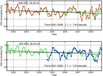
Examination of the ClO all instrument average based on the anomalies, with the seasonal and QBO cycles re-moved, is shown in Fig. 9. The top panel shows the SMR contribution to the all instrument average, while the bot-tom panel considers MLS. The trend calculated for the 2001–2008 period from both the combined data sets is
−7.1 %±7.8 % decade−1, implying that it is not statistically significant from a zero trend at 2σ.
5 Discussion of HCl and ClO results
The ClO trend value obtained here is considerably less nega-tive than the analysis performed by Solomon et al. (2006), who used ground based millimetre wave measurements at Mauna Kea in Hawaii, USA, to observe ClO concentra-tions. They found a significant linear decline of ClO of
−15 %±2 %/ decade from 1995–2005 for altitudes between 35 and 39 km, although they estimate that about 30 % of this decline can be attributed to methane (CH4)increments (a sink of Cl) in this altitude range, which have been mea-sured by HALOE. A recent update of this analysis, where the time series was extended to 2007, shows a ClO trend of
2002 2004 2006 2008 0.08
0.10 0.12 0.14 0.16
ClO VMR [ppbv]
Year
2002 2004 2006 2008
0.05 0.10 0.15 0.20 0.25 0.30
ClO VMR [ppbv]
Year
Fig. 8. Scaled SMR and MLS ClO observations as a function of time for 35–45 km and 20◦S–20◦N. Top, AM and PM scaled monthly averages; MLS AM blue star, MLS PM blue dot, SMR dawn red solid line, SMR dusk red dash line. Bottom, SMR (red) scaled combined AM and PM profiles, and MLS scaled (blue) day profiles.
2002 2003 2004 2005 2006 2007 2008
-20 -10 0 10
ClO anomalies [%]
Year
2002 2003 2004 2005 2006 2007 2008
-20 -10 0 10
ClO anomalies [%]
Year 20S-20N, 35-45 km
20S-20N, 35-45 km
Trend 2001-2008: -7.1 +/- 7.8%/decade
Trend 2001-2008: -7.1 +/- 7.8%/decade
Fig. 9. ClO anomalies for SMR (red) and MLS (blue) for 20◦S– 20◦N and 35–45 km. Also shown under-laid is the all instrument average (green). The solid black line shows the linear trend fitted to the all instrument average. Trend value given in % decade−1and uncertainties are at 2 standard deviations.
8 % decade−1. We have also compared our ClO trend value with results from the Canadian Middle Atmospheric Model (CMAM) (Beagley et al., 1997; de Grandpr´e et al., 2000) for the same time period, altitude layer, and latitudes bins used here (see the SPARC CCMVal “REF2” scenario described in Eyring et al. (2005) for further details). The CMAM model estimates a trend of∼ −7 % decade−1 since January 2001 until the end of 2008, which is of similar magnitude with our calculated trend value.
Table 1. HALOE trend and uncertainty (2σ) estimates before and after 1997.
Bin Trend before 1997 Trend after 1997
30◦S to 25◦S 28±1.4 % decade−1 −5.2±1.9 % decade−1
25◦S to 20◦S 30±1.4 % decade−1 −6.0±2.0 % decade−1
20◦S to 15◦S 26.7±1.6 % decade−1 −5.6±1.8 % decade−1
15◦S to 10◦S 23.8±1.5 % decade−1 −5.6±1.5 % decade−1
10◦S to 5◦S 21.4±1.6 % decade−1 −5.3±2.0 % decade−1
5◦S to 0◦ 24.3±2.1 % decade−1 −5.7±2.7 % decade−1
0◦to 5◦N 16.9±1.8 % decade−1 −4.2±2.2 % decade−1
5◦N to 10◦N 23.8±1.5 % decade−1 −4.1±1.9 % decade−1
10◦N to 15◦N 21.7±1.5 % decade−1 −4.6±1.9 % decade−1
15◦N to 20◦N 26.1±1.5 % decade−1 −5.5±1.9 % decade−1
20◦N to 25◦N 25.7±1.5 % decade−1 −5.3±1.9 % decade−1
25◦N to 30◦N 23.1±1.4 % decade−1 −4.5±1.7 % decade−1
10◦S to 10◦N 22.5±1.7 % decade−1 −5.3±2.1 % decade−1
15◦S to 15◦N 23.2±1.5 % decade−1 −5.4±1.9 % decade−1
20◦S to 20◦N 24.7±1.4 % decade−1 −5.7±1.8 % decade−1
30◦S to 30◦N 26.6±1.4 % decade−1 −5.7±1.4 % decade−1
Newchurch et al. (2003) examined HALOE observations from 30◦S–30◦N, but as HALOE had a sparse coverage due to the temporal progression of the scans as the satellite or-bited from pole to pole, it means the total global coverage varied strongly from year-to-year. This implies that a bin covering a 60◦ span over the tropical zone is perhaps too large and there will be strong influences from different chem-ical and dynamchem-ical regimes. In order to test how the HALOE HCl behaves in the tropics, we have examined HALOE resid-uals in 5◦latitude bands spanning 30◦S–30◦N. The HALOE
residuals examined have only the seasonal component re-moved. As there is a sparse amount of data in each five de-gree bin, estimating a QBO component could be challenging, hence the QBO component is retained in the residuals. Using the analogy of Eq. (2), we apply the Reinsel et al. (2002) fit-ting technique to the HALOE residuals from January 1993 to November 2005 with a turnaround of January 1997. Table 1 shows the estimated trends before and after the turnaround date for the five degree latitude bins and four extra larger bins for a fuller comparison: 10◦S–10◦N, 15◦S–15◦N, 20◦S– 20◦N, and 30◦S–30◦N.
from a peak and decline in CFC concentrations after 1997. Examination of the trends for the four larger bins (10◦S–
10◦N, 15◦S–15◦N, 20◦S–20◦N, and 30◦S–30◦N) shows
that the differences in trend magnitude between each bin is relatively small, indicating that the use of larger bins is acceptable, although caution is needed. We chose to use 20◦S–20◦N for representing the tropics in Fig. 7 so as to stay consistent with the ClO analysis. It should be noted that the trends for 20◦S–20◦N in Fig. 7 are slightly different to those in Table 1. This is simply because the ACE-FTS data has now been added to the all instrument average, which al-ters the time series properties when the Reinsel fit is made. The all instrument average for the tropics (and the tropical trend estimates from Table 1) are not dissimilar from the mid-latitude all instrument average trends shown in Fig. 7, although the QBO contributions are removed from the mid-latitude calculations and not for the tropics. It suggests that since 2005 until present, HCl has continued to decrease at a similar rate. Solomon et al. (2006) also investigated HALOE HCl between 35 and 39 km for 10◦N–30◦N, where they ap-plied a fit to the HALOE data from 1997–2005, producing a HCl linear trend of−5 %±1.2 % decade−1, which is simi-lar to the all instrument average values found in this study as well as the HALOE values from Table 1. Simulated CMAM monthly averaged HCl values show that from 1997 to 2008 HCl decreases by−3.1 % decade−1, for 35–45 km at north-ern mid-latitudes and−4.1 % decade−1 at Southern Hemi-sphere mid-latitudes, values which are slightly less than our estimated trend values. The difference in trend values can be attributed to differences in the choice of peak loading times of HCl assumed here and to that found in the CMAM model, where CMAM HCl peaks typically around 1999 and not 1997. Recent trend analyses concerning the upper strato-sphere (∼55 km) have been performed, using various satel-lite and ground-based data. Aura-MLS and ACE-FTS trend values show a decline in HCl to be −6 %±1 % decade−1 and−9 %±2 % decade−1respectively, since 2004. More-over, ground-based FTIR total column measurements of HCl at Jungfraujoch and Kiruna show similar trends from 1996– 2009: −9 %±1 % decade−1 and−8 %±2 % decade−1 re-spectively (WMO, 2011). These reported trends are larger in magnitude compared to here. However these differences can be possibly explained due to contrasts in HCl abundances with respect to altitude. HCl is estimated to account for >95 % of the total chlorine above 50 km compared to∼80– 90 % between 35 and 45 km (WMO, 2006). Moreover, there are different chemical and dynamical processes controlling the evolution of HCl throughout the stratosphere, hence we do not necessarily expect to see similar trend magnitudes.
Linear trend model uncertainties are mainly determined by three factors: the time series length, the autocorrelation of the residuals, and variance of the residuals factors (Weatherhead et al., 1998; Reinsel et al., 2002). In this analysis, we find the ClO all instrument average anomalies to have an autocorre-lation of 0.51, which is moderate (the degree of correautocorre-lation
increases towards 1 or−1), while the standard deviation is 4.4 %. The ClO anomalies of course still have variations due to the solar cycle included, which will account for some of the variance and autocorrelation in the modeled values. The variation of tropical ClO due to changes in solar intensity is estimated to be as much as 2 % between 35 and 40 km, but it is almost negligible between 40 and 45 km accord-ing to model simulations (Egorova et al., 2005). The total length of the time series is also quite short, which means it is hard to differentiate between long and short term variations. Inevitably, the regression parameter errors will be reduced when the time series is extended (assuming that the other two influencing parameters remain constant). A longer time series will also mean that a reasonable solar cycle estimate can be made to help further reduce some of the uncertainty.
Ultimately, the apparent decline in chlorine compounds should mean an anti-correlation with ozone. Recent ozone trends calculated for 1997 onwards in this altitude region have shown signs of a small recovery (but not significantly different from a zero trend), although the magnitudes found are typically smaller than those of the chlorine species re-ported here. Jones et al. (2009) rere-ported that ozone is in-creasing at ∼1.7 % (± ∼2.0 % decade−1) at mid-latitudes based on linear trends from 1997–2008, while Steinbrecht et al. (2006) suggest a 1997–2005 trend for Hawaii to be in-creasing by 1.9 %±1.9 % decade−1. Both of these examples show trend magnitudes to be less than the trend values es-timated here using HCl and ClO. This implies that ozone’s recovery is also dependent on other atmospheric parameters and not just entirely on chlorine chemistry. For example, ozone is influenced by cycles involving, ClO, BrO, NOx, and HOx and thus depends on changes of the source gases of these families (for example, H2O and CH4 for the HOx family) (WMO, 2006).
6 Summary
We have analysed the long-term evolution of stratospheric HCl, using combined HALOE and ACE-FTS HCl measure-ments from 1993–2008. Furthermore, we have estimated a trend in stratospheric ClO, using measurements from the Aura-MLS and Odin/SMR over a shorter time period, 2001– 2008. The analyses shown here utilise monthly averaged data in the 35–45 km altitude region for two mid-latitude bands (30◦S–50◦S and 30◦N–50◦N) for HCl, while ClO and HCl
measurements are examined for the tropics (20◦S–20◦N).
sunrise. The same method is applied to the MLS data so that a comparison can be made. However, the computed scale factors for MLS night profiles are overestimated due to the very low night time ClO abundances below 40 km. As a re-sult, only the MLS PM scaled values are considered in the trend analysis. SMR scaled values show consistency between AM and PM profiles, thus both sets of scaled values are used. Anomalies of the monthly averages are calculated by removing the seasonal and QBO cycles. However, due to the sparse ACE-FTS HCl data around the tropics, we only remove the seasonal cycle in the tropics bin. The anomalies are then concatenated in each respective bin to produce all instrument averages, which are used for the trend analysis. HCl trend estimates after 1997 are −5.1±2.1 % decade−1 (northern mid-latitudes), whilst
−5.2±2.2 % decade−1 (southern mid-latitudes) in the up-per stratosphere, and −5.8±2.2 % decade−1 in the trop-ics. The modeling uncertainties indicate that the esti-mated trends are significantly different from a zero trend at 2σ. ClO trend estimates show slightly larger trend magni-tudes since 2001, although not statistically significant at 2σ (7.1±7.8 % decade−1). It is expected that in the future un-certainties of the ClO analysis can be reduced by employing a longer time series. It will also allow for the possibility to estimate the contribution of the solar cycle. This shows the importance of time series length. The fact that SMR has out lived its 2 year expected life time is a bonus as it has provided one of the longest ClO data sets so far, hence it is important that the observations continue to be made until the satellite finally ceases to naturally operate. This is also cer-tainly applicable for ACE-FTS, MLS, and other recent satel-lite instruments.
The results found here are in agreement with and extend on previous findings (for example, Considine et al., 1997, 1999; Anderson et al., 2000; Newchurch et al., 2003; Froidevaux et al., 2006; Solomon et al., 2006; WMO, 2006). Although the ClO trend is not statistically significant, it does imply a reduction over the past 7 years, while the HCl trend shows a clear statistically significant downward trend. These re-sults illustrate that the Montreal protocol and the subsequent amendments are having an impact on the total chlorine con-centration in the stratosphere and ultimately the recovery of ozone.
Acknowledgements. Odin is a Swedish-led satellite project funded jointly by the Swedish National Space Board (SNSB), the European Space Agency (ESA), the Canadian Space Agency (CSA), the National Technology Agency of Finland (Tekes) and the Centre National d’Etudes Spatiales (CNES) in France. The Atmospheric Chemistry Experiment (ACE), also known as SCISAT-1 is a Canadian led mission mainly supported by the Canadian Space Agency (CSA). Work at the Jet Propulsion Laboratory, California Institute of Technology was done under contract with the National Aeronautics and Space Administration. Thanks also to Erik Zakris-son and Marcus JansZakris-son for their assistance and input concerning the atmospheric box model. We would also like to thank the
EU-SCOUT-O3 project and those involved for their contribution to funding this work. Thanks also to Andreas Jonsson at the University of Toronto, Canada, for his help with the CMAM data.
Edited by: W. T. Sturges
References
Anderson, J., Russell III, J. M., Solomon, S., and Deaver, L. E.: Halogen Occultation Experiment confirmation of stratospheric chlorine decreases in accordance with the Montreal Protocol, J. Geophys. Res., 105, 4483–4490, 2000.
Baldwin, M. P., Gray, L. J., Dunkerton, T. J., Hamilton, K., Haynes, P. H., Randel, W. J., Holton, J. R., Alexander, M. J., Hirota, I., Horinouchi, T., Jones, D. B. A., Kinnersley, J. S., Marquardt, C., Sato, K., and Takahashi, M.: The Quasi-Biennial Oscillation, Rev. Geophys., 39, 179–229, 2001.
Beagley, S. R., de Grandpr´e, J., Koshyk, J. N., McFarlane, N. J., and Shephard, T. G.: Radiative-dynamical climatological of he first-generation Canadian Middle Atmospheric Model, Atmos.-Ocean, 35, 293–331, 1997.
Bernath, P. F., McElroy, C. T., Abrams, M. C., Boone, C. D., Butler, M., Camy-Peyret, C., Carleer, M., Clerbaux, C., Coheur, P. F., Colin, R., DeCola, P., De Mazi´ere, M., Drummond, J. R., Dufour, D., Evans, W. F. J., Fast, H., Fussen, D., Gilbert, K., Jennings, D. E., Llewellyn, E. J., Lowe, R. P., Mahieu, E., Mc-Connell, J. C., McHugh, M., McLeod, S. D., Michaud, R., Midwinter, C., Nas-sar, R., Nichitiu, F., Nowlan, C., Rinsland, C. P., Rochon, Y. J., Rowlands, N., Semeniuk, K., Simon, P., Skelton, R., Sloan, J. J., Soucy, M. A., Strong, K., Tremblay, P., Turnbull, D., Walker, K. A., Walkty, I., Wardle, D. A., Wehrle, V., Zander, R., and Zou, J.: Atmospheric Chemistry Experiment (ACE): Mission overview, Geophys. Res. Lett., 32, L15S01, doi:10.1029/2005GL022386, 2005.
Boone, C. D., Nassar, R., Walker, K. A., Rochon, Y., McLeod, S. D., Rinsland, C. P., and Bernath, P. F.: Retrievals for the Atmo-spheric Chemistry Experiment Fourier transform spectrometer, Appl. Optics, 44(33), 7218–7231, 2005.
Bracher, A., Sinnhuber, M., Rozanov, A., and Burrows, J. P.: Using a photochemical model for the validation of NO2satellite mea-surements at different solar zenith angles, Atmos. Chem. Phys., 5, 393–408, doi:10.5194/acp-5-393-2005, 2005.
Brohede, S., McLinden, C. A., Berthet, G., Haley, C. S., Murtagh, D., and Sioris, C. E.: A stratospheric NO2 climatology from Odin/OSIRIS Limb-scatter measurements, Can. J. Phys, 85, 1253–1274, 2007a.
Brohede, S., Haley, C. S., McLinden, C. A., Sioris, C. E., Murtagh, D. P., Petelina, S. V. Llewellyn, E. J., Bazureau, A., Goutail, F., Randall, C. E., Lumpe, J. D., Taha, G., Thomas-son, L. W., and Gordley, L. L.: Validation of Odin/OSIRIS stratospheric NO2 profiles, J. Geophys. Res., 112, D07310, doi:10.1029/2006JD007586, 2007b.
Charlton, A. J., O’Neill, A., Lahoz, W. A., and Berrisford, P.: The Splitting of the Stratospheric Polar Vortex in the Southern Hemi-sphere, September 2002: Dynamical Evolution, J. Atmos. Sci., 62(3), 590–602, 2005.
of HF in the Lower Mesosphere, Geophys. Res. Lett., 24(24), 3217–3220, 1997.
Considine, G. D., Deaver, L., Remsberg, E. E., and Russell III, J. M.: Analysis of Near- Global Trends and Variability in HALOE HF and HCl Data in the Middle Atmosphere, J. Geophys. Res., 104, 24297–24308, 1999.
de Grandpr´e, J., Beagley, S. R., Fomichev, V. I., Griffoen, E., Mc-Connell, J. C., Medvedev, A. S., and Shepherd, T. G.: Results from the Canadian Middle Atmosphere Model, J. Geophys. Res., 105, 26475–26491, 2000.
Dhomse, S., Weber, M., and Burrows, J.: The relationship between tropospheric wave forcing and tropical lower stratospheric water vapor, Atmos. Chem. Phys., 8, 471–480, doi:10.5194/acp-8-471-2008, 2008.
Egorova, T., Rozanov, E., Zubov, V., Schmutz, W., and Pe-ter, Th.: Influence of solar 11-year variability on chemi-cal composition of the stratosphere and mesosphere simulated with a chemistry-climate model, Adv. Space Res., 451–457, doi:10.1016/j.asr.2005.01.048, 2005.
Eyring, V., Kinnison, D. E., and Shepherd, T. G.: Overview of planned coupled chemistry-climate simulations to support up-coming ozone and climate assessments, SPARC Newsletter, 25, 11–17, 2005.
Frisk, U., Hagstrom, M., Ala-Laurinaho, J., Andersson, S., Berges, J. C., Chabaud, J. P., Dahlgren, M., Emrich, A., Floren, H. G., Florin, G., Fredrixon, M., Gaier, T., Haas, R., Hirvonen, T., Hjal-marsson, A., Jakobsson, B., Jukkala, P., Kildal, P. S., Kollberg, E., Lassing, J., Lecacheux, A., Lehikoinen, P., Lehto, A., Mal-lat, J., Marty, C., Michet, D., Narbonne, J., Nexon, M., Olberg, M., Olofsson, A. O. H., Olofsson, G., Origne, A., Petersson, M., Piironen, P., Pons, R., Pouliquen, D., Ristorcelli, I., Rosolen, C., Rouaix, G., Raisanen, A. V., Serra, G., Sjoberg, F., Stenmark, L., Torchinsky, S., Tuovinen, J., Ullberg, C., Vinterhav, E., Wade-falk, N., Zirath, H., Zimmermann, P., and Zimmermann, R.: The Odin Satellite: I. Radiometer Design and Test, Astron. Astro-phys., 402, 27–34, 2003.
Froidevaux, L., Livesey, N. J., Read, W. G., Salawitch, R. J., Wa-ters, J. W., Drouin, B. J., MacKenzie, L .A., Pumphrey, H. C., Bernath, P., Boone, C., Nassar, R., Montzka, S., Elkins, J., Cunnold, D., and Waugh, D.: Temporal decrease in up-per atmospheric chlorine, Geophys. Res. Lett., 33, L23812, doi:10.1029/2006GL027600, 2006.
Froidevaux, L., Jiang, Y. B., Lambert, A., Livesey, N. J., Read, W. G., Waters, J. W., Fuller, R. A., Marcy, T. P., Popp, P. J., Gao, R. S., Fahey, D. W., Jucks, K. W., Stachnik, R. A., Toon, G. C., Christensen, L .E., Webster, C. R., Bernath, P .F., Boone, C. D., Walker, K .A., Pumphrey, H. C., Harwood, R. S., Manney, G. L., Schwartz, M. J., Daffer, W. H., Drouin, B. J., Cofield, R. E., Cuddy, D. T., Jarnot, R. F., Knosp, B. W., Perun, V. S., Snyder, W. V., Stek, P. C., Thurstans, R. P. and Wagner, P. A.: Validation of Aura Microwave Limb Sounder HCl measurements, J. Geo-phys. Res., 113, D15S25, doi:10.1029/2007JD009025, 2008. Jonsson, A.: Modelling: the middle stratosphere and its
sensitiv-ity to climate change, Dept. of Met. Stockholm Universsensitiv-ity, PHD thesis, 2006.
Jones, A., Urban, J., Murtagh, D. P., Eriksson, P., Brohede, S., Ha-ley, C., Degenstein, D., Bourassa, A., von Savigny, C., Sonkaew, T., Rozanov, A., Bovensmann, H., and Burrows, J.: Evolu-tion of stratospheric ozone and water vapour time series studied
with satellite measurements, Atmos. Chem. Phys., 9, 6055–6075, doi:10.5194/acp-9-6055-2009, 2009.
Jucks, K. W., Johnson, D. G., Chance, K. V., Traub, W. A., Salaw-itch, R. J., and Stachnik, R. A.: Ozone production and loss rate measurements in the middle stratosphere, J. Geophys. Res., 101(D22), 28785–28792, 1996.
Manney, G. L., Sabutis, J. L., Allen, D. R., Lahoz, W. A., Scaife, A. A., Randall, C. E., Pawson, S., Naujokat, B., and Swinbank, R.: Simulations of Dynamics and transport during the September 2002 Antarctic Major Warming, J. Atmos. Sci., 62, 3, 690-707, 2005.
Mahieu, E., Duchatelet, P., Demoulin, P., Walker, K. A., Dupuy, E., Froidevaux, L., Randall, C., Catoire, V., Strong, K., Boone, C. D., Bernath, P. F., Blavier, J.-F., Blumenstock, T., Cof-fey, M., De Mazi´ere, M., Griffith, D., Hannigan, J., Hase, F., Jones, N., Jucks, K. W., Kagawa, A., Kasai, Y., Mebarki, Y., Mikuteit, S., Nassar, R., Notholt, J., Rinsland, C. P., Robert, C., Schrems, O., Senten, C., Smale, D., Taylor, J., T´etard, C., Toon, G. C., Warneke, T., Wood, S. W., Zander, R., and Ser-vais, C.: Validation of ACE-FTS v2.2 measurements of HCl, HF, CCl3F and CCl2F2using space-, balloon- and ground-based instrument observations, Atmos. Chem. Phys., 8, 6199–6221, doi:10.5194/acp-8-6199-2008, 2008.
Molina, M. J. and Rowland, F. S.: Stratospheric sink for chlorofluoro-methanes: Chlorine atom catalysed destruction of ozone, Nature, 249, 810–812, 1974.
Murtagh, D., Frisk, U., Merino, F., Ridal, M., Jonsson, A., Stegman, J., Witt, G., Eriksson, P., Jimenez, C., M´egie, G., No¨e¨e, J. de La ., Ricaud, P., Baron, P., Pardo, J.-R. , Hauchecorne, A. , Llewellyn, E. J., Degenstein, D. A., Gattinger, R. L., Lloyd, N. D., Evans, W. F. J., McDade, I. C., Haley, C., Sioris, C., Savigny, C. von, Solheim, B. H., McConnell, J. C., Strong, K., Richard-son, E. H., Leppelmeier, G. W., Kyr¨ol¨a, E., Auvinen, H., and Oikarinen, L.: An overview of the Odin atmospheric mission, Can. J. Phys., 80, 309–319, 2002.
Newchurch, M. J., Yang, E. S., Cunnold, D. M., Reinsel, G. C., Za-wodny, J. M., and Russel III, J. M.: Evidence for slowdown in stratospheric ozone loss: First stage of ozone recovery, J. Geo-phys. Res., 108(D16), doi:10.1029/2003JD003471, 2003. Newman, P. A., Daniel, J. S., Waugh, D. W., and Nash, E. R.: A
new formulation of equivalent effective stratospheric chlorine (EESC), Atmos. Chem. Phys., 7, 4537–4552, doi:10.5194/acp-7-4537-2007, 2007.
O’Doherty, S., Cunnold, D. M., Manning, A., Miller, B. R., Wang, R. H. J., Krummel, P. B., Fraser, P. J., Simmonds, P. G., Mc-Culloch, A., Weiss, R. F., Salameh, P., Porter, L. W., Prinn, R. G., Huang, J., Sturrock, G., Ryall, D., Derwent, R. G., and Montzka, S. A.: Rapid growth of hydrofluorocarbon 134a and hydrochlorofluorocarbons 141b, 142b, and 22 from Advanced Global Atmospheric Gases Experiment (AGAGE) observations at Cape Grim, Tasmania, and Mace Head, Ireland, J. Geophys. Res., 109, D06310, doi:10.1029/2003JD004277, 2004.
and evidence for stabilization J. Geophys. Res., 108(D8), 4252, doi:10.1029/2002JD003001, 2003.
Reinsel, G. C., Weatherhead, E. C., Tiao, G. C., Miller, A. J., Na-gatani, R. M., Wuebbles, D. J., and Flynn, L. E.: On detection of turnaround and recovery in trend for ozone, J. Geophys. Res., 107(D10), 4078, doi:10.1029/2001JD000500, 2002.
Russell III, J. M., Gordley, L. L., Park, J. H., Drayson, S. R., Hes-keth, D. H., Cicerone, R. J., Tuck, A. F., Frederick, J. E., Harries, J. E., and Crutzen, P.: The Halogen Occultation Experiment, J. Geophys. Res., 98(D6), 10777–10797, 1993.
Russell III, J. M., Deaver, L. E., Luo, M. Z., Park, J. H., Gordley, L. L., Tuck, A. F., Toon, G. C., Gunson, M. R., Traub, W. A., Johnson, D. G., Jucks, K. W., Murray, D. G., Zander, R., Nolt, I. G., and Webster, C. R.: Validation of hydrogen chloride mea-surements made by the Halogen Occultation Experiment from the UARS platform, J. Geophys. Res., 101, 10151–10162, 1996. Santee, M. L., Lambert, A., Read, W. G., Livesey, N. J., Manney, G. L., Cofield, R. E., Cuddy, D. T., Daffer, W. H., Drouin, B. J., Froidevaux, L., Fuller, R. A., Jarnot, R. F., Knosp, B. W., Perun, V. S., Snyder, W. V., Stek, P. C., Thurstans, R. P., Wagner, P. A., Waters, J. W., Connor, B., Urban, J., Murtagh, D., Ricaud, P., Barrett, D., Kleinboehl, A., Kuttippurath, J., Kullmann, H., von Hobe, M., Toon, G. C., and Stachnik, R. A.: Validation of the Aura Microwave Limb Sounder ClO Measurements, J. Geophys. Res., 113, D15S22, doi:10.1029/2007JD008762, 2008. Schoeberl, M. R., Douglass, A. R., Polansky, B., Boone, C., Walker,
K. A., and Bernath, P.: Estimation of stratospheric age spec-trum from chemical tracers, J. Geophys. Res., 110, D21303, doi:10.1029/2005JD006125, 2005.
Solomon, P., Barrett, J., Mooney, T., Connor, B., Parrish, A., and Siskind, D. E.: Rise and decline of active chlo-rine in the stratosphere, Geophys. Res. Lett., 33, L18807, doi:10.1029/2006GL027029, 2006.
Steinbrecht, W., Claude, H., and Winkler, P.: Enhanced strato-spheric ozone: Sign of recovery or solar cycle?, J. Geophys. Res., 109, D2308, doi:10.1029/2003JD004284, 2004.
Steinbrecht, W., Claude, H., Sch¨onenborn, F., McDermid, I. S., Leblanc, T., Godin, S., Song, T., Swart, D. P. J., Meijer, Y. J., Bodeker, G. E., Connor, B. J., K¨ampfer, N., Hocke, K., Calisesi, Y., Schneider, N., de la No, J., Parrish, A. D., Boyd, I. S., Br¨uhl, C., Steil, B., Giorgetta, M. A., Manzini, E., Thomason, L.W., Za-wodny, J. M., McCormick, M. P., Russell III, J. M., Bhartia, P. K., Stolarski, R. S., and Hollandsworth-Frith, S .M.: Long-term evolution of upper stratospheric ozone at selected stations of the Network for the Detection of Stratospheric Change (NDSC), J. Geophys. Res., 111, D10308, doi:10.1029/2005JD006454, 2006.
Stiller, G. P., von Clarmann, T., H¨opfner, M., Glatthor, N., Grabowski, U., Kellmann, S., Kleinert, A., Linden, A., Milz, M., Reddmann, T., Steck, T., Fischer, H., Funke, B., L´opez-Puertas, M., and Engel, A.: Global distribution of mean age of stratospheric air from MIPAS SF6measurements, Atmos. Chem. Phys., 8, 677–695, doi:10.5194/acp-8-677-2008, 2008.
Urban, J., Lauti´e, N., Le Flochmo¨en, E., Jim´enez, C., Eriksson, P., de La No¨e, J., Dupuy, E., Ekstr¨om, M., El Amraoui, L., Frisk, U., Murtagh, D., Olberg, M., and Ricaud, P.: Odin/SMR limb observations of stratospheric trace gases: Level 2 processing of ClO, N2O, HNO3, and O3, J. Geophys. Res., 110(D14), D14307, doi:10.1029/2004JD005741, 2005.
Urban, J., Murtagh, D., Lauti´e, N., Barret, B., de La No¨e, J., Frisk, U., Jones, A., Le Flochmo¨en, E., Olberg, M., Piccolo, C., Ricaud P., and R¨osevall, J.: Odin/SMR limb observations of trace gases in the polar lower stratosphere during 2004–2005, Proc. ESA First Atmospheric Science Conference, 8–12 May 2006, Fras-cati, Italy/editor Lacoste, H., ESA-SP-628 Noordwijk: European Space Agency. ISBN/ISSN: ISBN-92-9092-939-1, ISSN-1609-042X, 2006.
Waters, J. W., Froidevaux, L., Harwood, R. S., Jarnot, R. F., Pickett, H. M., Read, W. G., Siegel, P. H., Cofield, R. E., Filipiak, M. J., Flower, D. A., Holden, J. R., Lau, G. K., Livesey, N. J., Manney, G. L., Pumphrey, H. C., Santee, M. L., Wu, D. L., Cuddy, D. T., Lay, R. R., Loo, M. S., Perun, V. S., Schwartz, M. J., Stek, P. C., Thurstans, R. P., Boyles, M. A., Chandra, K. M., Chavez, M. C., Chen, G.-S., Chudasama, B. V., Dodge, R., Fuller, R. A., Girard, M. A., Jiang, J. H., Jiang, Y., Knosp, B. W., Labelle, R. C., Lam, J. C., Lee, A. K., Miller, D., Oswald, J. E., Patel, N. C., Pukala, D. M., Quintero, O., Scaff, D. M., Vansnyder, W., Tope, M. C., Wagner, P. A., and Walch, M. J.: The Earth Observing System Microwave Limb Sounder (EOS MLS) on the Aura satellite, IEEE T. Geosci. Remote Sens., 55, 1075–1092, 2006.
Waugh, D. W., Considine, D. B., and Fleming, E. L.: Is Upper Stratospheric Chlorine Decreasing as Expected?, Geophys. Res. Lett., 28(7), 1187–1190, 2001.
Weatherhead, E. C., Reinsel, G. C., Tiao, G. C., Meng, X-Li, Choi, D., Cheang, W. K., Keller, T., DeLuisi, J., Weubbles, D. J., Kerr, J. B., Miller, A. J., Oltmans, S. J., and Frederick, J. E.: Factors affecting the detection of trends: Statistical considerations and applications to environmental data, J.Geophys. Res., 103(D14), 17149–17116, 1998.
World Meteorological Organization (WMO): Scientific Assessment of Ozone Depletion, 2006, Geneva, 2006.