www.ann-geophys.net/29/823/2011/ doi:10.5194/angeo-29-823-2011
© Author(s) 2011. CC Attribution 3.0 License.
Annales
Geophysicae
Spatial dependence of magnetopause energy transfer: Cluster
measurements verifying global simulations
M. Palmroth1, T. V. Laitinen1, C. R. Anekallu1,*, T. I. Pulkkinen2, M. Dunlop3, E. A. Lucek4, and I. Dandouras5 1Finnish Meteorological Institute, Helsinki, Finland
2Aalto University, School of Electrical engineering, Espoo, Finland 3Rutherford Appleton Laboratory, Chilton, Didcot, UK
4Imperial College, London, UK
5CESR, Universit´e de Toulouse, Toulouse, France
*also at: University of Helsinki, Department of Physics, Helsinki, Finland
Received: 22 November 2010 – Revised: 15 March 2011 – Accepted: 9 May 2011 – Published: 13 May 2011
Abstract. We investigate the spatial variation of magne-topause energy conversion and transfer using Cluster space-craft observations of two magnetopause crossing events as well as using a global magnetohydrodynamic (MHD) sim-ulation GUMICS-4. These two events, (16 January 2001, and 26 January 2001) are similar in all other aspects ex-cept for the sign of the interplanetary magnetic field (IMF) y-component that has earlier been found to control the spa-tial dependence of energy transfer. In simulations of the two events using observed solar wind parameters as input, we find that the GUMICS-4 energy transfer agrees with the Cluster observations spatially and is about 30 % lower in magnitude. According to the simulation, most of the the en-ergy transfer takes place in the plane of the IMF (as previ-ous modelling results have suggested), and the locations of the load and generator regions on the magnetopause are con-trolled by the IMF orientation. Assuming that the model re-sults are as well in accordance with the in situ observations also on other parts of the magnetopause, we are able to pin down the total energy transfer during the two Cluster magne-topause crossings. Here, we estimate that the instantaneous total power transferring through the magnetopause during the two events is at least 1500–2000 GW, agreeing withǫscaled using the mean magnetopause area in the simulation. Hence the combination of the simulation results and the Cluster ob-servations indicate that theǫparameter is probably underes-timated by a factor of 2–3.
Keywords. Magnetospheric physics (Magnetopause, cusp, and boundary layers; Solar wind-magnetosphere interac-tions) – Space plasma physics (Numerical simulation stud-ies)
Correspondence to:M. Palmroth
1 Introduction
Dynamical phenomena within the near-Earth space are pow-ered by the solar wind energy. The central large-scale man-ifestation of the solar wind energy transfer is related to the plasma and magnetic field circulation within the magneto-sphere and ionomagneto-sphere, which is often referred to as “global convection”. Dungey (1961) explained global convection as a consequence of magnetic reconnection, where the day-side magnetospheric magnetic field is broken and re-joined with the interplanetary magnetic field (IMF), advected with the solar wind flow towards the magnetospheric tail, where again the oppositely directed open magnetic flux from both hemispheres reconnect and form closed flux tubes. On the other hand, Axford and Hines (1961) related the global con-vection to viscous interactions on the magnetopause surface. Both mechanisms produce circulation of high-latitude mag-netic field and plasma from dayside to nightside and subse-quently from nightside to dayside on lower latitudes. The global convection pattern maps into the ionosphere, where a global electric potential pattern forms; in Dungey’s model because the interplanetary electric field maps along equipo-tential field lines directly to the ionosphere, and in the vis-cous model because the plasma motion within the magnetic field yields also an electric field. While both mechanisms are at work, the fact that the ionospheric potential is very low during times of small dayside reconnection rate (e.g., Boyle et al., 1997) suggests that dayside reconnection is the most important contributor to the solar wind energy transfer.
60
240
30
210 0
180 330
150 300
120 270
(
b) IMF clock angle 210
°
60
240
30
210 0
180 330
150 300
120
270 90
(
a) IMF clock angle 140
°
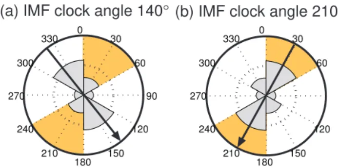
Fig. 1. Event selection strategy. The gray areas show the inte-grated amount of energy transfer on the magnetopause surface in six azimuthal sectors during IMF clock angle of(a)θ=140◦and
(b)θ=210◦looking tailwards, and the IMF direction is illustrated with a black arrow. The yellow areas in the diagram illustrate the desired areas of Cluster crossings; in panel(a)Cluster would not observe significant energy transfer while in panel(b) the energy transfer would be increased and the amount and sign would depend on the upstream parameters as well as the exact location of crossing. The energy transfer results are from a previous unpublished run and are here only to facilitate an a priori hypothesis for the investigation.
site. After a field line has been reconnected, it evolves across the magnetopause and is added to the tail lobes of open mag-netic flux in the nightside, where it eventually reconnects and closed flux is created. Therefore, current theory suggests that on the dayside equatorward of the cusp, energy is transferred to the plasma by magnetic reconnection, which represents a load in the system. On the other hand, tailward of the cusp energy is extracted from the motion of the magnetosheath plasma and converted to magnetic energy, making hence the tail magnetopause a generator. While the qualitative pic-ture of the cause and effect of the energy transfer is clear, the quantitative formulation has proven markedly difficult. Mostly, the global energy transfer estimates rely on correla-tions of the solar wind parameters to magnetospheric activity indices (Akasofu, 1981; Newell et al., 2007). However, such proxies of the energy transfer lack spatial information of the process and the magnitude of the transferred energy is ap-proximated from the magnetospheric response.
Using a global MHD simulation GUMICS-4, Palmroth et al. (2003, 2006) found a general temporal correspondence to the energy transfer proxies, but also found a distinct spa-tial variation in the energy transfer, where the energy trans-fers in a plane of the IMF orientation. That is, if the IMF clock angleθ=tan−1(IMF y/IMF z) is 180◦and the IMF is
purely southward, the energy transfers in the north-south di-rection on the magnetopause, while deviations from the due south orientation shifts the energy transfer spatial distribu-tion. This was explained by Poynting flux focussing (Pa-padopoulos et al., 1999; Palmroth et al., 2003), where the electromagnetic energy focusses towards the magnetopause in the plane of the IMF and deviates away from the
mag-netopause in a plane perpendicular to the IMF orientation. Mathematically, the Poynting flux focussing is complemen-tary to the load-generator mechanism (Palmroth et al., 2010) and it is enabled because the Poynting vector at the magne-topause surface is nonzero in areas where the open field lines advect tailwards. While the spatial variation of the energy transfer is a trivial consequence of the Poynting theorem, it has never been observationally verified on the magnetopause surface.
An important step towards quantitative energy transfer es-timates were taken by Rosenqvist et al. (2006, 2008b), who presented a method to compute energy conversion within the magnetopause current layer using Cluster observations. Later, they compared the Cluster results with ones obtained from a global MHD simulation (Rosenqvist et al., 2008a). In this paper we carry on with their methodology to investigate the spatial energy transfer distribution on the magnetopause but compare the results to another global MHD simulation. Our strategy is illustrated in Fig. 1: Based on earlier global MHD simulation results, the energy transfer occurs in the plane of the IMF such that for example during IMF clock angle isθ=140◦ (210◦), the energy transfers in the north-ern dawn and the southnorth-ern dusk (northnorth-ern dusk and southnorth-ern dawn) portions of the magnetopause, predominantly sunward ofx= −10RE(Palmroth et al., 2003, 2006). We search for event pairs in which the upstream parameters are otherwise the same and steady, but for which the IMF y-component is equal but of different sign. The steady upstream conditions are desired as the pressure variations affect the local energy transfer values, while the different sign in IMF y shifts the energy transfer pattern on the magnetopause as illustrated in Fig. 1. From the event pairs, we take only events where the Cluster constellation crosses the magnetopause within the same area, and for which the separation is preferably such that it allows the determination of the current density using the accurate curlometer technique (Dunlop et al., 2002). We expect that for an event similar to that in Fig. 1a, Cluster would not observe much energy conversion, while in an event depicted in Fig. 1b significant energy conversion would be observed.
θCluster=36◦for 26 January 2001). The paper is organized as follows: first, we briefly review the methodology for in-ferring the energy transfer from the global MHD simulation as well as from Cluster observations. Second, we investigate the two Cluster magnetopause crossings in detail and present the performed simulations. Finally, we compare the simu-lation results on the energy transfer to those obtained from Cluster observations, and end the paper with discussion and conclusions. Overall, GSE coordinates are used in this paper.
2 Methodology
2.1 GUMICS-4
GUMICS-4 (Janhunen, 1996) is a state-of-the-art global MHD simulation that solves the fully conservative MHD equations within the the simulation box extending from +32RE to −224RE in x-direction and±64RE in the yz-directions. The magnetospheric domain is coupled with an electrostatic ionosphere: The magnetosphere determines the field-aligned currents and electron precipitation, which are given as boundary conditions to the ionospheric simulation domain. The field-aligned currents and the conductivity pat-tern resulting from precipitation and solar irradiation are used to determine the electric potential, which is given back to the magnetosphere, where it is used as an ionospheric bound-ary condition. Solar wind density, velocity, temperature and magnetic field are introduced as an input to the code at the sunward wall of the simulation box, while a variety of quan-tities are given as an output of the computation in space and time. GUMICS-4 uses a cell-by-cell adaptive grid, where the cells are divided into two at places with large spatial gradi-ents.
Palmroth et al. (2003) introduced a method with which the global energy transfer can be investigated using the GUMICS-4 simulation. The method first identifies the mag-netopause boundary, and then computes the simulation to-tal energy flux perpendicular to the surface and defines this as the transferred energy. The GUMICS-4 magnetopause surface coincides with the statistical magnetopause location (Shue et al., 1997, 1998), and the method has also been found to work in other simulation runs (Shukhtina et al., 2009) us-ing the OpenGGCM code (e.g., Raeder, 2003).
The total energy perpendicular to the magnetopause boundary is defined as the portion of energy through the mag-netopause as
Pmp= Z
A
K·ndA, (1)
whereK is the total energy flux (kinetic + thermal + elec-tromagnetic) in the GUMICS-4 simulation determined at the surface of the magnetopause,nis the unit normal vector of the surface pointing outwards, anddAis the area of the sur-face element. In this paper, the general term “energy
trans-fer” refers to Eq. (1). The computation requires that the sur-face is identified for each time instant, and the integration proceeds from the nose to −30RE in the tail. The mag-netopause can be divided in smaller integration domains to study the spatial distribution of energy transfer, and one con-venient way to do this is given by
PAZ(1φ)=
Z
1φ
Z −30
x=nose
K·ndA(φ,x), (2)
where the integration is carried out from nose to the−30RE in sectors 1φ that are defined similarly as the IMF clock angle (zero in the north, 180◦in the south). For example, the
energy transfer spatial distribution on the magnetopause in Fig. 1 is illustrated using Eq. (2) in 6 azimuthal bins (1φ= 60◦), and shown as polar histograms for the prevailing clock angle.
Laitinen et al. (2006, 2007) introduced a method to evalu-ate the magnetopause dynamo and reconnection powers at the magnetopause from the GUMICS-4 simulation. They computed the “energy conversion surface density”, given by
Pec= − Z l2
−l1
∇ ·Sdl, (3)
where the subscript “ec” denotes energy conversion,Sis the Poynting vector, and the integration is carried out along the magnetopause normal through the magnetopause layer from −l1tol2. Essentially, Eq. (3) computes how much magnetic energy is destroyed in the dayside reconnection region and how much magnetic energy is generated within the lobe dy-namo converting the solar wind kinetic energy into magnetic energy. In this paper, a general term “energy conversion” in simulation refers to Eq. (3).
2.2 Cluster instruments and methods
In a time-independent case, a straightforward calculation shows that
−∇ ·S=E·J=J×B·v (4) whereE is the electric field,J is current density,Bis mag-netic field, and v is plasma velocity. Using Eq. (4), it is possible to compute the energy conversion from spacecraft observations during a magnetopause crossing (Rosenqvist et al., 2006). Now, the integration lengthdlis converted into dl= |vmp|dt, where the vmp is the magnetopause velocity with respect to the spacecraft and thedtis the duration of the current layer crossing. Hence, the energy conversion during a magnetopause crossing is evaluated as
Q=
Z
(J×B)·v|vmp|dt. (5)
use the absolute value of the velocity. This is because the sign of the integrand must choose the sign of the energy conver-sion and the integration measuredl= |vmp|dt only decides the size of the subareas to be summed in the final integral.
In this paper, Eq. (5) is evaluated using Cluster space-craft observations. The magnetic field and plasma veloc-ity are directly obtained from the Flux-Gate Magnetometer (FGM, Balogh et al., 2001) and Cluster Ion Spectrometer (CIS, R`eme et al., 2001). The current density is computed using the curlometer technique (Dunlop et al., 2002), where the current density is obtained from Amp`ere’s law and the curl of the magnetic field is computed using the observed spatial gradients within the spacecraft constellation (tetrahe-dron). The curlometer technique gives the most reliable esti-mates of the current amplitude and direction in cases where the spacecraft separation is smaller than the scale length at which the current density varies, and where the tetrahedron is not elongated but equally separated (Dunlop et al., 2002).
For the velocity of magnetopause, both multi-spacecraft methods based on timing analysis as well as single space-craft methods are available. The relative timing of the four spacecraft observations can be used in determining the ve-locity and orientation of any discontinuity. Here we use constant velocity approach (CVA) assuming that the mag-netopause moves at a constant speed during the constellation fly-by. The relative timings of the magnetopause crossings are found by correlating similar structures, and the orien-tation and velocity of the discontinuity are then computed from the timings (Dunlop and Woodward, 1998). For the single-spacecraft methods, Sonnerup et al. (2006) introduced a generic residue analysis (GRA) method, where classical conservation laws are used to determine the orientation and motion of a plasma discontinuity. The method includes con-servation laws for mass, momentum, total energy, entropy, magnetic flux, and electric charge, and gives results for each conservation law. The optimal value for the orientation and motion of the discontinuity is obtained by weighting.
3 Event descriptions
3.1 Upstream conditions
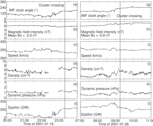
Figure 2 presents the upstream conditions for the two se-lected events. Advanced Composition Explorer (ACE) solar wind Level 2 data are presented for the periods of 16 January 2001 (left panels) and 26 January 2001 (right panels), and a delay of 71 min and 69 min from the ACE position to 15RE is added, respectively. The IMF observations are recorded by the magnetic field instrument (MAG) (Smith et al., 1998), while the solar wind density and velocity are determined by the Solar Wind Electron Proton Alpha Monitor (SWEPAM) instrument (McComas et al., 1998). The vertical lines denote the Cluster magnetopause crossings examined in this paper. Both crossings occur during relatively steady solar wind, and
hence the exact determination of the delays added to the ACE recordings is not crucially important. The IMF intensity and solar wind density and velocity in the two events are almost identical. The significant difference during the events is that the IMF y-component is almost as much positive during the Cluster magnetopause crossing on 16 January as it is nega-tive during the crossing at 26 January, making the clock an-gleθduring the events almost symmetric with respect to due south (∼166◦ and 224◦). Furthermore, during 26 January, the IMF is steadily southward for several hours prior to the time of interest, while on 16 January the IMF is northward for several hours prior to the Cluster magnetopause crossing. Theǫparameter computed from the upstream parameters in the events is the same,∼200 GW at the times of the magne-topause crossings. As will be shown later, the time period during which the IMF is southward prior to the events is suf-ficiently long so that the energy transfer distribution has had time to develop at the magnetopause.
3.2 Magnetopause crossing on 16 January 2001
400
200
0 2 1 0 3 4 2 6 10 8 400
350
300 4 2 6
0 8 240
120
0 360
07:00 08:00 09:00 10:00
Time of 2001-01-26 Epsilon (GW)
Dynamic pressure (nPa) Density (cm-3)
Speed (km/s)
Magnetic field intensity (nT) Mean Bx = -0.8 nT
IMF clock angle (°) Cluster crossing
20:00 21:00 22:00 23:00 Time of 2001-01-16
Cluster crossing
Epsilon (GW)
Dynamic pressure (nPa) Density (cm-3)
Speed (km/s)
Magnetic field intensity (nT) Mean Bx = -2.0 nT
IMF clock angle (°)
(a)
(b)
(c)
(d)
(e)
(f)
(g)
(h)
(i)
(j)
(k)
(l)
11:00
Fig. 2. Four hours worth of Advanced Composition Explorer (ACE) solar wind observations on 16 January 2001 (left panels), and on 26 January 2001 (right panels). A delay of 1 h 11 min and 1 h 9 min from ACE position to +15REhas been added, respectively.(a)and(g)IMF
clock angle in the yz-plane,(b)and(h)magnetic field intensity,(c)and(i)solar wind speed,(d)and(j)solar wind density,(e)and(k)dynamic pressure, and(f)and(l)ǫparameter computed using the solar wind parameters. The vertical lines denote the Cluster magnetopause crossings on each day.
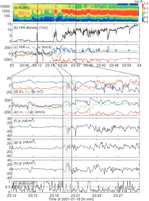
when this ratio is smaller than 0.5 (Dunlop et al., 2002). The period from 23:12 UT until 23:19 UT shows positiveBz component, whileBxis negative, indicating that Cluster was crossing the dayside magnetopause equatorward of the cusp. The At 23:19 UT, an anti-sunward, duskward and northward current is observed, and the magnetic field rotates reaching values of the magnetosheath magnetic field. The curlometer quality factor in Fig. 3g shows that except for a few points, the current estimate is reliable.
Next, we estimate the magnetopause normal and velocity for the 16 January event. The first block of Table 1 shows the results of the single-spacecraft analysis of the magnetopause normal, de Hoffman-Teller velocity, and magnetopause ve-locity in the normal direction. The largest ratio of the in-termediate and normal eigenvalues is given by the MVAB method. The velocity of the magnetopause in the normal direction is around−20 km s−1for the methods using mag-netic field records. Since the spacecraft velocity is negligible compared to the magnetopause velocity, the magnetopause
moves inward over the spacecraft during this outbound cross-ing; i.e., the velocity direction is opposite to the outward pointing normal vector, explaining the negative sign in the magnetopause velocity. We also performed the CVA analy-sis for the magnetopause crossing using the magnetic field Lcomponent in the boundary layer frame (using the MVAB normal from spacecraft 1) from all four spacecraft around the 23:19 UT. The results for the multi-spacecraft analysis are given in the second block of Table 1. The multi-spacecraft analysis is consistent with the MVAB analysis, suggesting that the magnetopause velocity during the event is around −30 km s−1. We use both these values in the rest of the pa-per.
3.3 Magnetopause crossing on 26 January 2001
15 10 5 0
200 0 -200
20
0
-20
200 0 -200
20 0 -20 40
-40
20 0 -20 40
-40
20 0 -20 40
-40 1
0 0.5
23 24
23:12 23:15 23:18 23:21 23:24 23:27
Time of 2001-01-16 [hr:min]
23:06 23:12 23:18 23:24 23:30 23:36 23:42 23:48 23:54
(i) divB/curlB (d) Bx, By, Bz (nT)
(e) vx, vy, vz (km/s)
(f) jx (nA/m2)
(g) jy (nA/m2)
(h) jz (nA/m2) 10000
1000 100
(a) E (eV)
2.9 4.0 5.1 6.2 7.3 log JE
(b) HIA density (1/cc)
(c) HIA vx, vy, vz (km/s)
Fig. 3.Cluster spacecraft 1 observations on 16 January 2001. (a)Omnidirectional proton energy spectrogram,(b)density and(c)velocity GSE components (x-, y- and z-components on red, green and blue, respectively) from CIS/HIA. The black vertical lines indicate a time period for which the panels(d)–(i)are presented:(d)Magnetic field GSE components from FGM,(e)velocity of plasma (CIS),(f)–(h)x-, y- and z-components of current density (curlometer), and(i)the curlometer quality factor. The gray rectangle shows the exact time period of the crossing in question.
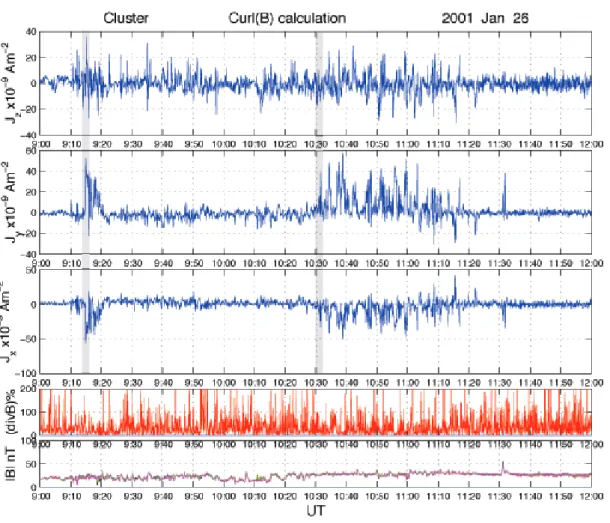
Even though in January 2001 the Cluster tetrahedron is quite elongated, (Dunlop et al., 2002) used the event as an example of a case where the current density can still be accurately de-termined using the curlometer technique. Figure 4 presents the curlometer current density components, the curlometer quality factor and the magnitude of the magnetic field from 09:00 UT until 12:00 UT. During the plotted period the di-rection of the current is northward, duskward, and tailward at most of the magnetopause crossings, indicating that the
Table 1. Magnetopause normal and velocity analysis for 16 January 2001; time interval 23:18:48 UT to 23:20:28 UT. Ratio is the ratio of intermediate and normal eigenvalue given by the analysis,vHTis the de Hoffman Teller velocity, andvHT·ngives the magnetopause velocity in the normal direction.
Method Ratio vHT Normal vHT·n(km s−1)
Minimum variance (MVAB) 11.4 (−186.5,−1.6, 116.3) (0.57 0.31 0.76) −17.9
Minimum Faraday residue (MFR) 10.2 (−145.1, 84.4, 40.7) (0.55 0.33 0.77) −20.5
Minimum mass flux residue (MMR) 4.8 (−228.6, 103.0, 84.3) (0.93 0.09 0.36) −171.8
Minimum entropy residue (MER) 4.6 (−229.5, 103.4, 84.3) (0.93 0.09 0.37) −171.6
Combined (MVAB, MFR, MMR, MER) 3.4 (−193.4, 59.0, 86.3) (0.74 0.27 0.62) −72.6
Constant velocity analysis (CVA) (0.66 0.32 0.67) −24.1
Fig. 4.The current density inferred using the curlometer technique, from 09:00 UT until 12:00 UT at 26 January 2001. Highlighted in grey are two magnetopause crossing, at 09:15 UT and 10:30 UT.
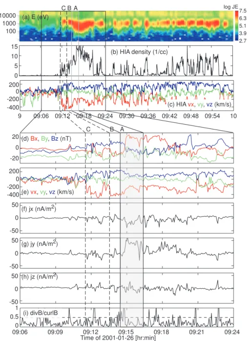
Figure 5a–c present one hour of data on 26 January 2001, from Cluster spacecraft 1 at approximately [3.5 6.7 9.1]RE, in the same format as in Fig. 3. According to Bosqued et al. (2001), the core magnetosheath population is observed at 09:17 UT (after the second gray vertical line in Fig. 5a– c). The transition from the magnetosphere into the core magnetosheath population occurs through a boundary layer,
These observations indicate that the jets are associated with the structure of the boundary layer during the event.
Figure 5d–i shows 18 min worth of data around the mag-netopause crossing in the same format as in Fig. 3d–i. The period from 09:06 UT until 09:11 UT is associated with al-most zeroBx, and negativeBz, indicating a dayside crossing equatorward of the cusp. At about 09:15 UT, the magnetic field rotates, the velocity components show a distinct change, and the current density shows an anti-sunward, duskward and northward increase consistent with the Chapman-Ferraro current direction circulating the cusps in the post-noon sec-tor. Notice that during most of the skimmings of the bound-ary layer, such as at 09:23 UT, the current direction is anti-sunward, dawnward, and northward. This current direction is parallel to the B×v electric field, and hence we argue that the current signature observed during these periods is not the Chapman-Ferraro system, but is associated with the high-velocity jets.
We performed a similar single spacecraft and multi space-craft boundary orientation and velocity analysis as for the 16 January case. The results are presented in Table 2. As the crossing does not occur from the magnetosphere proper into the sheath proper, the quality of the results are not as good as in the 16 January case. The MVAB method yields again the largest eigenvalue ratio. The CVA timing analysis is difficult as all four spacecraft do not cross the entire magnetopause layer. However, we performed the timing analysis using the first clear magnetosphere-to-boundary layer magnetic struc-ture, and obtained a value of −58 km s−1 for the magne-topause velocity. The value is similar to the one found in Bosqued et al. (2001), who obtained−40 km s−1using both single- and multi-spacecraft methods later during the same day, at 10:30 UT. As the duration of the 09:15 UT crossing is also similar to the 10:30 UT crossing, we use in the rest of the analysis the value−40 km s−1, agreeing sufficiently well with the CVA and MVAB.
4 GUMICS runs
GUMICS-4 was executed with the solar wind input from the periods given in Fig. 2. The smallest grid spacing in the simulation runs is 0.25RE, ensuring a sharp boundary at the magnetopause. Due to the code setup where the solar wind magnetic field needs to be divergenceless, solar windBxwas set to zero. The dipole tilt angle in both runs is set to zero, otherwise the code setup is typical that has been used in sev-eral event simulations (e.g., Palmroth et al., 2003). There are indications that the IMFBxand the tilt angle affect the re-connection line location (e.g., Trenchi et al., 2008) and hence the approximations for the tilt angle and the IMFBxmight be invalid in investigations of the load and generator areas. However, as the negative tilt in January and the negative IMFBxshift the reconnection line into opposite directions, and the negative tilt has only a slight effect in the
North-ern Hemisphere where the Cluster crossings occur (Palmroth et al., 2011), the assumptions concerning the tilt and IMF Bx are valid. Figure 6 illustrates the Cluster orbits on 16 January (left panels) and 26 January (right panels) overlaid with GUMICS-4 reproduction of the plasma density for both events.
5 Results: energy transfer and conversion on magnetopause
Figure 7 shows the total energy computations and azimuthal energy distributions for the 16 January event. The temporal variation of the total energy transfer through the GUMICS-4 magnetopause resembles that of the ǫ parameter, while the magnitudes are different. This is due to the fact thatǫ is scaled to the magnetospheric energy consumption, while the GUMICS-4 energy transfer (Eq. 1) includes all energy transferred through the surface untilx= −30RE, which is not necessarily deposited within the ionosphere or the inner magnetosphere. Therefore, Fig. 7b also shows theǫ parame-ter scaled with the simulation magnetopause mean area (red) during the run instead of the traditional 4π l20scaling param-eter, wherel0=7RE. The vertical lines in Fig. 7b denote the time instants at which we present azimuthal energy transfer distributions shown in Fig. 7c computed using Eq. (2). Theφ axis at the outer circle shows the magnetopause in yz-plane looking tailward, and the energy transfer through each sector 1φis given by a bar, whose size is proportional to the energy input in that sector, normalized to the outer circle (100 GW). The black line and dot in each energy distribution shows the IMF orientation and clock angle.
15 10 5 0 200
0 -200
20
0
-20
200 0 -200
0 50
-50
1
0
0.5 (i) divB/curlB (d) Bx, By, Bz (nT)
(e) vx, vy, vz (km/s)
(f) jx (nA/m2)
(g) jy (nA/m2)
(h) jz (nA/m2)
(b) HIA density (1/cc)
(c) HIA vx, vy, vz (km/s) -400
-400
9 09:06 09:12 09:18 09:24 09:30 09:36 09:42 09:48 09:54 10
0 50
-50
0 50
-50
09:06 09:09 09:12 09:15 09:18 09:21 09:24
Time of 2001-01-26 [hr:min]
2.7 3.9 5.1 6.3 7.5 log JE
10000 1000 100
(a) E (eV) B
C A
B
C A
Fig. 5.Cluster spacecraft 1 observations on 26 January 2001, from spacecraft 1.(a)Omnidirectional proton energy spectrogram,(b)density and(c)velocity GSE components (x-, y- and z-components on red, green and blue, respectively) from CIS/HIA. The black vertical lines indicate a time period for which the panels(d)–(i)are presented: (d)magnetic field GSE components from FGM,(e)velocity of plasma (CIS),(f)–(h)x-, y- and z-components of current density (curlometer), and i) the curlometer quality factor. The gray rectangle, vertical dashed lines and letters A, B and C refer to Table 3.
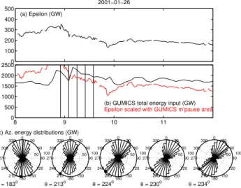
Figure 8 shows the ǫparameter, total energy transfer in GUMICS-4 as well as the azimuthal energy transfer distri-butions for 26 January, in the same format as in Fig. 7. The vertical lines are now showing the time instants separated by 10 min, and centered by the Cluster magnetopause cross-ing that took place about 09:15 UT. Again, the energy trans-fers in the plane of the IMF, and the distributions in Fig. 8c stay qualitatively similar at an after 09:15 UT, although the
Table 2.Magnetopause normal and velocity analysis for 26 January 2001; time interval 09:14:30 UT to 09:15:20 UT. The format is the same as in Table 1.
Method Ratio vHT Normal vHT·n(km s−1)
Minimum variance (MVAB) 3.3 (−321.6 68.9 145.7) (0.45−0.20 0.87) −33.3
Minimum Faraday residue (MFR) 2.4 (−73.9 161.4 41.3) (0.42−0.01 0.91) 5.2
Minimum mass flux residue (MMR) 1.0 (−36.1 82.7 25.4) (0.54−0.83 0.16) −83.9
Minimum entropy residue (MER) 1.1 (−21.0 87.8 16.1) (0.54−0.82 0.15) −81.4
Combined (MVAB, MFR, MMR, MER) 2.5 (−253.4 90.9 116.9) (0.44−0.12 0.89) −19.0
Constant velocity analysis (CVA) (0.60 0.33 0.73) −58.2
Fig. 6.Cluster spacecraft positions (magenta circles) on 16 January (panelsaandb), and 26 January (panelscandd) during the period presented in Fig. 2. The colorcoding is the GUMICS-4 reproduction of logarithm of plasma density during the two events. Panels(a)and
(c)are depicted in xy-plane atz=0, whereas panels(b)and(d)are those for yz-plane atx=0.
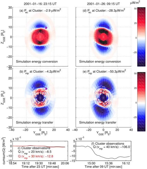
Figure 9 shows the results of the detailed comparison be-tween the GUMICS-4 simulation against the Cluster esti-mate of the energy conversion, calculated using the data from times highlighted with gray in Figs. 3 and 5. The left (right) panels are again for 16 January (26 January) events. The top row shows the GUMICS-4 energy conversion computed us-ing Eq. (3), while the second row gives the energy transfer using Eq. (1). The magnetopause is viewed from the front looking tailwards. The magenta dots give the Cluster posi-tion in each event at the given time. The GUMICS-4 results on the energy conversion and transfer at the Cluster posi-tion are given in the respective legends of Fig. 9a–b and 9d– e. The GUMICS-4 results for 16 January are evaluated at 23:15 UT, and 09:15 UT on 26 January. The energy transfer distributions depicted in Fig. 9b and 9e are almost as much tilted with respect of due south and show almost similar mag-nitudes of energy transfer as the other solar wind conditions
0 100 200 300 400 500
(a) Epsilon (GW)
2001−01−16
21 22 23 24
0 500 1000 1500 2000
(b) GUMICS total energy input (GW)
Epsilon scaled with GUMICS m’pause area (GW)
50 100 30
210 60
240
90 270
120 300
150 330
180 0
θ = 116o
(c) Az. energy distributions (GW)
50 100 30
210 60
240
90 270
120 300
150 330
180 0
θ = 136o
50 100 30
210 60
240
90 270
120 300
150 330
180 0
θ = 151o
50 100 30
210 60
240
90 270
120 300
150 330
180 0
θ = 161o
50 100 30
210 60
240
90 270
120 300
150 330
180 0
θ = 166o
Fig. 7. (a)Theǫparameter for 16 January event, delayed to +15RE
using a delay 1 h 11 min. (b) Total energy transfer through the magnetopause in the GUMICS-4 simulation against time in the 16 January event (black) andǫparameter scaled with the simulation magnetopause area (red). Vertical lines denote the times at which the instantaneous energy transfer distributions in(c)are given. The size of the bar in panels(c)gives the portion of energy transfer in the yz-plane integrated from the nose to−30RE. The bar size is
normalized to the outer circe (100 GW), and the IMF orientation is given by the black line, with the filled dot referring to the clock angle given in the bottom left legend of each distribution.
are similar. The bottom row gives the Cluster estimate of the energy conversion Qusing Eq. (5) in the two events. The integral of the energy conversion through the magnetopause is computed as a cumulative sum, and hence the final value of the plotted curve given in the legend of Fig. 9c, f is to be compared with the simulation results. The Cluster estimate for 16 January is computed using two values for the mag-netopause velocity: 20 km s−1(black) and 30 km s−1 (red), while the value for 26 January uses 40 km s−1 found here and in Bosqued et al. (2001).
Table 3.Cluster estimations of the energy conversion using different time intervals and including all current density values in the calculation (Q1) and omitting those current density values where the curlometer quality factor is larger than 0.5 (Q2). The difference (%) tells how
muchQ1differs fromQ2.
Time Q1(µW m−2) Q2(µW m−2) vmp(km s−1) Difference
16 January 2001
23:18:36–23:20:27 UT −8.6 −5.3 20 38 %
23:18:36–23:20:27 UT −12.8 −8.0 30 38 %
26 January 2001
A: 09:14:27–09:16:23 −106.4 −95.9 40 10 %
B: 09:13:30–09:16:23 −102.1 −89.1 40 13 %
C: 09:11:31–09:16:23 −130.0 −114.3 40 12 %
0 100 200 300 400 500
(a) Epsilon (GW)
2001−01−26
8 9 10 11
0 500 1000 1500 2000 2500
(b) GUMICS total energy input (GW)
Epsilon scaled with GUMICS m’pause area
50 100 30 210 60 240 90 270 120 300 150 330 180 0
θ = 183o
(c) Az. energy distributions (GW)
50 100 30 210 60 240 90 270 120 300 150 330 180 0
θ = 213o
50 100 30 210 60 240 90 270 120 300 150 330 180 0
θ = 224o
50 100 30 210 60 240 90 270 120 300 150 330 180 0
θ = 230o
50 100 30 210 60 240 90 270 120 300 150 330 180 0
θ = 234o
Fig. 8. (a)Theǫparameter for 26 January event, delayed to +15RE
using a delay 1 h 9 min.(b)Total energy transfer through the mag-netopause in the GUMICS-4 simulation against time in the 26 Jan-uary event (black) andǫparameter scaled with the simulation mag-netopause area (red). Vertical lines denote the times at which the instantaneous energy transfer distributions in(c)are given. The for-mat of the figure is the same as Fig. 7.
the north-south direction, and occurs in the northern dawn and southern dusk sectors at the magnetopause. The Cluster crossing of the magnetopause occurs in between the load and generator regions away from the strongest energy conversion and transfer, and indeed in Fig. 9c the Cluster estimate of the energy conversion within the magnetopause current layer is small, only from−8 to −13 µW m−2. The Cluster esti-mate is larger than in GUMICS, but still in quantitative ac-cordance with the simulation results: The simulation shows little energy conversion and transfer, as the conversion esti-mate is about−3 µW m−2 and transfer about −4 µW m−2. The pixels neighboring the Cluster crossing location give similar magnitudes, but can be of different sign. On 26
Jan-uary, however, Cluster crosses the magnetopause in a region where the simulation results indicate large energy conversion and transfer. Based on the simulation, the location of the crossing occurs well within the generator region as now the neighboring pixels show similar magnitudes and sign for en-ergy conversion, indicating also that our initial assumptions of the tilt angle and IMFBxare valid. The simulation esti-mates for the conversion and transfer are−28 µW m−2 and −50 µW m−2, respectively, lower than the Cluster estimate, which is−106 µW m−2. In both events, the Cluster estimate of the energy conversion exceeds that of the GUMICS-4 lo-cal energy conversion by the same factor∼4.
Table 3 gives Cluster estimations of the energy conversion from the two events using different crossing parameters. The 16 January crossing is “clean”, such that there is no ambigu-ity on the timing of the crossing, and as indicated by Fig. 3, the spacecraft traverses from the magnetospheric-like into sheath-like population rapidly without observing a boundary layer. The ambiguity within the crossing comes from the ex-act value of the magnetopause velocity, and the few points of possibly erroneous curlometer current density measure-ments. Hence, we present theQcalculation using the two magnetopause velocity values as well as omitting the data points having a larger curlometer quality factor than 0.5. The valueQ1 is hence computed using all points from the time period, but in computing the valueQ2the points where the curlometer quality factor exceeds the 0.5 limit are set to zero. As the GUMICS-4 result was−2.9 µW m−2, the Cluster es-timate is larger by a factor of 2–3.
−30 −20 −10 0 10 20 30
2001−01−16: 23:15 UT
(a) P
ec at Cluster: −2.9 µW/m
2
Simulation energy conversion
Z GSE
[R
E
]
−40 −20 0 20 40
−30 −20 −10 0 10 20 30
Y
GSE [RE] (b) P
mp at Cluster: −4.2µW/m
2
Simulation energy transfer
Z GSE
[R
E
]
18:54 19:12 19:30 19:48 20:06
−15 −10 −5 0
5x 10
−5
Time after 23 UT [min:sec]
cumsum(Q) [W/m
2 ]
c) Cluster observations Q (v
mp = 20 km/s): −8.5
Q (v
mp = 30 km/s): −12.8
2001−01−26: 09:15 UT
(d) P
ec at Cluster: −28.3µW/m
2
Simulation energy conversion
−25 0 25 50
µW/m2
−40 −20 0 20 40
Y
GSE [RE] (e) P
mp at Cluster: −50.3µW/m
2
Simulation energy transfer
−25 0 25 50
15:00 15:36 16:12
−15 −10 −5 0
5x 10
−5
Time after 09 UT [min:sec] Q (v
mp = 40 km/s): −106.0
(f) Cluster observations
Fig. 9.Left (right) panels: results for 16 January at 23:15 UT (26 January at 09:15 UT).(a)and(d)divergence of the Poynting vector at the magnetopause surface in the GUMICS-4, looking tailwards from the front of the magnetopause.(b)and(e)total energy transfer through the magnetopause surface in the GUMICS-4.(c)and(f)Cumulative sum (representing the time evolution of theQintegral) of energy conversion at Cluster orbit through the magnetopause; red (black) curve usingvmp=20 (30) km s−1for 16 January. The magenta dots in panels(a),(b),
(d)and(e)show the Cluster position on the given time, and the values in the respective legends show the simulation result on Cluster position at the given time. The Cluster estimate of the integral of the energy conversion (the final value of the cumulative sum) in the magnetopause current layer is given in the legends of panels(c)and(f). All values in legends are given in µW m−2
about−100 µW m−2, again larger by a factor of 3 compared to the GUMICS-4 local values. Hence in both events, am-biguity of the measurements explained a factor of 1 discrep-ancy between the measurements and the simulation results, but the same scaling factor of 2–3 was found between the Cluster observations and the simulation results.
6 Discussion
results. We find the same scaling parameter (a factor of 2–3) from both local estimates. We have also briefly reviewed the methodology developed earlier to infer the simulation energy transfer and conversion from GUMICS-4 global MHD simu-lation (Palmroth et al., 2003; Laitinen et al., 2006, 2007). The two methods represent two complementary viewpoints in the magnetopause energetics and they are both consequences of the dayside magnetopause reconnection. The energy trans-fer method tells us how much total energy (kinetic, electro-magnetic and thermal) transfers across the magnetopause, while the energy conversion method yields an estimate of how much of the transferring energy is converted from one form to another, and directly evaluates the power consumed by reconnection. Hence in principle, the magnitude of en-ergy conversion cannot exceed that of the enen-ergy transfer. The spatial variation of the transfer and conversion is not necessarily exactly the same as the integrals are different, although using primarily the same quantities. The energy conversion occurs primarily within or adjacent to the recon-nection region, but energy can transfer (via Poynting flux fo-cussing) anywhere on the surface, where open field lines ex-ist. The energy conversion method should be comparable to the Cluster methodology (Rosenqvist et al., 2006) in a time-independent case, as shown by Eq. (4). Time-independency is a good assumption if the magnetopause structure remains steady during the event. This is the case in both of the events discussed here.
In computing the Cluster estimate of the magnetopause en-ergy conversion, obvious sources of errors include the deter-mination of the current density and the magnetopause veloc-ity. Especially the latter is a constant multiplier in Eq. (5) and order-of-magnitude errors would introduce an order of mag-nitude discrepancy in the final estimation. Here, we have carefully measured the velocity of the magnetopause. We have also used the best available method (curlometer) to in-fer the current density, and we note that the single space-craft methods yield similar values (not shown). Hence, our current density estimate is generally reliable, while instan-taneous observations include uncertainties that lead to dis-crepancies within the final estimate (Table 3). As witnessed during the 26 January 2001 event, the magnetopause can in-clude local effects that are associated with boundary layer dynamics. Hence, we argue that the timing should be done as carefully as possible, so that only the large scale Chapman-Ferraro current contributes toQ. Special care should be paid on the timing of the event if it includes spiky current density features that are not consistent with the large-scale current direction. However, one of the most important finding of this paper is that even with the best possible means to infer energy conversion (multi-spacecraft techniques, carefully selected events and stable upstream conditions) an uncertainty factor exists within the observations. Here, the final estimates in-clude 10 %–40 % differences, which were due to timing, ve-locity of the magnetopause as well as momentary bad values of the curlometer. We envisage that in more dynamic events
having unstable upstream conditions, the discrepancies can be larger.
The 26 January case was also one of many crossings anal-ysed by Rosenqvist et al. (2008b,a). They +67 µW m−2for Qat 10:30 UT and interpreted the event as being a cross-ing of the load region. Uscross-ing the BATS-R-US global MHD simulation, Rosenqvist et al. (2008a) computed bothQand −∇ ·S from the simulation results along the Cluster orbit. The comparison yielded favorable results only after they ar-tificially lowered the spacecraft trajectory in the simulation towards the subsolar magnetopause. We note that in Rosen-qvist et al. (2008a,b) the a priori assumption on the load na-ture of the crossing was made based on the current theoreti-cal understanding that the load exists equatorward of the cusp (Lundin and Evans, 1985). However, most importantly, the current density during the 10:30 UT event shows southward signatures, while typically the magnetopause crossings on 26 January show northward current densities (Fig. 4). Flipping the sign of theJzto positive at 10:30 UT flips the sign ofQ into negative, consistent with our findings of the 09:15 UT crossing. Since the current shows northward signatures dur-ing several of the crossdur-ings, we note that the current density direction at 09:15 UT is consistent with the global Chapman-Ferraro direction, while the 10:30 UT crossing possibly in-cludes local signatures that influence the current direction. The global simulations cannot easily reproduce local signa-tures, while the global pattern is reproduced on average. In-deed, Fig. 9 shows a large positive region equatorward of the generator region, and hence the artificial lowering of the spacecraft orbit in a simulation would yield a good agree-ment.
surface, and hence the cusp is a special case of this general condition. While it would be interesting to find this separator, we leave it for further study with a notion that the separator search should start by finding a location where the accelera-tion fields caused by the magnetosheath flow and theJ×B force are in balance. This also introduces interesting avenues for further studies of the magnetopause energy transfer as it suggests that the load and generator regions (their sizes and possibly also their intensities) can be dependent on the mag-netosheath velocity field, which in turn is related not only to the velocity of the solar wind but also to the shock structure. In a global simulation using a quantitative methodology the a priori assumptions are more easily formed as the out-come of the calculation is plainly visible as in Fig. 1, em-phasizing the power of the approach combining the simu-lations with observations. When looking at the simulation data giving a full three-dimensional global picture of the two events, the Cluster estimates fall naturally in place and are almost in quantitative agreement with the simulation results. We believe that here the Cluster estimate and the simula-tion results validate each other: the simulasimula-tions show that the large differences in the Cluster estimates is natural and due to the spatial variation of energy transfer and conversion. On the other hand, the carefully measured Cluster estimate pins down the magnitudes of the simulation results. Assum-ing that the comparison between in situ observations and the simulation is as good also in other parts of the magnetopause, we are able to pin down the total energy transfer during the two time instants. We estimate that the total energy transfer-ring through the magnetopause dutransfer-ring the two events is about 1500–2000 GW, three times the value ofǫ. Theǫrepresents Poynting flux through a circular area of radiusl0, where the radius is used to scale the energy input to equal the magneto-spheric output. To make the simulation results more directly comparable withǫ, we have scaled theǫagain with the mag-netopause mean area during the events, as measured from the simulation. Our results show that the local values in the sim-ulation are underestimated by a factor of probably 2–3, while the scaledǫis in quantitative agreement with the simulation energy input. This indicates thatǫis underestimated based on the evidence of this paper. In accordance, Koskinen and Tanskanen (2001) also suggested in a broad review of theǫ parameter thatǫshould be scaled up by a factor of 1.5–2.
7 Summary and conclusions
We conclude that the GUMICS-4 simulation results are in good agreement with the Cluster observations in these two cases. The magnitude of energy conversion in the simula-tion, obtained by means that are directly comparable to the methodology using the Cluster observations, is around 30 % of the Cluster estimate during both events, without any as-sumptions made on the magnetopause velocity or the rela-tive location of the Cluster magnetopause crossing within the
code. The simulation energy transfer values are around 50 % of the Cluster estimate. However, as the observations also in-clude uncertainties, we conin-clude that using the present grid resolution and within the global framework the comparison is as perfect as it can be.
Our main findings in this paper are the following: 1. Cluster observations verify the simulation results on the
IMFBydependence of the energy transfer on the mag-netopause.
2. To estimate global energy transfer, one should only take current layers being part of the Chapman-Ferraro sys-tem.
3. The separator for load and generator should appear where the Alfv´en velocity equals the magnetosheath ve-locity, and the field line is being dragged by the magne-tosheath flow instead of being accelerated by reconnec-tion.
4. The amount of energy conversion and transfer in GUMICS-4 agrees well with Cluster observations dur-ing the presented events, even though shows probably a factor of 2–3 lower values, however, also the Cluster estimate ofQincludes ambiguities.
5. The combined results from the simulation and Cluster observations suggest that theǫparameter is underesti-mated by a factor of 2–3.
Acknowledgements. The Cluster data have been retrieved from the Cluster Active Archive (CAA), and we thank Harri Laakso and team for maintaining the system. ACE spacecraft recordings are re-trieved from the ACE homepage (http://www.srl.caltech.edu/ACE/). We thank the ACE MAG and SWEPAM PI’s C. W. Smith and D. J. McComas for distributing the Level 2 data freely in the in-ternet. We thank the CDAWeb facility for distributing the data. The research leading to these results has received funding from the Eu-ropean Research Council under the EuEu-ropean Community’s Sev-enth Framework Programme (FP7/2007-2013)/ERC Starting Grant agreement number 200141-QuESpace. The work of MP is sup-ported by the Academy of Finland. MWD is partly supsup-ported by Chinese Academy of Sciences (CAS) visiting Professorship for se-nior international scientists grant no. 2009S1-54 and the Specialized Research Fund for State Key Laboratories of the CAS.
Guest Editor M. Taylor thanks M. Liemohn and A. R. Retin`o for their help in evaluating this paper.
References
Akasofu, S.-I.: Energy coupling between the solar wind and the magnetosphere, Space Sci. Rev., 28, 121–190, 1981.
Axford, W. I. and Hines, C. O.: A unifying theory of high-latitude geophysical phenomena and geomagnetic storms, Can. J. Phys. 39, 1433–1464, 1961.
The Cluster Magnetic Field Investigation: overview of in-flight performance and initial results, Ann. Geophys., 19, 1207–1217, doi:10.5194/angeo-19-1207-2001, 2001.
Bosqued, J. M., Phan, T. D., Dandouras, I., Escoubet, C. P., R`eme, H., Balogh, A., Dunlop, M. W., Alcayd´e, D., Amata, E., Bavassano-Cattaneo, M.-B., Bruno, R., Carlson, C., DiLellis, A. M., Eliasson, L., Formisano, V., Kistler, L. M., Klecker, B., Ko-rth, A., Kucharek, H., Lundin, R., McCarthy, M., McFadden, J. P., M¨obius, E., Parks, G. K., and Sauvaud, J.-A.: Cluster observa-tions of the high-latitude magnetopause and cusp: initial results from the CIS ion instruments, Ann. Geophys., 19, 1545–1566, doi:10.5194/angeo-19-1545-2001, 2001.
Boyle, C. B., Reiff, P. H., and Hairston, M. R.: Empirical
polar cap potentials, J. Geophys. Res., 102(A1), 111–125, doi:10.1029/96JA01742, 1997.
Cooling, B. M. A., Owen, C. J., and Schwartz, S. J.: Role of the magnetosheath flow in determining the motion of open flux tubes, J. Geophys. Res., 106, 18764–18775, 2001.
Dungey, J. W.: Interplanetary field and the auroral zones, Phys. Res. Lett., 6, 47–48, 1961.
Dunlop, M. W. and Woodward, T. I.: Multi-spacecraft discontinuity analysis: orientation and motion, in: Analysis methods for multi-spacecraft data, chapter 11, 271–306, edited by: Paschmann, G. and Daly, P. W., ISSI scientific report SR-001, ESA Publications Division, The Netherlands, 1998.
Dunlop, M. W., Balogh, A., Glassmeier, K.-H., and Robert, P.: Four-point Cluster application of magnetic field analysis tools: The Curlometer, J. Geophys. Res., 107(A11), 1384, doi:10.1029/2001JA005088, 2002.
Janhunen, P.: GUMICS-3: A global ionosphere-magnetosphere coupling simulation with high ionospheric resolution, in: Pro-ceedings of Environmental Modelling for Space-Based Applica-tions, 18–20 September 1996, Eur. Space Agency Spec. Publ., ESA SP-392, 1996.
Koskinen, H. E. J. and Tanskanen, E. I.: Magnetospheric energy budget and the epsilon parameter, J. Geophys. Res., 107(A11), 1415, doi:10.1029/2002JA009283, 2002.
Laitinen, T. V., Janhunen, P., Pulkkinen, T. I., Palmroth, M., and Koskinen, H. E. J.: On the characterization of magnetic recon-nection in global MHD simulations, Ann. Geophys., 24, 3059– 3069, doi:10.5194/angeo-24-3059-2006, 2006.
Laitinen, T. V., Palmroth, M., Pulkkinen, T. I., Janhunen, P., and Koskinen, H. E. J.: Continuous reconnection line and pressure-dependent energy conversion on the magnetopause in a global MHD model, J. Geophys. Res., 112, A11201, doi:10.1029/2007JA012352, 2007.
Lundin, R. and Evans, D. S.: Boundary layer plasmas as a source for high-latitude, early afternoon, auroral arcs, Planet. Space Sci., 33, 1389–1406, 1985.
McComas, D. J., Bame, S. J., Barker, P., Feldman, W. C., Phillips, J. L., Riley, P., and Griffee, J. W.: Solar Wind Electron Proton Alpha Monitor (SWEPAM) for the Advanced Composition Ex-plorer, Space Sci. Rev., 86, 563–612, 1998.
Newell, P. T., Meng, C.-I., and Sibeck, D. G.: Some low-altitude cusp dependencies on the interplanetary magnetic field, J. Geo-phys. Res., 94, 8921–8927, 1987.
Newell, P. T., Sotirelis, T., Liou, K., Meng, C.-I., and Rich, F. J.: A nearly universal solar wind-magnetosphere coupling function in-ferred from 10 magnetospheric state variables, J. Geophys. Res.,
112, A01206, doi:10.1029/2006JA012015, 2007.
Palmroth, M., Pulkkinen, T. I., Janhunen, P., and Wu, C.-C.: Storm-time energy transfer in global MHD simulation, J. Geophys. Res., 108(A1), 1048, doi:10.1029/2002JA009446, 2003. Palmroth, M., Laitinen, T. V., and Pulkkinen, T. I.: Magnetopause
energy and mass transfer: results from a global MHD simu-lation, Ann. Geophys., 24, 3467–3480, doi:10.5194/angeo-24-3467-2006, 2006.
Palmroth, M., Koskinen, H. E. J., Pulkkinen, T. I., Toivanen, P. K., Janhunen, P., Milan, S. E., and Lester, M., Magnetospheric feedback in solar wind energy transfer, J. Geophys. Res., 115, A00I10, doi:10.1029/2010JA015746, 2010.
Palmroth, M., Fear, R., and Laitinen, T. V.: Magnetopause energy transfer dependence on dipole tilt and solar wind parameters: A view from a global MHD simulation, in preparation, 2011. Papadopoulos, K., Goodrich, C., Wiltberger, M., Lopez, R., and
Lyon, J. G.: The physics of substorms as revealed by the ISTP, Phys. Chem. Earth, 24, 189–202, 1999.
Raeder, J.: Global Magnetohydrodynamics – A Tutorial, in: Space Plasma Simulation, edited by: Buechner, J., Dum, C. T., and Scholer, M., Lecture Notes in Physics, vol. 615, Springer Verlag, Heidelberg, 2003.
R`eme, H., Aoustin, C., Bosqued, J. M., Dandouras, I., Lavraud, B., Sauvaud, J. A., Barthe, A., Bouyssou, J., Camus, Th., Coeur-Joly, O., Cros, A., Cuvilo, J., Ducay, F., Garbarowitz, Y., Medale, J. L., Penou, E., Perrier, H., Romefort, D., Rouzaud, J., Vallat, C., Alcayd´e, D., Jacquey, C., Mazelle, C., d’Uston, C., M¨obius, E., Kistler, L. M., Crocker, K., Granoff, M., Mouikis, C., Popecki, M., Vosbury, M., Klecker, B., Hovestadt, D., Kucharek, H., Kuenneth, E., Paschmann, G., Scholer, M., Sckopke, N., Seiden-schwang, E., Carlson, C. W., Curtis, D. W., Ingraham, C., Lin, R. P., McFadden, J. P., Parks, G. K., Phan, T., Formisano, V., Amata, E., Bavassano-Cattaneo, M. B., Baldetti, P., Bruno, R., Chion-chio, G., Di Lellis, A., Marcucci, M. F., Pallocchia, G., Korth, A., Daly, P. W., Graeve, B., Rosenbauer, H., Vasyliunas, V., Mc-Carthy, M., Wilber, M., Eliasson, L., Lundin, R., Olsen, S., Shel-ley, E. G., Fuselier, S., Ghielmetti, A. G., Lennartsson, W., Es-coubet, C. P., Balsiger, H., Friedel, R., Cao, J.-B., Kovrazhkin, R. A., Papamastorakis, I., Pellat, R., Scudder, J., and Sonnerup, B.: First multispacecraft ion measurements in and near the Earth’s magnetosphere with the identical Cluster ion spectrometry (CIS) experiment, Ann. Geophys., 19, 1303–1354, doi:10.5194/angeo-19-1303-2001, 2001.
Rosenqvist, L., Buchert, S., Opgenoorth, H., Vaivads, A., and Lu, G.: Magnetospheric energy budget during huge geomagnetic ac-tivity using Cluster and ground-based data, J. Geophys. Res., 111, A10211, doi:10.1029/2006JA011608, 2006.
Rosenqvist, L., Opgenoorth, H. J., Rastaetter, L., Vaivads, A., and Dandouras, I.: Comparison of local energy conversion estimates from Cluster with global MHD simulations, Geophys. Res., Lett., 35, L21104, doi:10.1029/2008GL035854, 2008a.
Rosenqvist, L., Vaivads, A., Retin`o, A., Phan, T., Opgenoorth, H. J., Dandouras, I., and Buchert, S.: Modulated reconnec-tion rate and energy conversion at the magnetopause under steady IMF conditions, Geophys. Res., Lett., 35, L08104, doi:10.1029/2007GL032868, 2008b.
Res., 102(A5), 9497–9511, doi:10.1029/97JA00196, 1997. Shue, J.-H., Song, P., Russell, C. T., Steinberg, J. T., Chao, J.
K., Zastenker, G., Vaisberg, O. L., Kokubun, S., Singer, H. J., Detman, T. R., and Kawano, H.: Magnetopause location under extreme solar wind conditions, J. Geophys. Res., 103, 17691– 17700, 1998.
Shukhtina, M. A., Gordeev, E. I., and Sergeev, V. A.: Time-varying magnetotail magnetic flux calculation: a test of the method, Ann. Geophys., 27, 1583–1591, doi:10.5194/angeo-27-1583-2009, 2009.
Siscoe, G. L. and Cummings, W. D.: On the cause of geomagnetic bays, Planet. Space Sci., 17, 1795–1802, 1969.
Smith, C. W., Acuna, M. H., Burlaga, L. F., Heureux, J. L., Ness, N. F., and Scheifele, J.: The ACE magnetic fields experiment, Space Sci. Rev., 86, 613–632, 1998.
Sonnerup, B. U. ¨O., Haaland, S., Paschmann, G., Dunlop, M. W., R`eme, H., and Balogh, A.: Orientation and motion of a plasma discontinuity from single-spacecraft measurements: Generic residue analysis of Cluster data, J. Geophys. Res., 111, A05203, doi:10.1029/2005JA011538, 2006.