www.ann-geophys.net/27/2057/2009/
© Author(s) 2009. This work is distributed under the Creative Commons Attribution 3.0 License.
Annales
Geophysicae
A global study of hot flow anomalies using Cluster multi-spacecraft
measurements
G. Facsk´o1,*, Z. N´emeth1, G. Erd˝os1, A. Kis2, and I. Dandouras3
1KFKI Research Institute for Particle and Nuclear Physics, Budapest, Hungary 2Geodetic and Geophysical Research Institute, Sopron, Hungary
3CERS, CNRS, Toulouse, France *now at: LPCE, CNRS, Orl´eans, France
Received: 17 March 2008 – Revised: 14 April 2009 – Accepted: 15 April 2009 – Published: 5 May 2009
Abstract. Hot flow anomalies (HFAs) are studied using ob-servations of the magnetometer and the plasma instrument aboard the four Cluster spacecraft. We study several spe-cific features of tangential discontinuities on the basis of Cluster measurements from the time periods of February– April 2003, December 2005–April 2006 and January–April 2007, when the separation distance of spacecraft was large. The previously discovered condition (Facsk´o et al., 2008) for forming HFAs is confirmed, i.e. that the solar wind speed and fast magnetosonic Mach number values are higher than average. Furthermore, this constraint is independent of the Schwartz et al. (2000)’s condition for HFA formation. The existence of this new condition is confirmed by simultane-ous ACE magnetic field and solar wind plasma observations at the L1 point, at 1.4 million km distance from the Earth. The temperature, particle density and pressure parameters observed at the time of HFA formation are also studied and compared to average values of the solar wind plasma. The size of the region affected by the HFA was estimated by us-ing two different methods. We found that the size is mainly influenced by the magnetic shear and the angle between the discontinuity normal and the Sun-Earth direction. The size grows with the shear and (up to a certain point) with the an-gle as well. After that point it starts decreasing. The results are compared with the outcome of recent hybrid simulations.
Keywords. Interplanetary physics (Discontinuities; Plane-tary bow shocks; Solar wind plasma) – Magnetospheric physics (Solar wind-magnetosphere interactions)
Correspondence to:G. Facsk´o ([email protected])
1 Introduction
Although hot flow anomalies (HFAs), explosive events near the Earth’s bow shock have been known more than 20 years (Schwartz et al., 1985; Thomsen et al., 1986), their theoreti-cal explanation needs further studies (Burgess and Schwartz, 1988; Thomas et al., 1991; Lin, 2002). The most reliable description of HFAs is so far based on hybrid plasma sim-ulations where electrons are considered as a massless and neutralizing fluid. The original motivation of this work was to verify several predictions presented in Lin (2002), but this study led us much further than we expected. In order to do this we determined the size-angle plot (described in the fol-lowing section). We calculated the related angles and esti-mated the size in two different ways. Lin’s hybrid simula-tion (Lin, 2002) uses a larger simulasimula-tion box than in other studies mentioned above, and inserts a zero-resistivity sur-face (magnetopause) to the super-Alfv´enic plasma flow when the simulation is initialized. This plasma flow moves parallel to the x-axis of the box and a shock is formed. A tangen-tial discontinuity is created ahead of the shock, and then the angle between flow direction and normal vector (γ) can be changed. The simulations were run using different angles and their results suggested that average radius of HFAs is ap-proximately 1–3REarth. A prediction of her theory is that the size of HFAs increases monotonically withγ until 80◦and then begins to decrease. Another prediction is that the size of HFAs is a monotonically increasing function of the magnetic field vector direction change angle (18) across the discon-tinuity (Lin, 2002). The goal of this study was to check the validity of these predictions based on simulation results.
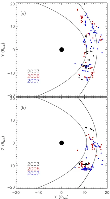
Fig. 1. HFA locations(a)in XY GSE and(b)XZ GSE plane pro-jections and the average bow shock and magnetopause positions. The coordinates were plotted in units ofREarth. The shapes of the magnetopause and the bow shock were calculated with the average solar wind pressure (Sibeck et al., 1991; Tsyganenko, 1995) and Alfv´en-Mach number during HFA formation (Peredo et al., 1995). The black, red and blue points show Cluster positions when HFAs were observed in 2003, 2006 and 2007, respectively.
database of known events since previous analysis was based on significantly fewer events (Schwartz et al., 2000). Our re-sults confirm the rere-sults of Lin (2002) that the size depends on the shear and on the angle between the discontinuity nor-mal and Sun-Earth direction as well; furthermore these re-sults strongly support the recently suggested new condition of HFA formation namely that during HFA formation the typ-ical value of the solar wind speed is higher than the average
(Facsk´o et al., 2008). We have used part of Schwartz et al. (2000)’s calculations so we have checked his formula (Eq. 2) too. Finally the original purpose led us to confirm the find-ings of three different previous theories and to discover sev-eral new independent condition of HFA formation.
The structure of this paper is as follows: we first describe the observational methods and the observed events in Sects. 2 and 3, discuss and present our analysis methods in Sect. 4, and explain and summarize the result of our study in Sect. 5.
2 Data sets
For our study we used 1 s and(22.5 Hz)−1temporal resolu-tion Cluster FGM (Fluxgate Magnetometer) magnetic field data (Balogh et al., 2001) and spin averaged time resolu-tion CIS (Cluster Ion Spectrometry) HIA (Hot Ion Analyzer) plasma measurement data (R`eme et al., 2001). We often found the magnetic signatures of the TD – which interacts with the bow shock and generates the HFA later – in ACE (Advanced Composition Explorer) MAG (Magnetometer In-strument) 16 s temporal resolution magnetic field data se-ries (Smith et al., 1998). Alfv´en Mach numbers were calcu-lated and solar wind velocity was determined based on ACE SWEPAM (Solar Wind Electron, Proton, and Alpha Moni-tor) 16 s temporal resolution data (McComas et al., 1998). ACE SWEPAM data series were used instead of Cluster CIS HIA prime parameter data because in the case of very cold plasmas, as in the solar wind, where thermal velocities are very small compared to the plasma bulk velocity and to the instrument intrinsic energy (and thus velocity) resolution, the relative error in temperature can be large (R`eme et al., 2001; CIS Team, 1997–present); furthermore not all the necessary CIS HIA data has been uploaded onto the Cluster Active Archive yet.
We set a series of criteria for the selection of HFA events based on Thomsen et al. (1986, 1993); Sibeck et al. (1999, 2002) that were:
1. The rim of the cavity must be visible as a sudden in-crease of magnetic field magnitude compared to the un-perturbed solar wind region’s value. Inside the cavity the magnetic field strength drops and its direction turns around.
2. The solar wind speed drops and its direction always turns away from the Sun-Earth direction.
3. The solar wind temperature increases and its value reaches up to several ten million Kelvin degrees. 4. The solar wind particle density also increases on the rim
of the cavity and drops inside the HFA.
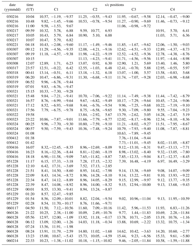
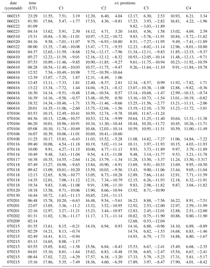
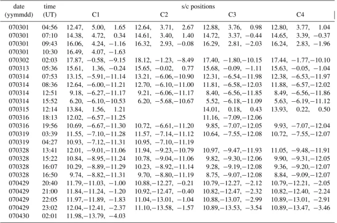
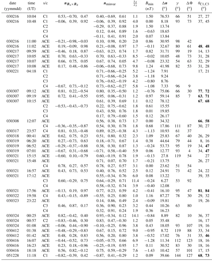
Table 1.The list of studied HFA events and spacecraft positions where HFA was observed in GSE system, inREarthunits. An empty cell indicates that the satellite in question did not observe the magnetic signature of a HFA.
date time s/c positions
(yymmdd) (UT) C1 C2 C3 C4
030216 10:04 10.57, −1.19, −9.57 11.25, −0.55, −9.43 11.95, −0.67, −9.58 12.14, −0.47, −9.00 030216 10:48 9.82, −1.45, −9.66 10.53, −0.78, −9.54 11.27, −0.90, −9.69 11.46, −0.73, −9.12
030216 11:00 9.58, −1.53, 9.67 11.06, −0.98, −9.72
030217 09:59 10.32, 5.78, 6.88 9.59, 10.77, 6.93 10.91, 5.70, 6.41
030217 10:05 10.43, 5.79, 6.84 10.90, 5.10, 6.88 11.03, 5.71, 6.36
030217 10:07 10.47, 5.79, 6.82
030221 04:18 10.43, −2.08, −9.60 11.17, −1.49, −9.46 11.85, −1.67, −9.62 12.06, −1.50, −9.03 030307 09:12 11.29, −4.56, −9.35 12.08, −4.21, −9.16 12.62, −4.51, −9.33 12.89, −4.37, −8.73 030307 09:19 11.18, −4.57, −9.38 11.98, −4.22, −9.19 12.52, −4.52, −9.36 12.78, −4.38, −8.76 030307 10:15 11.13, −4.23, −9.41 11.71, −4.56, −9.56 11.97, −4.44, −8.98 030308 12:07 12.89, 1.71, 6.23 13.07, 0.92, 6.30 12.90, 1.21, 5.69 13.40, 1.46, 5.80 030317 23:57 12.51, −0.22, 6.42 12.55, −1.03, 6.48 12.41, −0.70, 5.88 12.95, −0.55, 5.97 030318 00:41 13.14, −0.51, 6.11 13.18, −1.32, 6.18 13.07, −1.00, 5.57 13.58, −0.83, 5.68 030319 06:20 10.47, −6.86, −9.31 11.30, −6.68, −9.11 11.74, −7.07, −9.28 12.03, −6.98, −8.68 030319 06:52 9.96, −6.78, −9.44
030319 07:01 9.83, −6.76, −9.47 030321 15:15 10.33, −7.30, −9.28
030321 15:48 9.84, −7.21, −9.41 10.70, −7.06, −9.22 11.14, −7.49, −9.38 11.44, −7.42, −8.79 030321 16:57 8.76, −6.99, −9.64 9.67, −6.82, −9.49 10.17, −7.29, −9.64 10.45, −7.24, −9.06 030321 17:12 8.52, −6.93, −9.68 9.44, −6.76, −9.54 9.96, −7.25, −9.68 10.22, −7.19, −9.10 030321 17:56 7.79, −6.75, −9.78 8.75, −6.58, −9.65 9.30, −7.09, −9.80 9.55, −7.04, −9.23 030322 19:58 13.84, −2.92, 5.67 13.79, −2.62, 5.05 14.28, −2.47, 5.19 030323 23:22 10.86, −7.87, −9.01 11.66, −7.79, −8.77 12.02, −8.17, −8.96 12.34, −8.10, −8.36 030324 00:25 9.96, −7.70, −9.30 10.80, −7.59, −9.10 11.21, −8.02, −9.27 11.51, −7.95, −8.67 030324 00:57 9.50, −7.59, −9.43 10.36, −7.48, −9.24 10.79, −7.93, −9.40 11.08, −7.87, −8.81
030324 01:08 10.63, −7.89, −9.45
030412 01:38 7.76,−11.04, −9.44
030412 01:42 7.73,−11.01, −9.45 8.02,−11.05, −8.87
030416 16:07 8.32,−12.45, −8.35 8.96,−12.69, −8.09 9.12,−13.10, −8.31 9.47,−13.13, −7.71 030416 16:23 8.16,−12.36, −8.44 8.81,−12.60, −8.19 8.98,−13.02, −8.40 9.32,−13.05, −7.80 030416 18:18 6.90,−11.58, −9.09 7.65,−11.82, −8.87 7.85,−12.33, −9.04 8.17,−12.37, −8.45 051228 11:17 6.15, 17.33, −3.18 7.28, 17.15, −2.32 7.39, 16.48, −4.19 6.97, 16.49, −3.29 051228 12:10 6.42, 17.31, −3.69 7.52, 17.13, −2.85
051228 21:51 8.41, 14.50, −8.60 8.95, 14.42, −7.98 9.14, 13.38, −9.69 9.08, 14.07, −9.09 051228 22:09 8.43, 14.34, −8.72 8.96, 14.28, −8.10 9.14, 13.22, −9.81 9.10, 13.93, −9.22 051228 22:34 8.47, 14.12, −8.89 8.96, 14.05, −8.29 9.15, 12.99, −9.97 9.12, 13.77, −9.35 051228 22:39 8.47, 14.08, −8.92 8.96, 14.00, −8.32 9.15, 12.94,−10.00 9.13, 13.68, −9.43 051229 00:01 8.55, 13.30, −9.41 8.94, 13.24, −8.87
051229 01:20 8.57, 12.47, −9.85
051229 01:54 8.56, 12.09,−10.01 8.82, 12.04, −9.54 9.02, 10.96,−11.04 9.13, 11.95,−10.59 051229 02:28 8.54, 11.70,−10.17 8.76, 11.66, −9.71
060117 04:50 11.50, 7.12,−10.56 11.60, 7.09,−10.16 11.42, 5.96,−11.53 11.93, 6.83,−11.26 060126 21:22 10.25, 2.38,−11.00 10.09, 2.49,−10.76 9.77, 1.44,−11.83 10.69, 2.28,−11.84 060128 05:56 12.97, 12.00, −1.09 13.92, 11.18, −0.17 13.78, 10.71, −2.05 13.19, 10.76, −1.16 060128 06:12 13.09, 12.00, −1.26 14.03, 11.18, −0.34 13.88, 10.69, −2.22 13.32, 10.75, −1.34 060128 07:24 13.56, 11.91, −1.98
Table 1.Continued.
date time s/c positions
(yymmdd) (UT) C1 C2 C3 C4
060215 23:29 11.55, 7.51, 3.19 12.20, 6.40, 4.04 12.17, 6.30, 2.53 10.93, 6.21, 3.34 060221 01:50 17.04, 5.47, −1.77 17.53, 4.36, −0.81 17.23, 3.93, −2.82 16.81, 4.22, −1.96
060222 01:09 9.82, −3.03,−11.89
060223 04:14 13.62, 5.91, 2.30 14.12, 4.71, 3.20 14.03, 4.56, 1.58 13.02, 4.69, 2.39 060310 15:31 10.84, −5.30,−11.01 10.97, −5.22,−10.72 9.83, −5.76,−11.91 10.84, −5.72,−11.82 060320 04:16 9.58, −7.01,−11.07 9.75, −6.93,−10.80 8.51, −7.27,−11.95 9.49, −7.41,−11.89 060322 08:00 13.35, −7.40,−10.08 13.47, −7.71, −9.55 12.23, −8.02,−11.14 12.96, −8.01,−10.80 060410 04:37 12.65,−11.59, −8.68 12.54,−12.17, −7.96 11.34,−12.11, −9.83 11.85,−12.15, −9.37 060410 05:27 12.23,−11.59, −9.01 12.16,−12.12, −8.32 10.93,−12.05,−10.14 11.48,−12.13, −9.71 060410 07:53 10.89,−11.46, −9.85 10.90,−11.85, −9.27 9.61,−11.75,−10.94 10.23,−11.92,−10.59 060410 08:28 10.54,−11.40,−10.03 10.57,−11.75, −9.47 9.26,−11.64,−11.10 9.91,−11.84,−10.78 060410 12:52 7.54,−10.49,−10.98 7.72,−10.59,−10.64
060416 12:39 13.07, −7.25, 1.87 12.31, −8.49, 1.06
060416 12:45 13.11, −7.33, 1.81 12.40, −8.37, 2.81 12.34, −8.57, 0.99 11.92, −7.82, 1.71 060416 13:22 13.34, −7.72, 1.44 14.04, −9.21, −0.12 13.07,−10.38, −1.08 12.88, −9.82, −0.36 060416 16:30 14.14, −9.51, −0.48 13.46,−10.54, 0.57 13.14,−10.68, −1.47 12.99,−10.13, −0.74 060416 16:39 14.16, −9.58, −0.57 13.48,−10.59, 0.50 13.16,−10.73, −1.54 13.01,−10.19, −0.82 060416 18:32 14.34,−10.46, −1.71 13.70,−11.46, −0.66 13.25,−11.56, −2.77 13.21,−11.11, −2.06 060416 20:01 14.35,−11.06, −2.60 13.75,−12.04, −1.56 13.19,−12.10, −3.70 13.23,−11.72, −3.01 070104 03:53 10.15, 12.49,−10.41 10.59, 12.74, −9.78 10.69, 11.67,−11.24
070104 04:36 10.13, 12.06,−10.57 10.53, 12.34, −9.99 10.64, 11.25,−11.40 10.64, 11.31,−11.38 070104 06:20 10.01, 10.96,−10.91 10.34, 11.30,−10.44 10.44, 10.20,−11.72 10.45, 10.26,−11.71 070104 05:08 10.10, 11.74,−10.69 10.48, 12.03,−10.14 10.59, 10.95,−11.51 10.59, 11.00,−11.49 070106 16:07 10.39, 10.06,−11.01 10.69, 10.41,−10.60
070108 11:25 10.17, 15.81, −6.43 11.03, 15.52, −5.28 11.08, 14.82, −7.27 11.06, 14.84, −7.22 070116 09:40 10.08, 4.54,−11.18 10.19, 5.02,−11.14 10.11, 3.97,−11.93 10.15, 4.03,−11.93 070116 10:00 9.91, 4.27,−11.15 10.00, 4.77,−11.13 9.93, 3.73,−11.89 9.97, 3.79,−11.89 070116 10:49 9.48, 3.63,−11.04 9.54, 4.15,−11.08 9.48, 3.14,−11.77 9.53, 3.21,−11.78 070117 16:38 10.35, 14.55, −2.64 11.24, 13.79, −1.34 11.28, 13.50, −3.37 11.24, 13.50,−3.317 070118 07:49 13.27, 10.98, −9.65 13.84, 10.90, −8.91 13.69, 9.91,−10.53 13.69, 9.95,−10.50 070118 09:42 13.09, 10.01,−10.20 13.59, 10.03, −9.56 13.43, 9.00,−11.06 13.44, 9.05,−11.04 070118 12:13 12.65, 8.58,−10.77 13.05, 8.73,−10.28 12.89, 7.66,−11.61 12.91, 7.71,−11.59 070118 14:35 12.01, 7.08,−11.12 12.31, 7.34,−10.79 12.15, 6.26,−11.93 12.18, 6.32,−11.91 070118 19:34 9.83, 3.48,−11.08 9.91, 3.98,−11.10 9.83, 2.98,−11.82 9.87, 3.04,−11.82 070120 18:18 13.58, 9.71,−10.06 13.90, 8.66,−10.94 13.92, 8.71,−10.90
070130 16:44 10.72, 1.63,−11.13 10.85, 2.01,−11.13
070201 06:48 15.78, 10.20, −6.63 16.48, 9.54, −5.61 16.23, 8.88, −7.56 16.22, 8.91, −7.51 070201 22:07 13.05, 3.36, −11.2 13.32, 3.52,−10.95 12.92, 2.53,−12.00 12.97, 2.59,−11.99 070201 22:16 12.97, 3.27,−11.21 13.23, 3.44,−10.97 12.83, 2.45,−12.01 12.88, 2.51,−12.00 070202 01:31 11.02, 1.36,−11.17 11.17, 1.71,−11.14 10.82, 0.75,−11.90 10.88, 0.80,−11.90
070209 02:14 12.68, 0.53,−12.04
070215 01:35 13.61, 8.15, −0.21 14.10, 6.94, 0.93 14.16, 6.88, −0.96 14.10, 6.89, −0.89 070215 02:29 14.21, 8.13, −0.74 14.74, 6.82, −1.53 14.68, 6.83, −1.46 070215 02:49 14.41, 8.11, −0.94 14.93, 6.79, −1.73 14.88, 6.80, −1.67 070215 03:13 14.65, 8.08, −1.17
Table 1.Continued.
date time s/c positions
(yymmdd) (UT) C1 C2 C3 C4
070301 04:56 12.47, 5.00, 1.65 12.64, 3.71, 2.67 12.88, 3.76, 0.98 12.80, 3.77, 1.04 070301 07:10 14.38, 4.72, 0.34 14.61, 3.40, 1.40 14.72, 3.37, −0.44 14.65, 3.39, −0.37 070301 09:43 16.06, 4.24, −1.16 16.32, 2.93, −0.08 16.29, 2.81, −2.03 16.24, 2.83, −1.96 070301 10:30 16.49, 4.07, −1.63
070302 02:03 17.87, −0.58, −9.15 18.12, −1.23, −8.49 17.40, −1.80,−10.15 17.44, −1.77,−10.10 070313 05:36 15.61, 1.36, −0.24 15.65, −0.02, 0.77 15.68, −0.09, −1.11 15.63, −0.05, −1.04 070314 07:53 13.15, −5.91,−11.14 13.21, −6.06,−10.90 12.31, −6.54,−11.98 12.38, −6.53,−11.97 070314 08:36 12.64, −6.00,−11.21 12.70, −6.10,−11.00 11.81, −6.58,−12.03 11.88, −6.57,−12.02 070314 12:51 9.18, −6.27,−11.17 9.21, −6.06,−11.17 8.40, −6.56,−11.85 8.49, −6.56,−11.86 070314 15:52 6.20, −6.10,−10.53 6.20, −5.68,−10.67 5.52, −6.18,−11.09 5.63, −6.19,−11.12
070315 12:14 13.84, 1.56, 1.21 14.01, 0.18, 0.43 13.93, 0.22, 0.50
070316 18:13 12.02, −6.57,−11.25 11.16, −7.09,−12.06
070316 19:56 10.69, −6.67,−11.30 10.72, −6.61,−11.20 9.85, −7.07,−12.05 9.93, −7.07,−12.04 070319 03:39 11.55, −7.10,−11.28 11.57, −7.14,−11.12 10.64, −7.55,−12.08 10.72, −7.55,−12.07 070319 04:27 10.93, −7.12,−11.31 10.95, −7.10,−11.19
070328 13:41 12.01, −9.01,−11.06 11.94, −9.23,−10.79 10.97, −9.47,−11.93 11.05, −9.48,−11.91 070328 15:22 10.84, −8.95,−11.24 10.78, −9.04,−11.06 9.82, −9.30,−12.06 9.90, −9.31,−12.05 070328 16:07 10.29, −8.89,−11.29 10.23, −8.92,−11.14 9.28, −9.19,−12.08 9.36, −9.20,−12.07 070328 16:50 9.74, −8.82,−11.31 9.70, −8.80,−11.19 8.75, −9.07,−12.08 8.84, −9.09,−12.07 070429 20:40 11.79,−11.03, −1.00 10.88,−12.27, −0.21 10.79,−12.27, −2.12 10.79,−12.21, −2.05 070429 21:00 11.84,−11.24, −1.20 10.92,−12.47, −0.40 10.82,−12.47, −2.32 10.82,−12.40, −2.24 070429 22:05 11.97,−11.89, −1.83 11.04,−13.01, −1.04 10.88,−13.07, −2.99 10.89,−13.01, −2.91 070429 23:02 12.04,−12.41, −2.37 11.10,−13.58, −1.57 10.89,−13.53, −3.54 10.89,−13.47, −3.46 070430 02:01 11.98,−13.79, −4.03
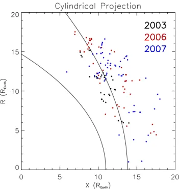
in the 2003 data was analyzed by Facsk´o et al. (2008). The positions of the events are given in Table 1 and Fig. 1. All of them were observed beyond the bow shock in the February– April 2003, December 2005–April 2006 and January–April 2007 time intervals. A fraction of these events was located very far from the bow shock and the Earth (≥19REarth), oc-curring mainly in 2007. Only the position of tetrahedron center of the Cluster SC is plotted in Figs. 1, 2 because the length of the orbital section is comparable with the thickness of the lines drawn. The bow shock position was calculated using the average Alfv´en Mach number during formation of the events (MA=11.8, Sect. 3.2) according to the model de-scribed in Peredo et al. (1995). The position of the magne-topause was calculated using the same average solar wind pressure (1.73±0.8 nPa, Sect. 3.3) as that in Sibeck et al. (1991) and Tsyganenko (1995).
The cylindrical projection of the center of the Cluster SC positions is also plotted to more easily determine whether the observations were performed beyond or inside the average bow shock (Fig. 2). Figure 1 seems to indicate that the HFAs are mostly located within the magnetosheath, with some in-side the magnetosphere. However, this is only a feature of the applied projection. The position of the bow shock was calculated using the average solar wind pressure during, the HFA event. All HFAs were beyond the actual bow shock when we observed them. However the bow shock position
changes quickly, presenting explanation for why some of the events seem to be located in the magnetosheath.
3 Analysis
3.1 Size-angle plots
The main purpose of this paper is to determine experimen-tally the role the different angles (γ,18) play in controlling HFA size. In the next two sections we therefore calculate the angles associated with each HFA and its size.
3.1.1 Determination of angles
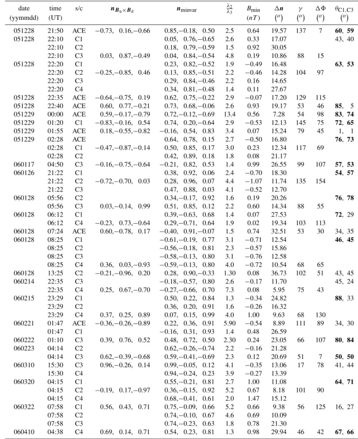
Table 2.Parameters of TD normal vectors:λ2/λ3is the ratio of 2nd and 3rd eigenvalues,Bminis the smallest magnetic field component in
minimum variance system,1nis the error cone of minimum variance method,γis the angle between the Sun direction and TD normal,18
is the direction change across the discontinuity andθthe angle between the bow shock normal and theBmagnetic field vector. Boldface
letter shows quasi-perpendicular conditions; the angles were calculated by scaling a model BS to the location of Cluster-1 and 3 spacecraft.
date time s/c nB
u×Bd nminvar
λ2
λ3 Bmin 1
n γ 18 θC1,C3
(yymmdd) (UT) (nT ) o o o o
030216 10:04 C1 0.53,−0.70, 0.47 0.40,−0.69, 0.61 1.1 1.50 76.53 66 51 27, 27 030216 10:48 C1 −0.06, 0.39, 0.92 −0.06, 0.39, 0.92 4.0 0.00 8.18 93 73 37, 45
C2 −0.29, 0.37, 0.88 1.9 1.50 13.74
C3 0.12, 0.44, 0.89 1.6 −0.63 18.65
C4 −0.11, 0.41, 0.91 2.0 0.07 13.84
030216 11:00 ACE −0.21,−0.98,−0.03 0.10, 0.98, 0.20 2.0 0.86 30.95 98 42
030216 11:02 ACE 0.19,−0.09, 0.98 0.21,−0.08, 0.97 1.7 −0.11 32.67 80 61 48, 48
030217 09:59 ACE −0.46, 0.18, 0.87 −0.63, 0.23, 0.74 1.7 0.82 31.71 99 19 14, 13 030217 10:05 ACE 0.70, 0.63,−0.33 0.70, 0.63,−0.33 8.5 −0.02 10.05 48 73 31, 28 030217 10:07 ACE 0.66, 0.75, 0.05 0.67, 0.74, 0.05 4.7 −0.08 23.32 54 63 32, 29 030217 10:08 ACE 0.17, 0.48,−0.86 −0.06,−0.68, 0.73 9.8 1.24 41.98 82 53 31, 28
030221 04:18 C1 0.71,−0.66,−0.25 5.2 −1.24 7.91 17, 21
C2 0.71,−0.66,−0.24 3.8 −1.18 9.24
C3 0.76,−0.62,−0.19 4.2 −0.80 8.76
C4 −0.67, 0.73,−0.12 0.73,−0.62,−0.27 5.8 −1.08 7.33 96 9
030307 09:12 ACE 0.81, 0.22,−0.54 0.80, 0.35,−0.50 1.2 −0.76 75.06 66 30 77, 72
030307 09:19 ACE 0.72, 0.41,−0.55 0.95, 0.06,−0.31 1.2 0.97 59.14 85 7 63, 71
030307 10:15 ACE 0.61, 0.39, 0.69 1.1 0.12 78.12 67, 68
C2 −0.53,−0.43,−0.73 0.22, 0.75,−0.62 1.8 0.61 15.55
C3 0.43, 0.50, 0.76 1.8 0.01 19.85
C4 0.17, 0.79,−0.60 1.5 0.12 26.17
030308 12:07 ACE 0.56, 0.38, 0.73 1.7 0.00 34.32 66, 58
C4 −0.36,−0.35,−0.87 0.54, 0.30, 0.78 1.8 0.68 17.86 111 87 30, 27 030317 23:57 C4 0.81, 0.33,−0.48 0.89, 0.25,−0.38 4.3 −1.13 10.93 61 37
030318 00:41 ACE 0.62, 0.75, 0.23 0.51, 0.80, 0.32 2.3 1.09 25.83 67 40 26, 29 030319 06:20 ACE 0.27,−0.73, 0.63 0.18,−0.71, 0.67 1.4 0.38 44.64 79 44 8, 16 030319 06:52 ACE −0.29,−0.37,−0.88 0.38, 0.30, 0.87 1.3 −0.24 53.73 95 19 34, 47
030319 07:01 ACE −0.67, 0.31,−0.68 −0.71, 0.58,−0.40 5.9 0.06 12.77 93 4 34, 47
030321 15:15 ACE −0.60, 0.10,−0.79 0.60,−0.19, 0.78 1.9 −0.13 27.8 119 54 27
030321 15:48 ACE 0.71, 0.07, 0.70 1.7 −0.21 13.75 26, 27
C4 0.78, 0.27, 0.57 0.78, 0.27, 0.57 3.1 0.00 23.62 51 54
030321 16:57 ACE 0.43, 0.73, 0.53 0.40, 0.76, 0.52 2.5 0.12 24.91 73 42 24, 22
030321 17:12 ACE 0.55,−0.34, 0.76 6.0 0.08 13.22 39, 35
C3 0.60,−0.29, 0.75 0.64,−0.29, 0.71 11.4 −0.24 6.27 53 92
C4 0.58,−0.32, 0.74 3.9 −0.40 12.08
030321 17:56 ACE −0.13, 0.19, 0.97 0.77, 0.23, 0.59 4.2 −0.41 16.10 95 47 81, 84
030322 19:58 C4 0.43,−0.15, -0.89 −0.55, 0.25, 0.80 1.0 1.16 87.27 78 30 29, 32
030323 23:22 ACE 0.14, 0.86, 0.49 2.4 −0.09 19.81 19, 26
C3 0.46, 0.87, 0.17 0.36, 0.90, 0.23 3.2 0.44 10.26 63 80
C4 0.32, 0.91, 0.24 1.9 0.36 16.23
030324 00:25 ACE 0.82,−0.42, 0.40 0.93,−0.34, 0.12 14.1 −0.84 8.89 82 10 36, 37 030324 00:57 C2 −0.83,−0.46, 0.30 0.83, 0.47,−0.30 1.2 0.05 35.48 16, 17 030324 01:08 ACE −0.06, 0.44,−0.90 −0.10,−0.25, 0.96 3.8 0.43 18.05 93 107 19, 16 030412 01:38 ACE −0.48,−0.29,−0.83 0.67, 0.15, 0.72 9.0 −0.95 8.72 119 88 33, 34 030412 01:42 ACE 0.48, 0.28, 0.83 0.56, 0.20, 0.80 3.8 −0.52 17.02 76 31 35, 46
Table 2.Continued.
date time s/c nB
u×Bd nminvar
λ2
λ3 Bmin 1
n γ 18 θC1,C3
(yymmdd) (UT) (nT ) o o o o
051228 21:50 ACE −0.73, 0.16,−0.66 0.85,−0.18, 0.50 2.5 0.64 19.57 137 7 60, 59
051228 22:10 C1 0.05, 0.76,−0.65 2.6 0.33 17.07 43, 40
22:10 C2 0.18, 0.79,−0.59 1.5 0.92 30.05
22:10 C3 0.03, 0.87,−0.49 0.04, 0.84,−0.54 4.8 0.19 10.86 88 15
051228 22:20 C1 0.23, 0.82,−0.52 1.9 −0.49 16.48 63, 53
22:20 C2 −0.25,−0.85, 0.46 0.13, 0.85,−0.51 2.2 −0.46 14.28 104 97
22:20 C3 0.29, 0.84,−0.46 2.2 0.16 14.65
22:20 C4 0.34, 0.81,−0.48 1.4 0.11 27.67
051228 22:35 ACE −0.64,−0.75, 0.19 0.62, 0.75,−0.22 2.9 −0.07 17.20 129 115
051228 22:40 ACE 0.60, 0.77,−0.21 0.73, 0.68,−0.06 2.6 0.93 19.17 53 46 85, 5 051229 00:00 ACE 0.59,−0.17,−0.79 0.72,−0.12,−0.69 13.4 0.56 7.28 54 98 83, 74
051229 01:20 C1 −0.83,−0.16, 0.54 0.74, 0.20,−0.64 2.9 −0.53 12.13 145 75 72, 65
051229 01:55 ACE 0.18,−0.55,−0.82 −0.16, 0.54, 0.83 3.4 0.07 15.24 79 45 1, 1
051229 02:28 ACE 0.64, 0.78, 0.15 2.7 −0.50 16.80 76, 73
02:28 C1 −0.47,−0.87,−0.14 0.50, 0.85, 0.17 3.0 0.23 12.34 117 69
02:28 C2 0.42, 0.89, 0.18 1.8 0.08 21.17
060117 04:50 C3 −0.16,−0.75,−0.64 −0.21, 0.82, 0.53 1.4 0.99 26.55 99 107 57, 53
060126 21:22 C1 0.38, 0.92, 0.06 2.4 −0.70 18.30 54, 57
21:22 C2 −0.72,−0.70, 0.03 0.28, 0.96, 0.07 4.4 −1.07 11.74 135 154
21:22 C3 0.47, 0.88, 0.03 4.1 −0.52 12.70
060128 05:56 C2 0.34,−0.17, 0.92 1.6 0.19 20.26 76, 78
05:56 C3 0.03,−0.14, 0.99 0.51, 0.85, 0.12 2.2 0.60 14.34 88 55
060128 06:12 C1 0.39,−0.63, 0.68 1.4 0.07 27.53 72, 29
06:12 C4 −0.23, 0.73,−0.64 0.29,−0.71, 0.64 1.9 0.02 19.34 103 113
060128 07:24 ACE 0.60,−0.78, 0.17 −0.40, 0.91,−0.07 1.5 0.74 32.51 53 30 34, 35
060128 08:25 C1 −0.61,−0.19, 0.77 3.1 −0.71 12.54 46, 45
08:25 C2 −0.56,−0.18, 0.81 2.3 −0.57 15.86
08:25 C3 −0.58,−0.13, 0.80 3.1 −0.76 12.58
08:25 C4 0.36, 0.03,−0.93 −0.59,−0.13, 0.80 4.0 −0.72 10.54 68 65
060128 13:25 C2 −0.21,−0.96, 0.20 0.28, 0.90,−0.33 1.30 0.08 36.73 102 51 43, 45
060214 22:35 C3 −0.18,−0.57, 0.80 2.6 −0.17 11.70 45, 24
22:35 C4 0.25, 0.67,−0.70 −0.27,−0.66, 0.70 7.3 0.08 5.95 75 43
060215 23:29 C1 0.50, 0.22, 0.84 1.3 −0.34 24.82 88, 33
23:29 C2 0.36, 0.20, 0.91 1.6 −0.26 16.32
23:29 C4 0.37, 0.25, 0.89 0.07, 0.15, 0.99 4.0 1.00 9.63 68 130
060221 01:47 ACE −0.36,−0.26,−0.89 0.22, 0.36, 0.91 5.90 −0.54 8.89 111 89 34, 30
01:47 C1 −0.16, 0.31, 0.93 1.4 0.48 26.59
060222 01:10 C3 0.39, 0.76, 0.52 0.48, 0.72, 0.50 2.30 0.24 23.05 66 107 80, 84
060223 04:14 C2 0.62,−0.26,−0.74 2.2 −0.16 21.28
04:14 C3 0.62,−0.39,−0.68 0.59,−0.41,−0.69 2.3 0.12 20.69 51 7 50, 50
060310 15:30 C3 0.96,−0.26, 0.14 0.99,−0.05, 0.12 4.1 −0.35 13.06 17 78 41, 44
15:30 C4 0.94,−0.24, 0.23 3.9 −0.27 13.39
060320 04:15 C1 0.55,−0.21, 0.81 2.7 1.00 11.08 64, 71
04:15 C2 −0.19, 0.17,−0.97 0.36,−0.15, 0.92 5.2 0.67 8.18 101 90
04:15 C4 0.68,−0.41, 0.61 2.0 1.47 15.12
060322 07:58 C1 0.56, 0.43, 0.71 0.75,−0.09, 0.66 5.2 0.66 9.38 56 125 16, 27
07:58 C2 0.74,−0.10, 0.67 4.6 0.69 10.09
07:58 C3 0.74,−0.23, 0.63 1.8 0.78 21.30
Table 2.Continued.
date time s/c nB
u×Bd nminvar
λ2
λ3 Bmin 1
n γ 18 θC1,C3
(yymmdd) (UT) (nT ) o o o o
060410 05:28 C1 0.66, 0.39, 0.64 1.4 −0.96 35.69 41, 43
05:28 C3 0.53, 0.56, 0.64 0.49, 0.59, 0.64 1.7 0.15 27.49 58 116
05:28 C4 0.46, 0.57, 0.68 1.4 −0.55 39.17
060410 07:53 C2 0.60, 0.18, 0.78 0.76, 0.16, 0.63 2.3 −0.83 15.52 53 42 32, 32
07:53 C4 0.62,−0.08, 0.78 1.9 −1.01 20.03
060410 08:30 C1 0.84,−0.01, 0.55 1.1 −1.03 43.56 30, 34
08:30 C2 0.80, 0.07, 0.60 3.7 −0.72 11.81
08:30 C3 0.62, 0.39, 0.68 0.76, 0.13, 0.64 4.9 −0.62 9.79 51 114
08:30 C4 0.76, 0.11, 0.64 4.7 −0.67 9.95
060410 12:52 C1 −0.15,−0.12, 0.98 −0.57, 0.05, 0.82 2.6 1.59 15.89 98 17 81, 81
12:52 C2 0.84, 0.18,−0.51 1.7 −0.85 24.58
060416 12:38 C2 −0.37, 0.23, 0.90 0.49, 0.75, 0.43 1.3 −0.07 28.76 112 8 39, 60
060416 12:45 C1 −0.06,−0.69,−0.72 −0.09, 0.77, 0.63 5.4 −0.75 11.20 93 36
12:45 C2 0.09, 0.73, 0.68 2.1 0.46 22.20
060416 13:24 C1 0.77, 0.54, 0.33 0.73, 0.36, 0.58 1.5 0.30 35.29 39 36
060416 15:56 C4 0.23,−0.59, 0.77 0.44,−0.26, 0.86 6.4 −0.38 7.77 76 25 48, 47
060416 16:29 C1 0.31, 0.63, 0.71 6.0 0.52 9.24 43, 54
16:29 C2 0.01,−0.81,−0.58 0.14, 0.75, 0.65 14.4 0.30 5.63 89 126
060416 16:40 ACE −0.78,−0.37,−0.51 0.85, 0.12, 0.52 1.7 0.44 20.40 140 109 43, 54
16:40 C1 0.83,−0.08,−0.55 1.4 −0.11 29.50
060416 18:33 ACE 0.30,−0.09,−0.95 −0.48,−0.17, 0.86 3.5 −0.35 12.03 72 22 44, 49
060416 20:01 C3 −0.05, 0.29, 0.96 0.17, 0.44, 0.88 2.0 −0.03 14.97 92 10 49, 48
20:01 C4 0.29, 0.43, 0.85 1.5 −0.20 21.62
070104 03:54 C2 0.83,−0.33, 0.45 0.25, 0.93, 0.29 1.3 −0.50 32.78 33 27 44, 44 070104 04:38 ACE −0.63, 0.64,−0.45 0.68,−0.72, 0.13 10.3 −1.48 7.73 128 26 31, 31
070104 05:08 ACE 0.60,−0.54, 0.58 2.2 −0.03 19.08
05:08 C1 0.71,−0.61, 0.35 2.9 −0.16 14.68
05:08 C2 0.57,−0.68, 0.46 2.1 0.12 19.78
05:08 C3 0.64,−0.64, 0.43 0.68,−0.62, 0.40 3.0 −0.15 13.51 50 113
05:08 C4 0.58,−0.67, 0.46 2.6 0.10 16.49
070104 06:20 ACE 0.62, 0.04, 0.78 0.61, 0.05, 0.79 7.1 0.04 8.63 51 96 23, 23
06:20 C1 0.73, 0.30, 0.62 1.8 −0.05 20.18
070106 16:10 C1 0.24, 0.44, 0.86 0.21, 0.76, 0.61 1.7 0.66 20.21 75 8 10, 5
070108 11:25 ACE −0.51, 0.86,−0.01 2.2 0.03 17.13 82, 74
11:25 C1 −0.62, 0.78, 0.01 −0.66, 0.75, 0.02 2.4 −0.04 12.24 128 129
11:25 C2 −0.67, 0.74, 0.06 2.1 −0.05 15.71
11:25 C3 −0.50, 0.86,−0.06 1.2 0.04 37.42
11:25 C4 0.50,−0.86, 0.05 1.3 −0.08 30.75
070116 09:41 C1 0.36, 0.29, 0.88 0.36, 0.17, 0.92 2.3 −0.37 14.57 68 6 24, 22 070116 10:00 ACE 0.98,−0.11, 0.15 0.94,−0.29,−0.17 2.2 0.25 17.96 10 160 21, 16
070116 10:50 C1 0.74,−0.64, 0.20 3.9 −0.12 9.57 28, 28
10:50 C2 0.73,−0.63, 0.26 3.0 −0.11 11.49
10:50 C3 −0.73, 0.61,−0.31 0.68,−0.61, 0.40 4.4 0.22 8.72 136 43
070116 10:50 C4 0.69,−0.62, 0.37 4.4 0.16 8.70
070117 16:40 ACE −0.49,−0.74,−0.46 0.55, 0.55, 0.63 1.9 −0.80 24.59 119 82 9, 12 070118 07:52 C3 0.50, 0.85, 0.14 0.45, 0.88, 0.18 1.5 0.30 25.86 59 57 28, 24
070118 07:52 C4 0.51, 0.85, 0.12 1.1 −0.19 48.52
Table 2.Continued.
date time s/c nB
u×Bd nminvar
λ2
λ3 Bmin 1
n γ 18 θC1,C3
(yymmdd) (UT) (nT ) o o o o
070118 12:15 C1 −0.80,−0.10, 0.59 −0.84, 0.08,−0.53 2.9 −0.18 12.16 143 87 38, 9
070118 14:36 C1 0.07, 1.00,−0.04 2.2 0.03 13.11 36, 14
14:36 C2 0.04, 1.00,−0.02 2.7 0.05 10.83
14:36 C3 −0.02,−1.00, 0.02 0.03, 1.00,−0.15 2.9 −0.60 10.69 91 28
070118 19:35 C1 0.52, 0.79,−0.33 2.7 −0.18 12.26 87, 87
19:35 C2 0.55, 0.77,−0.31 2.1 0.01 14.83
19:35 C3 0.41, 0.80,−0.44 2.4 0.23 13.41
19:35 C4 0.50, 0.77,−0.39 0.46, 0.80,−0.40 3.3 0.10 10.51 60 81
070120 18:20 C1 0.69,−0.40, 0.60 7.2 −0.42 6.28
18:20 C2 0.51,−0.42, 0.75 0.60,−0.41, 0.69 10.3 −0.31 5.19 59 100
18:20 C3 0.61,−0.40, 0.68 8.3 −0.40 5.89
18:20 C4 0.63,−0.41, 0.66 7.6 −0.51 6.14
070130 16:47 ACE 0.67,−0.58, 0.46 0.83,−0.46, 0.31 1.8 −0.80 28.51 47 26 23, 17 070201 06:49 C1 0.24,−0.33, 0.91 0.26,−0.33, 0.91 2.2 −0.07 15.73 75 71 41, 44
06:49 C2 −0.11,−0.39, 0.91 1.0 0.57 104.85
06:49 C3 −0.20,−0.47, 0.86 1.3 0.87 32.17
06:49 C4 −0.11,−0.47, 0.88 1.2 0.66 41.45
070201 22:08 C1 0.30,−0.89, 0.33 −0.35, 0.88,−0.31 3.0 0.05 12.58 72 37 64, 61
22:08 C2 −0.38, 0.90,−0.21 2.6 0.65 13.92
22:08 C3 −0.43, 0.86,−0.29 2.7 0.16 13.66
22:08 C4 −0.42, 0.85,−0.30 1.9 0.16 18.62
070201 22:17 ACE 0.22,−0.89, 0.41 0.15,−0.89, 0.44 16.9 0.16 6.57 77 64 57, 43
22:17 C3 −0.23, 0.84,−0.48 2.1 0.13 21.55
070202 01:31 ACE −0.42, 0.91, 0.02 2.5 0.08 15.51 83, 83
01:31 C1 0.53,−0.84,−0.10 −0.57, 0.80, 0.18 4.0 0.29 9.43 58 25
01:31 C2 −0.44, 0.89, 0.05 3.0 −0.26 12.34
070209 02:16 C1 −0.96,−0.25, 0.14 0.94, 0.29,−0.16 5.8 −0.13 8.62 163 89 72, 63
02:16 C2 0.92, 0.35,−0.19 5.8 −0.16 8.68
070215 01:35 C2 0.31,−0.05,−0.95 −0.38, 0.14, 0.91 2.2 0.31 14.35 71 55 25, 28
070215 02:31 ACE 0.66,−0.21, 0.73 3.0 0.01 13.32 25, 28
02:31 C1 0.72,−0.33, 0.61 0.70,−0.33, 0.63 5.9 0.06 6.73 43 102
02:31 C3 0.55,−0.35, 0.75 1.6 −0.05 19.96
02:31 C4 0.52,−0.37, 0.77 1.7 0.10 15.51
070215 02:50 ACE −0.40,−0.22, 0.89 3.7 −0.11 13.76 25, 28
02:50 C1 0.63,−0.06, 0.77 1.2 −0.14 26.49
02:50 C2 0.14, 0.19,−0.97 0.80, 0.30,−0.53 4.5 −1.09 5.53 82 138
02:50 C3 0.66,−0.17, 0.73 1.6 0.00 16.97
02:50 C4 0.68,−0.17, 0.71 1.4 0.00 19.53
070215 03:13 C1 0.43,−0.27,−0.86 0.70,−0.54,−0.47 1.6 −0.27 24.17 64 8 27, 29 070215 03:56 C4 0.43, 0.31, 0.85 0.66, 0.35, 0.66 9.1 −1.25 6.78 64 100 25, 25 070215 04:00 C1 −0.06,−0.71,−0.70 0.05, 0.75, 0.65 1.9 −0.13 20.13 93 20
070215 08:45 C1 0.82, 0.41, 0.40 0.79, 0.44, 0.42 6.5 −0.08 6.81 35 66 10, 25
08:45 C2 0.84, 0.17, 0.51 2.3 0.10 16.65
08:45 C3 0.75, 0.26, 0.61 1.6 0.18 26.22
08:45 C4 0.70, 0.20, 0.68 1.6 0.29 25.26
070215 15:15 C3 0.45,−0.53, 0.72 0.49,−0.53, 0.69 3.4 −0.14 11.26 63 74 44, 53
070215 15:15 C4 0.48,−0.51, 0.71 2.7 −0.08 13.36
070215 22:08 C2 −0.38, 0.90,−0.21 2.6 0.65 13.92
Table 2.Continued.
date time s/c nB
u×Bd nminvar
λ2
λ3 Bmin 1
n γ 18 θC1,C3
(yymmdd) (UT) (nT ) o o o o
070301 04:56 C3 0.64,−0.77,−0.06 1.2 −0.05 32.86
04:56 C4 0.64,−0.76,−0.11 1.2 0.07 35.48
070301 07:11 C1 0.97,−0.13, 0.20 2.2 -0.15 12.07 20, 21
07:11 C2 −0.93, 0.16,−0.33 0.93,−0.15, 0.35 2.9 0.03 9.77 158 99
07:11 C3 0.92,−0.18, 0.34 2.5 −0.08 10.93
070301 09:43 C1 0.47,−0.80,−0.37 1.7 0.21 15.12 87, 89
09:43 C2 0.72,−0.69,−0.03 0.78,−0.60,−0.15 2.0 −0.34 12.93 43 17
070301 10:30 C1 −0.61, 0.64,−0.46 −0.56, 0.79,−0.26 1.9 −0.29 15.42 127 8 16, 23 070302 02:03 C1 0.71, 0.69, 0.12 0.80, 0.57, 0.18 2.1 −0.17 12.71 44 8 47, 51
070313 05:37 C2 0.60, 0.52,−0.61 0.61, 0.52,−0.60 5.2 −0.05 7.48 53 92 24, 23
05:37 C3 0.67, 0.52,−0.53 3.2 −0.53 11.53
05:37 C4 0.69, 0.49,−0.52 3.8 −0.48 10.35
070314 07:54 ACE 0.37, 0.32, 0.87 0.38, 0.29, 0.88 2.9 −0.14 15.87 68 68 39, 39
070314 08:37 C1 0.74, 0.43, 0.52 1.8 0.27 30.34 45, 39
08:37 C3 0.76, 0.31, 0.57 0.77, 0.00, 0.64 4.0 0.08 15.22 40 17
08:37 C4 0.70, 0.20, 0.68 2.9 0.28 18.32
070314 12:51 ACE −0.17, 0.21,−0.96 0.30,−0.50, 0.81 2.0 −0.18 22.90 99 26 51, 51
070314 15:52 ACE −0.85,−0.46,−0.26 0.86, 0.52,−0.03 1.9 0.16 21.58 147 163 9, 9 070315 12:15 ACE 0.40,−0.23, 0.89 0.48,−0.08, 0.87 2.2 0.32 20.23 66 109 58, 58
12:15 C1 0.37,−0.40, 0.84 1.5 −0.07 22.67
070316 18:14 C1 −0.15,−0.98, 0.12 0.17, 0.97,−0.18 2.0 −0.22 14.41 98 12 40, 39
070316 19:57 C1 0.64,−0.61, 0.46 1.6 −0.08 17.19 51, 53
19:57 C2 0.56,−0.53, 0.63 1.6 −0.02 16.57
19:57 C3 0.41,−0.51, 0.75 1.2 0.13 30.65
19:57 C4 0.37,−0.39, 0.84 0.31,−0.50, 0.81 1.7 0.17 16.15 68 38
070319 03:47 C2 0.83, 0.03, 0.56 1.1 −0.04 48.73 49, 30
070319 03:47 C4 0.56, 0.14, 0.82 0.20, 0.19, 0.96 2.1 0.30 14.07 56 144
070319 04:28 C1 0.50, 0.42, 0.76 2.1 −0.14 13.22 16, 13
070319 04:28 C2 0.32, 0.40, 0.86 1.9 0.02 15.32
070319 04:28 C3 −0.24,−0.39,−0.89 0.20, 0.38, 0.90 2.3 0.06 12.42 104 96
070328 13:41 C3 0.90, 0.31, 0.29 0.90, 0.30, 0.30 1.5 −0.01 20.23 25 47 9, 88
13:41 C4 0.86, 0.38, 0.34 1.5 0.11 20.58
070328 15:22 C2 0.23,−0.93,−0.28 −0.24, 0.96,−0.15 1.9 −0.06 24.12 76 4 35, 30 070328 16:08 C2 0.04, 1.00, 0.05 −0.09, 0.95, 0.29 1.4 −0.30 23.79 87 13 36, 47
070328 16:51 C1 0.63,−0.22,−0.74 1.7 0.01 16.24 66, 71
16:51 C2 0.51,−0.24,−0.82 2.0 0.00 13.11
16:51 C4 0.05,−0.15,−0.99 −0.50, 0.28, 0.82 2.4 −0.34 11.23 86 16
070429 20:41 C2 −0.79,−0.55, 0.29 0.79, 0.54,−0.29 2.6 0.04 12.24 141 68 39, 40 070429 21:00 C1 −0.79,−0.48, 0.37 0.72, 0.35,−0.60 1.4 0.66 18.29 142 27 51, 52
070429 22:06 C1 −0.37,−0.90,−0.23 0.33, 0.85, 0.41 1.2 −0.52 27.17 111 44 39, 40 070429 23:02 ACE −0.77, 0.14,−0.63 0.72,−0.11, 0.69 4.9 −0.18 10.03 140 115
23:02 C1 0.66,−0.04, 0.75 1.8 0.14 14.56
23:02 C2 0.72,−0.07, 0.69 1.9 0.26 13.85
23:02 C3 0.65,−0.03, 0.76 2.3 −0.09 11.31
23:02 C4 0.71,−0.03, 0.70 1.9 −0.04 15.05
070430 02:02 C1 −0.23,−0.46,−0.86 0.65, 0.40, 0.64 6.3 0.65 5.92 103 146
02:02 C2 0.67, 0.40, 0.62 5.6 0.70 6.39
02:02 C3 0.68, 0.40, 0.61 5.5 0.48 6.50
Fig. 2. Cylindrical projection of Cluster SC center positions dur-ing HFA observation and the average bow shock and magnetopause positions in GSE system. The shape of the magnetopause and the bow shock were calculated using the average solar wind pressure (Sibeck et al., 1991; Tsyganenko, 1995; Peredo et al., 1995). The black, red and blue points show the Cluster SC positions when HFA was observed in 2003, 2006 and 2007, respectively. The coordinates were plotted inREarthunits.
minimum variance method if the cross product method did not differ by more than 15◦and the ratio of second and third eigenvalues were equal to or larger than 2.0 (Table 2) (for a more detailed description of the method see Facsk´o et al., 2008; Facsk´o et al., 2009). It turns out that the minimum variance method can mostly be used at low magnetic field variation. This method is very difficult and almost impossi-ble to use in the HFA cavity and in SLAMS (Short Large Amplitude Magnetic Structures) mostly coupled to quasi-parallel regions (Schwartz and Burgess, 1991). Many HFAs were embedded into SLAMS and so we were able to use the minimum variance method with good accuracy only in a few cases. Beside of this feature of the method we have found more HFAs at the quasi-parallel region (∼66%) (see Table 2). The local bow shock normals were calculated by scaling a model bow shock to the spacecraft location as in Schwartz et al. (2000) and we used the upstream magnetic field up-stream of the HFA to calculate the angle of the shock-normal and the magnetic field vector. This might confirm previous results: the conditions were quasi-parallel at least on one side of the TD previously (see Onsager et al., 1991; Thomsen et al., 1993; Kecskem´ety et al., 2006) and current simulations expect the HFAs to appear where the quasi-parallel condition turns to quasi-perpendicular (Omidi and Sibeck, 2007). We
Fig. 3.Distribution of cos18where18is the angle of magnetic field directional change at the discontinuity.
used the same conditions for HFA observation and determi-nation in 2003 (Kecskem´ety et al., 2006; Facsk´o et al., 2008), 2006 and 2007 (Facsk´o et al., 2009), however this effect was very strong in 2007 and it was also noticeable in 2003 and 2006.
Fig. 4.Polar plot of the direction of the normal vectors of TDs. The azimuthal angle is measured between the GSE y direction and the projection of the normal vector onto the GSE yz plane. The distance from the center is theγ angle as determined by the cross-product method. The TD normal vector is in a special polar coordinate sys-tem in which we measure theγangle from the center, and where the azimuth is the angle of GSE y and the projection of normal vector to GSE yz plane. The regions surrounded by dashed lines are the pro-jection of error cones around the average normal vector marked by “X”. Circles and squares symbolize ACE and Cluster data, respec-tively. The black, red and blue symbols present events observed in 2003, 2006 and 2007, respectively.
3.1.2 Estimations of HFA size
Cluster satellites cross HFAs but the time length of the event holds no information about the real size of the phenomena because the boundaries of the cavity rim are not in pressure balance (Thomsen et al., 1986; Lucek et al., 2004) and the HFA also moves in the frame of the solar wind plasma. On the other hand, we have other valuable information: the time that the spacecraft spends inside the cavity gives a lower limit for the time of the existence of the HFA. One can calculate the error based on the measurements of four (or less) satel-lites. The size of the HFA must be estimated in another way. 1. HFAs, hot diamagnetic cavities, are created by particle beams accelerated by the supercritical bow shock. The beam shares its energy through electromagnetic ion-ion beam instability. In fact, this beam creates Alfv´en waves and these waves carry away a larger part of the energy; only 2/3 of the energy heats the plasma (Thomas and Brecht, 1988; Thomas, 1989). The propagation velocity of these waves does not exceed the Alfv´en velocity so
that twice the Alfv´en speed multiplied by time of exis-tence may give a rough estimate for the lower limit of the HFA size. Schwartz et al. (1985) determined the ex-pansion speed of the cavity using ISEE-1 and ISEE-2 measurements, and the measured expansion speed was approximately the same as the estimated velocity. 2. HFAs are formed by the interaction of the bow shock
and a tangential discontinuity. In many numerical simulations (Burgess and Schwartz, 1988; Lin, 2002; Omidi and Sibeck, 2007) and observations (Lucek et al., 2004) one can see that the HFA appears when the TD reaches the quasi-parallel region and remain while the TD sweeps the surface of the bow-show. We calculated the transit velocity of the tangential discontinuity on the surface of the bow shock using Schwartz et al. (2000)’s formula:
Vtr= Vswncs
sin2θcs:bs
(ncs−cosθcs:bsnbs) , (1)
whereVtris the transient velocity,Vswis the solar wind speed, ncs is the normal of the tangential discontinu-ity (current sheet),nbs is the normal of the bow shock, andθcs:bsis the angle between the two previously men-tioned normals. The bow shock shape, position and nor-mal were calculated by the model described in Peredo et al. (1995) as in the original paper which used ACE SWEPAM measurements. The solar wind vectors were determined by using Cluster CIS HIA measurements. This instrument operates only on Cluster SC1 and SC3. We obtained two estimates on the size of HFA. The ob-tained sizes are very similar after multiplying the veloc-ity by the transition time of the spacecraft.
do not differ by more then a factor of two. They are thus suitable for estimating the size of the phenomena. All side distributions are found to be very similar and the size-angle functions support the simulation results.
3.1.3 Size-angle and size-speed scatter plots
Size-angle relations were reported in Lin (2002). Further-more we were informed about size-speed predictions (Y. Lin, personal communication, 2007).
Figure 6 show the size-γcorrelations. The error of the size was calculated by the method described by Sect. 3.1.2 and the error of the angles was estimated by the cross-product method: we calculated the direction for every single space-craft, the average of these directions, and finally the error cone. The error of direction was not calculated where only one direction was obtained. It is very important to remark that the size depends not on one but three parameters. The size was plotted as a function of one parameter (γ) while the speed and18values were fixed. In fact, fixing a parame-ter means fixed angle inparame-tervals because these were real mea-surements and not theoretical models. We fixed the speed in Alf´en-Mach number in the simulation as well. We chose these18intervals because these contains those points which were simulated by Lin withMA=5 and 18=80◦. We ob-tained a maximum of the size-γscattered plot but not exactly atγ=80◦in both cases as predicted (Lin, 2002). The other panels also support the theory since a maximum is visible on every panel. When we plotted all points we obtained a “cloud” of points with a maximum value.
Figure 7 presents the size-18functions where18is the change angle of magnetic field direction across the TD. The error of the size and angle were calculated the same way as at size-γ functions. Hereγ and the solar wind speed were fixed and we used Alfv´en Mach numbers. Here the bot-tom panels show the case studied in the simulation of Lin (2002). All panels show monotonically increasing size-18 functions, confirming simulation results. We obtain a set of points a dense region that increases to the larger sizes.
In Fig. 8 the dependence of HFA size on velocity is vis-ible in several fixed angle intervals. Solar wind speed was measured in Alfv´en Mach number value. The size was es-timated based on the Alfv´en speed method (black) and by calculating the velocity of the intersection line of the TD and the bow shock (red). The angular dependence of size was studied in a fixed intervals aroundγ=80◦and18=40◦ an-gles and the size is the monotonically growing function of the Alfv´en Mach number.
3.2 Speed distributions
We observed in our previous work (Kecskem´ety et al., 2006) that the value of the solar wind speed is close to the aver-age ∼400 km/s but it is higher before HFAs are observed (∼600 km/s). We have studied this point in more detail here.
Fig. 5. The size distributions of HFAs estimated by Alfv´en veloc-ity and (solid line) the speed of the TD and bow shock intersection calculated by the solar wind measurements of Cluster-1 and -3 CIS HIA (red and blue line, scale drawn on top). The average sizes are (1.9±1.0) REarth,(7.0±4.3) REarthand(6.6±4.2) REarth,
respec-tively.
The speed distributions were calculated here we used Cluster SC1 and SC3 CIS HIA; complemented by ACE SWEPAM data measured in longer time intervals to obtain better statis-tics. We recorded these solar wind speed values again when we used 5–10 min or even 30 min long intervals before the bow shock. We calculated the average, its scatter and plot-ted the distribution (Table 3, Fig. 9). We determined the time when the TD (which caused the HFA) crossed the position of ACE satellite and we determined the average solar wind parameters from ACE SWEPAM measurements. These re-sults are in good agreement with earlier Cluster observations (Facsk´o et al., 2008; Facsk´o et al., 2009).
Fig. 6. The size-γ functions based on the size estimation by Alfv´en Mach velocity on the left and the transition speed on the right. The fixed solar wind speed was shown in Alfv´en Mach number. (a)18=60◦±20◦ and MA=10±5, (b) 18=60◦±20◦ and MA=10±5,
(c)18=100◦±20◦ andM
A=10±5, (d)18=100◦±25◦and MA=10±5. All Alfv´en Mach numbers were calculated from the actual
Alfv´en velocity.
Table 3.Solar wind speed, fast magnetosonic Mach number mean values, and their deviations measured by Cluster CIS and ACE SWEPAM. The last column gives the figure numbers shown on Fig. 9.
solar wind speed(km/s) 2003 2006 2007 Fig.
during HFA formation by C1 680±86 614±84 613±80 9a by C3 671±92 614±82 613±78 9b by ACE 666±84 626±85 634±71 9d Mfnumbers by ACE 8.2±1.2 9.1±1.0 9.9±1.1 9c in 3/4 months period by ACE 546±97 477±97 512±102 9e
between 1998–2003/2008 by ACE 492±102 498±101 9e Mfnumbers by ACE 5.5±1.4 6.2±1.7 9f
1Mf 2.7 2.9 3.7
events appeared in the same co-rotating region (Facsk´o et al., 2008; Facsk´o et al., 2009). The frequency of fast solar wind beams in the Ecliptic depends on the solar cycle. The fre-quency of HFAs is thus expected to depend on solar cycle. After processing the measurements in 2006 and 2007 this cannot be confirmed because the average number of HFAs is about 2 HFAs/day with large scatter (2.2±1.2, 2.5±1.4 and 2.1±1.5 in 2003, 2006 and 2007, respectively) so there is
Fig. 7.The size-18functions based on the size estimation by Alfv´en Mach velocity on the left and the transition speed on the right. The fixed solar wind speed was shown in Alfv´en Mach number.(a)γ=60◦±20◦andMA=10±10,(b)γ=60◦±20◦andMA=13±2,(c)γ=80◦±10◦ andMA=16±4.5,(d)γ=80◦±15◦andMA=12.5±2.5. All Alfv´en Mach numbers were calculated from the actual Alfv´en velocity.
Figure 9c shows a more unexpected result. The figure shows the distribution of the fast-magnetosonic Mach num-bers during HFA formation. The Mach numnum-bers are very high, withMf≥6 in 2003, this can also be observed in 2006 and 2007 where the difference between them is even greater. This is made more obvious if we compare this distribution to the distribution calculated by ACE SWEPAM and MAG measurements for the studied interval and all measurements of ACE (Fig. 9f). Both longer periods show that these high Mach numbers are very rare (Facsk´o et al., 2008). The HFAs are not only Earth-specific features (Øieroset et al., 2001). The Mach numbers are in general much larger in the outer Solar System, since the propagation speed of fast magne-tosonic waves is lower due to the weaker magnetic field. This fact suggests that HFA events might be even more frequent at Saturn, for instance the other giant planets in the Solar System.
3.3 Solar wind density and pressure
Several HFA events are shown on Fig. 10 when the solar wind velocity is above average, but which do not have very large values. The higher solar wind velocity seems to be a necessary condition of forming HFAs so these exceptions look strange. We studied parameters, one of which was
so-Fig. 8.The size-velocity functions with Alfv´en velocity calculated using ACE and crossing time measured by Cluster. The sizes were calculated using the method based on Alfv´en speed (black) and the transition speed (red). The fixed solar wind speed was measured in units of Alfv´en Mach number.γ=80◦±10◦and18=40◦±20◦. All Alfv´en Mach numbers were calculated from the actual Alfv´en velocity.
Fig. 9.Solar wind speed distribution measured by Cluster and ACE spacecraft. Black, red, blue and green refers to measurements in 2003, 2006, 2007 and 1998–2008, respectively. The figure shows the solar wind speed distribution measured by(a)Cluster-1 CIS HIA during HFA formation. (b)by Cluster-3 CIS HIA, and(d)by ACE SWEPAM; it also shows. Fast magnetosonic Mach number distribution calculated using ACE MAG and SWEPAM data during HFA formation(c), solar wind speed distribution measured by ACE SWEPAM from February to April 2003, December 2005–April 2006 and January–April 2007 and 1998–2008(e), and fast-magnetosonic Mach-number distribution(f).
of 6.9±4.2 cm−3(based on the ACE SWEPAM 1 h average data series measured between 1998 and 2008). This observa-tion is not surprising since the solar wind pressure is approx-imately constant. Thus, if the solar wind velocity is higher, the density is expected to be lower.
The other studied parameter was the solar wind pressure. We also calculated distribution function, which suggested lower pressure during HFA formation than the average of all measurements of ACE from 1998 to 2008. It was 1.7±0.8 nP instead of the 1.9±1.2 nPa (Fig. 11b). In our opinion this dif-ference is not significant. Unfortunately the high solar wind pressure does not seem to be a condition of HFA formation in the case of those few events when the solar wind speed is not too large.
3.4 Schwartz et al.’s condition
We have checked whether the Schwartz et al. (2000) condi-tion is valid for our HFA events. The above discussed analy-sis of HFA events in the spring 2003, 2006 and 2007 seasons confirmed and extended our earlier results based on the study of HFA events in spring 2003. These showed that higher
so-lar wind speed is an important condition of HFA formation. This feature restricts the formula of Schwartz et al. (2000) because the TD must slowly sweep the bow shock which is possible for only a very limited geometrical condition. Be-sides of these limitations our events also confirm the follow-ing results:
Vtr Vg
= cosθcs:sw
2 cosθbs:swsinθBnsinθcs:bs
<1, (2)
Fig. 10.1 h averaged solar wind speed; the vertical red lines give the time of HFAs. The top, bottom left and right figures were measured by ACE SWEPAM instrument in 2003, 2006 and 2007, respectively. The connection between the fast solar wind regions and the HFAs is evident.
4 Discussion
Our resulting value of size estimation, the shape of size-angle and size-velocity distributions, as well as the func-tion of18andγ, confirm previous predictions of numer-ical simulations. The large number of events, as well as the
Fig. 11. (a)Solar wind particle density distribution during HFA events (dash-dotted line) using ACE SWEPAM measurements from 1998 to 2008 (solid line).(b)Solar wind pressure in the same time intervals.
Fig. 12. The distribution of the rate given by Eq. (2). We use both Cluster SC1 and SC3 CIS HIA measurements to determine the nec-essary vectors in the formula. The red and blue lines show the dis-tribution based on Cluster-1 and -3 measurements.
The high solar wind velocity as an essential condition is logical and acceptable because particles of the beam which form the HFA are accelerated at the supercritical bow shock. Here, the particles are forced to return to the foreshock re-gion approximately with solar wind speed, but antiparalel to solar wind velocity (Gosling and Robson, 1985; Kennel et al., 1985; Scholer et al., 1993; Tanaka et al., 1983; Quest, 1989). This process causes the heating of the region and the energy dissipation of the flow, and forms the beam which creates the HFA. The higher the speed of the solar wind, the higher the energy of the reflected beams. Moreover, ana-lytical calculations by N´emeth (2007) (which study the pos-sible particle trajectories of trapped ions in the vicinity of shock-discontinuity crossings) suggest high solar wind speed as a favorable condition of particle reflection. Unfortunately no numerical simulation thus for can predict this condition, probably because these simulations are constrained into 2
spatial dimensions. 3-D hybrid simulations may be able to predict the high solar wind speed condition.
Theγdistribution and the size maxima of size-γfunctions (Lucek et al., 2004; Schwartz et al., 2000) are explained as follows: acceleration needs time and the TD must approach the bow shock. If the angle is large then it approaches slower and there is more time for acceleration. Beyond at given an-gle particles do not bounce back and nothing forms. The situation is different in the case of growing size-18 func-tions. Y. Lin (personal communication, 2007) suggests that the electric field depends on this angle, so larger18 gener-ates larger electric field which focuses particles to the TD. It is well known that the acceleration happens between the TD and the parallel shock. When the TD reaches the quasi-parallel region of the bow shock or when the TD changes the magnetic field direction, the particles – which form the beam – can escape from the trap, which gives rise to the phe-nomenon. Larger18causes longer acceleration time, which can explain the growing size-18functions.
The reason of the growing size-speed function can be the following: the beam that creates the HFAs is accelerated at the supercritical bow shock. This result is not surprising be-cause their acceleration depends on the bow shock structure. A small amount of particles turns back and enters the region in front of the bow shock, the foreshock region or the re-gion between the bow shock and the TD. TD occurs when the HFA is formed. The higher the velocity of the solar wind, the higher the speed of particles and size of the phenomenon. This trend can be seen on the Fig. 8, however it is not very obvious.
5 Summary and conclusions
special conditions are fulfilled. The numerous new HFA ob-servations also confirm this opinion.
1. The most important condition is the larger solar wind velocity, which is typically much higher than the av-erage speed. The differences were approximately 160 km/s in 2003, and approximately 130 km/s in 2006 and 2007.
2. The high fast magnetosonic Mach number is also a preferable condition for HFA formation. No events were found below Mf=6 in 2003, and this limit in-creased in 2006 and 2007.
3. The pressure is irrelevant with respect to HFA forma-tion. The solar wind particle density before the HFA events is lower than the average value of the solar wind density.
4. The angle between the TD normal (γ) and Earth-Sun di-rection must be greater than 45◦. Very few events were observed withγ <45◦.
5. The directional change of magnetic field within the TD (18) must be large. The average value was approxi-mately 70◦based on 124 events.
6. Our size estimations do not contradict previous simu-lation results. We estimated 2−3REarth size using one method; the other method gave larger sizes in the range of 1REarth. The differences can be explained with the high sensitivity of the methods to the accuracy of the measurements.
7. The size-angle and size-speed plots of Lin (2002) were reproduced in good agreement with the predictions. 8. The conditions were mostly quasi-parallel during HFA
formation, which is unexpected because the HFA deter-mination decreases the number of quasi-parallel cases. So our HFA observations confirm the previous simula-tion result of Omidi and Sibeck (2007) and showed that HFAs appear where the quasi-perpendicular condition turns to quasi-parallel. Furthermore, the particles of the beam escape in the quasi-parallel part of the bow shock. 9. We also confirmed the suggestion of Schwartz et al. (2000), namely that the transition velocity of the HFA at the bow shock must be slow. Furthermore, our new result does not contradict to the formula presented in that paper (Eq. 2).
We have determined the typical size of HFAs in two different ways. The number of HFAs does not depend on solar activ-ity, only on the time of periods when the solar wind velocity is high. We compared within the theoretical predictions and proved that they are correct in 2003, 2006 and 2007 when the Cluster fleet separation was large. All observations agree
well with current theories and confirm the simulation results. We also publish here the detected events and their parame-ters. We hope they will be used to further studies, for exam-ple, THEMIS-Cluster multi-multispacecraft observations or further statistical investigations beyond and inside the bow shock.
The reason why the high solar wind velocity is necessary for HFA formation was not explained in detail. Further – probably 3-D hybrid – simulations are necessary to clarify the theoretical background of this behavior.
Acknowledgements. The authors thank the ACE MAG and SWEPAM working teams for the magnetic field and plasma data; furthermore the authors are also very grateful to Mariella T´atrallyay for providing high resolution Cluster FGM data files. The present work was supported by the OTKA grant K75640 of the Hungarian Scientific Research Fund. G´abor Facsk´o thanks Pierrette Decreau and Robert Ferdman for their help in improving the English of this paper.
Topical Editor R. Nakamura thanks N. Omidi and another anonymous referee for their help in evaluating this paper.
References
Balogh, A., Carr, C. M., Acu˜na, M. H., Dunlop, M. W., Beek, T. J., Brown, P., Fornacon, H., Georgescu, E., Glassmeier, K.-H., Harris, J., Musmann, G., Oddy, T., and Schwingenschuh, K.: The Cluster Magnetic Field Investigation: overview of in-flight performance and initial results, Ann. Geophys., 19, 1207–1217, 2001,
http://www.ann-geophys.net/19/1207/2001/.
Burgess, D. and Schwartz, S. J.: Colliding plasma structures - Cur-rent sheet and perpendicular shock, J. Geophys. Res., 93, 11327– 11340, 1988.
CIS Team: CAVEATS for the Data supplied by the CIS Experiment Onboard the Cluster Spacecraft, web page, 1997–present. Facsk´o, G., T´atrallyay, M., Erd˝os, G., and Dandouras, I.:
Clus-ter hot flow anomaly observations during solar cycle minimum, in: Proceedings of the 15th Cluster Workshop & Cluster Active Archive School, Springer Verlag, in press, 2009.
Facsk´o, G., Kecskem´ety, K., Erd˝os, G., T´atrallyay, M., Daly, P. W., and Dandouras, I.: A statistical study of hot flow anomalies using Cluster data, Adv. Space Res., 41, 1286–1291, doi:10.1016/j.asr. 2008.02.005, 2008.
Gosling, J. T. and Robson, A. E.: Ion reflection, gyration, and dissi-pation at supercritical shocks, Washington D.C. American Geo-physical Union GeoGeo-physical Monograph Series, 35, 141–152, 1985.
Kecskem´ety, K., Erd˝os, G., Facsk´o, G., T´atrallyay, M., Dandouras, I., Daly, P., and Kudela, K.: Distributions of suprathermal ions near hot flow anomalies observed by RAPID aboard Cluster, Adv. Space Res., 38, 1587–1594, doi:10.1016/j.asr.2005.09.027, 2006.
data: A statistical survey, J. Geophys. Res., 109, 6102, doi: 10.1029/2003JA010099, 2004.
Koval, A., ˇSafr´ankov´a, J., and Nˇemeˇcek, Z.: A study of particle flows in hot flow anomalies, Planet. Space Sci., 53, 41–52, doi: 10.1016/j.pss.2004.09.027, 2005.
Lin, Y.: Global hybrid simulation of hot flow anomalies near the bow shock and in the magnetosheath, Planet. Space Sci., 50, 577–591, 2002.
Lucek, E. A., Horbury, T. S., Balogh, A., Dandouras, I., and R`eme, H.: Cluster observations of hot flow anomalies, J. Geophys. Res., 109, 6207, doi:10.1029/2003JA010016, 2004.
McComas, D. J., Bame, S. J., Barker, P., Feldman, W. C., Phillips, J. L., Riley, P., and Griffee, J. W.: Solar Wind Electron Pro-ton Alpha Monitor (SWEPAM) for the Advanced Composi-tion Explorer, Space Sci. Rev., 86, 563–612, doi:10.1023/A: 1005040232597, 1998.
McComas, D. J., Elliott, H. A., Schwadron, N. A., Gosling, J. T., Skoug, R. M., and Goldstein, B. E.: The three-dimensional solar wind around solar maximum, Geophys. Res. Lett., 30, 24–1, doi: 10.1029/2003GL017136, 2003.
N´emeth, Z.: Particle acceleration at the interaction of shocks and discontinuities, in: Proceedings of the 30th International Cosmic Ray Conference, 2007.
Øieroset, M., Mitchell, D. L., Phan, T. D., Lin, R. P., and Acu˜na, M. H.: Hot diamagnetic cavities upstream of the Mar-tian bow shock, Geophys. Res. Lett., 28, 887–890, doi:10.1029/ 2000GL012289, 2001.
Omidi, N. and Sibeck, D. G.: Formation of hot flow anomalies and solitary shocks, J. Geophys. Res. (Space Physics), 112, 1203, doi:10.1029/2006JA011663, 2007.
Onsager, T. G., Winske, D., and Thomsen, M. F.: Interaction of a finite-length ion beam with a background plasma - Reflected ions at the quasi-parallel bow shock, J. Geophys. Res., 96, 1775– 1788, 1991.
Peredo, M., Slavin, J. A., Mazur, E., and Curtis, S. A.: Three-dimensional position and shape of the bow shock and their vari-ation with Alfvenic, sonic and magnetosonic Mach numbers and interplanetary magnetic field orientation, J. Geophys. Res., 100, 7907–7916, 1995.
Quest, K.: Hybrid Simulation, in: Tutorial Courses: Third Interna-tional School for Space Simulation, Toulouse, France, edited by: Lembege, B., Eastwood, J., and Nepadues, E., p. 177, 1989. R`eme, H., Aoustin, C., Bosqued, J. M., Dandouras, I., Lavraud,
B., Sauvaud, J. A., Barthe, A., Bouyssou, J., Camus, Th., Coeur-Joly, O., Cros, A., Cuvilo, J., Ducay, F., Garbarowitz, Y., Medale, J. L., Penou, E., Perrier, H., Romefort, D., Rouzaud, J., Vallat, C., Alcayd´e, D., Jacquey, C., Mazelle, C., d’Uston, C., M¨obius, E., Kistler, L. M., Crocker, K., Granoff, M., Mouikis, C., Popecki, M., Vosbury, M., Klecker, B., Hovestadt, D., Kucharek, H., Kuenneth, E., Paschmann, G., Scholer, M., Sckopke, N., Seiden-schwang, E., Carlson, C. W., Curtis, D. W., Ingraham, C., Lin, R. P., McFadden, J. P., Parks, G. K., Phan, T., Formisano, V., Amata, E., Bavassano-Cattaneo, M. B., Baldetti, P., Bruno, R., Chion-chio, G., Di Lellis, A., Marcucci, M. F., Pallocchia, G., Korth, A., Daly, P. W., Graeve, B., Rosenbauer, H., Vasyliunas, V., Mc-Carthy, M., Wilber, M., Eliasson, L., Lundin, R., Olsen, S., Shel-ley, E. G., Fuselier, S., Ghielmetti, A. G., Lennartsson, W., Es-coubet, C. P., Balsiger, H., Friedel, R., Cao, J.-B., Kovrazhkin, R. A., Papamastorakis, I., Pellat, R., Scudder, J., and Sonnerup, B.:
First multispacecraft ion measurements in and near the Earth’s magnetosphere with the identical Cluster ion spectrometry (CIS) experiment, Ann. Geophys., 19, 1303–1354, 2001,
http://www.ann-geophys.net/19/1303/2001/.
Scholer, M., Fujimoto, M., and Kucharek, H.: Two-dimensional simulations of supercritical quasi-parallel shocks: upstream waves, downstream waves, and shock re-formation, J. Geophys. Res., 98, 18971–18984, 1993.
Schwartz, S. J. and Burgess, D.: Quasi-parallel shocks – A patch-work of three-dimensional structures, Geophys. Res. Lett., 18, 373–376, 1991.
Schwartz, S. J., Chaloner, C. P., Hall, D. S., Christiansen, P. J., and Johnstones, A. D.: An active current sheet in the solar wind, Nature, 318, 269–271, 1985.
Schwartz, S. J., Paschmann, G., Sckopke, N., Bauer, T. M., Dun-lop, M., Fazakerley, A. N., and Thomsen, M. F.: Conditions for the formation of hot flow anomalies at Earth’s bow shock, J. Geophys. Res., 105, 12639–12650, doi:10.1029/1999JA000320, 2000.
Sibeck, D. G., Lopez, R. E., and Roelof, E. C.: Solar wind control of the magnetopause shape, location, and motion, J. Geophys. Res., 96, 5489–5495, 1991.
Sibeck, D. G., Borodkova, N. L., Schwartz, S. J., Owen, C. J., Kessel, R., Kokubun, S., Lepping, R. P., Lin, R., Liou, K., L¨uhr, H., McEntire, R. W., Meng, C.-I., Mukai, T., Nemecek, Z., Parks, G., Phan, T. D., Romanov, S. A., Safrankova, J., Sauvaud, J.-A., Singer, H. J., Solovyev, S. I., Szabo, A., Takahashi, K., Williams, D. J., Yumoto, K., and Zastenker, G. N.: Comprehensive study of the magnetospheric response to a hot flow anomaly, J. Geophys. Res., 104, 4577–4594, doi:10.1029/1998JA900021, 1999. Sibeck, D. G., Phan, T.-D., Lin, R., Lepping, R. P., and Szabo, A.:
Wind observations of foreshock cavities: A case study, J. Geo-phys. Res., 107, 4–1, doi:10.1029/2001JA007539, 2002. Smith, C. W., L’Heureux, J., Ness, N. F., Acu˜na, M. H., Burlaga,
L. F., and Scheifele, J.: The ACE Magnetic Fields Experiment, Space Sci. Rev., 86, 613–632, doi:10.1023/A:1005092216668, 1998.
Tanaka, M., Goodrich, C. C., Winske, D., and Papadopoulos, K.: A source of the backstreaming ion beams in the foreshock region, J. Geophys. Res., 88, 3046–3054, 1983.
Thomas, V. A.: Three-dimensional simulation of diamagnetic cav-ity formation by a finite-size plasma beam, J. Geophys. Res., 94, 13579–13583, 1989.
Thomas, V. A. and Brecht, S. H.: Evolution of diamagnetic cavities in the solar wind, J. Geophys. Res., 93, 11341–11353, 1988. Thomas, V. A., Winske, D., Thomsen, M. F., and Onsager, T. G.:
Hybrid simulation of the formation of a hot flow anomaly, J. Geophys. Res., 96, 11625–11632, 1991.
Thomsen, M. F., Gosling, J. T., Fuselier, S. A., Bame, S. J., and Rus-sell, C. T.: Hot, diamagnetic cavities upstream from the earth’s bow shock, J. Geophys. Res., 91, 2961–2973, 1986.
Thomsen, M. F., , Thomas, V. A., Winske, D., Gosling, J. T., Far-ris, M. H., and Russell, C. T.: Observational Test of Hot Flow Anomaly Formation by the Interaction of a Magnetic Disconti-nuity With the Bow Shock, J. Geophys. Res., 98, 15319–15330, 1993.