SRef-ID: 1432-0576/ag/2004-22-971 © European Geosciences Union 2004
Annales
Geophysicae
Cluster observations of surface waves on the dawn flank
magnetopause
C. J. Owen1, M. G. G. T. Taylor1, 4, I. C. Krauklis1, A. N. Fazakerley1, M. W. Dunlop2, 5, and J. M. Bosqued3
1Mullard Space Science Laboratory, Department of Space and Climate Physics, University College London, Holmbury St. Mary, Dorking, Surrey, RH5 6NT, UK
2Blackett Laboratory, Imperial College of Science Technology and Medicine, Prince Consort Road, London, SW7 2BZ, UK 3CESR/CNRS, BP 4346 9, Avenue Colonel Roche, 31028 Toulouse Cedex, France
4Now at Los Alamos National Laboratory, Los Alamos, NM, USA 5Now at Rutherford Appleton Laboratory, Didcot, Oxon, UK
Received: 5 November 2002 – Revised: 2 June 2003 – Accepted: 24 July 2003 – Published: 19 March 2004
Abstract. On 14 June 2001 the four Cluster spacecraft recorded multiple encounters of the dawn-side flank magne-topause. The characteristics of the observed electron pop-ulations varied between a cold, dense magnetosheath popu-lation and warmer, more rarified boundary layer popupopu-lation on a quasi-periodic basis. The demarcation between these two populations can be readily identified by gradients in the scalar temperature of the electrons. An analysis of the dif-ferences in the observed timings of the boundary at each spacecraft indicates that these magnetopause crossings are consistent with a surface wave moving across the flank mag-netopause. When compared to the orientation of the magne-topause expected from models, we find that the leading edges of these waves are approximately 45◦steeper than the trail-ing edges, consistent with the Kelvin-Helmholtz (KH) driv-ing mechanism. A stability analysis of this interval suggests that the magnetopause is marginally stable to this mecha-nism during this event. Periods in which the analysis predicts that the magnetopause is unstable correspond to observations of greater wave steepening. Analysis of the pulses suggests that the waves have an average wavelength of approximately 3.4RE and move at an average speed of∼65 km s−1in an anti-sunward and northward direction, despite the spacecraft location somewhat south of the GSEZ=0 plane. This wave propagation direction lies close to perpendicular to the aver-age magnetic field direction in the external magnetosheath, suggesting that these waves may preferentially propagate in the direction that requires no bending of these external field lines.
Key words. Magnetospheric physics (magnetospheric con-figuration and dynamics; MHD waves and unstabilities; solar wind-magnetosphere interactions)
Correspondence to:C. J. Owen ([email protected])
1 Introduction
Variations in the upstream solar wind velocity, pressure and in the interplanetary magnetic field act on the magnetopause boundary, such that the latter may be in almost continu-ous motion. The extent of this motion ranges from large-scale surface motions to small waves or ripples (Kivelson and Chen, 1995; Seon et al., 1995; Sibeck et al., 1999). It is now widely accepted that magnetic reconnection or tear-ing (Dungey, 1961; Russell and Elphic, 1979) is the most efficient means of transferring solar wind plasma across the magnetopause (Sibeck et al., 1999). However, for low-shear magnetic field configurations, where the fields on either side of the magnetopause are more nearly parallel, reconnection is less likely to occur at low-latitudes, and other mecha-nisms, such as diffusion (Truemann et al., 1995) and “vis-cous” mechanisms (Axford and Hines, 1961; Miura, 1984) may become relatively more important.
around the magnetosphere (Southwood, 1968), the surface tension effects are mimicked by the action of the magnetic field, which also controls the development of the KHI (Chan-drasekhar, 1961).
A significant volume of work exists on the role of the KHI at the magnetopause, from a theoretical (Dungey, 1955; Southwood, 1968; Southwood and Hughes, 1983; Pu and Kivelson, 1983a, b), observational (Ogilvie and Fitzenre-iter, 1989; Fitzenreiter and Ogilvie, 1995; Kivelson and Chen, 1995; Fairfield et al., 2000) and simulation point of view (Muira, 1995 and references therein, Otto and Fair-field, 2000; Nykyri and Otto, 2001). A comprehensive case study of magnetopause waves was carried out by Chen et al. (1993) (see also Chen and Kivelson, 1993; Kivelson and Chen, 1995), where they compared boundary observations made by ISEE-1 and -2 to MHD simulations reported by Miura (1990). These authors determined the normals of the inbound and outbound magnetopause crossings by calculat-ing the cross product of vectors measured simultaneously on opposite sides of the boundary. They suggested that the re-sults were consistent with a symmetric tilting of the normals, such that the boundary wave would be of a non-sinusoidal na-ture. Interestingly, the results were consistent with the lead-ing, downtail edges of the boundary waves being much shal-lower (i.e. less inclined from a nominal magnetopause orien-tation) than the trailing, sunward-facing edge. The waveform is thus somewhat akin to a wedge shape moving tailwards, with the thinnest edge leading. These observational results are at odds with theory, which suggests that the steepened-face of the boundary wave should be at the leading (more tail-ward) edge (Miura, 1990). However, more recently, Fairfield et al. (2000) compared GEOTAIL observations to the MHD simulation results from a companion paper by Otto and Fair-field (2000). In this case, the observations were consistent with the simulations, with the steepening of the leading edge of the waves (downtail side), as predicted by KHI theory. The reason for this discrepancy is not clear. Kivelson and Chen (1995) suggest that the magnetic curvature forces at the low shear boundary induce these steepened trailing edges. Fair-field et al. (2000) raise a question about the applied meth-ods of determining the boundary normal directions in Chen et al. (1993); small-scale variations along the boundary and the incorrect determination of the boundary dimensions itself (compared to the separation scale of the spacecraft) could produce the erroneous results in the two-spacecraft method applied by Chen et al. (1993).
The simplest description of boundary wave growth under the action of the KHI is obtained by linearizing the ideal MHD momentum and induction equations (e.g. Southwood and Hughes, 1983; Treumann and Baumjohann, 1997), as-suming that the length scale of the velocity shear (i.e. the boundary thickness) is much smaller than the wavelength of the driven boundary waves. Here, we consider the simple case of an incompressible plasma in which the group and phase velocity of the driven boundary waves are parallel to the magnetopause (e.g. Pu and Kivelson, 1983a). For this case, the condition for onset of the KHI and wave growth is
given by:
[k·(V1−V2)]2> n1+n2
µ0mpn1n2
h
(k·B1)2+(k·B2)2i (1)
(e.g. Chandrasekhar, 1961), whereV is the plasma flow
ve-locity, n the plasma number density, B the magnetic field
vector,mpis the proton mass,kis the wave vector and the subscripts refer to the two regions on either side of the bound-ary. For a flow shear|V1−V2|<(>)VCRIT, a critical value, we have stability (instability) and hence, no wave growth (wave growth). Note that VCRIT is dependent on both the magnetic field strength and orientation. In a configuration in which the magnetic fields on either side are perpendicular to the flow, a deformation of the shear layer boundary perturbs the magnetic field but in such a way that there is no tension force, andVCRITis effectively identical to that expected in the case of an unmagnetized fluid. However, for a flow and field parallel to one another, the bending of the magnetic field during the growth of the waves will be opposed by the mag-netic tension of the field. This damps the wave growth and thus effectively increases the magnitude of the critical veloc-ity,VCRIT.
The inclusion of considerations of plasma compressibil-ity in the above analysis (e.g. Southwood, 1968; Pu and Kivelson, 1983a, b) adds complication to the behaviour of the system. In particular, more than a single mode of sur-face wave may arise, resulting in propagation perpendicular to the boundary, and upper and lower bounds on the critical velocity, depending on the sonic and magnetosonic speeds (e.g. Pu and Kivelson, 1983a). Southwood (1968) showed that the introduction of compressibility reduces the critical velocity relative to that in the incompressible case. However, in the case of super-Alfv´enic flows, the compressibility has a stabilizing effect. It should also be noted that some work on this topic has considered the effects of plasma variations in the direction normal to the magnetopause, or where the scale thickness of the plasma transition may be of the order of, or larger than, the wavelength of the boundary waves. In particular, a number of authors (Ogilvie and Fitzenre-iter, 1989; Kivelson and Chen, 1995; Farrugia et al., 1998, 2000) have pointed out that the magnetopause itself may not be Kelvin-Helmholtz unstable, while the inner edge of the magnetopause boundary layer, located somewhat deeper in-side the magnetosphere, may satisfy the instability criterion. However, in the present study we concentrate only on obser-vations of boundary waves at the magnetopause itself and so consider only the incompressible case.
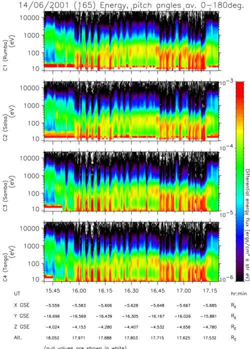
Fig. 1. Energy-time spectrograms of the electron populations observed by the 4 Cluster spacecraft between 15:40 UT and 17:20 UT on 14 June 2001. The data shown in each panel represents a direction-averaged composite of the differential energy fluxes recorded by the two PEACE sensors on each spacecraft, such that the full energy range is 10 eV to 32 keV. The colour bar for the flux levels is shown on the right, while the ephemera data for the reference spacecraft (Cluster 3) is shown at the bottom of the figure. During the period shown, the quartet was located on the dawn flank of the magnetosphere. The data indicate that all 4 spacecraft underwent a series of transitions between the magnetosheath (which exhibits intense differential energy fluxes peaked at energies of a few 10 s of eV) and the magnetosphere or magnetopause boundary layer (where the differential energy fluxes are less intense but peaked at energies of 100–200 eV). Note that the transitions between these two populations are rather periodic over this period, suggesting that the Cluster quartet is observing the effects of a magnetopause boundary wave during this period.
of each spacecraft between the magnetosphere and the mag-netosheath to calculate the speed and direction of those parts of the surface wave which cross the Cluster quartet. In the next section, we briefly discuss the instrumentation on board each of the Cluster spacecraft which is utilized in this study. In Sect. 3, we describe the Cluster observations made
CLUSTER C1234 FGM/C13 CIS 14 June 2001 -50 0 50 θB (degs) -100 0 100 φB (degs) 0 5 10 15 20 25 30 |B| (nT) 0.1 1.0 10.0 NI (cm -3) 10 100 1000 10000 TI (eV) -400 -200 0 200 400 VIX (km s -1) -400 -200 0 200 400 VIY (km s -1) 15:40:00 -5.6 -16.8 -4.0 16:05:00 -5.6 -16.6 -4.2 16:30:00 -5.6 -16.3 -4.4 16:55:00 -5.7 -16.1 -4.6 17:20:00 -5.7 -15.9 -4.8 -400 -200 0 200 400 VIZ (km s -1) UT XGSE (RE) YGSE (RE) ZGSE (RE) dX (km) dY (km) dZ (km) 1245 1832 586 -192 1128 1751 0 0 0 1251 -211 1672 1241 1997 525 -148 1248 1721 0 0 0 1268 -119 1702 1240 2174 467 -100 1375 1689 0 0 0 1284 -22 1730
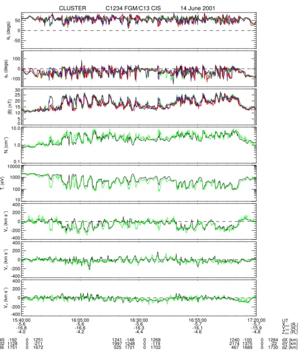
Fig. 2.Magnetic field and ion plasma data from the FGM and CIS instruments, respectively. Data from Cluster 1 is shown as the black traces, Cluster 2 in red, Cluster 3 in green and Cluster 4 in magenta. The top 3 panels contain the 4 spacecraft FGM data, showing the elevation angle,θB, the azimuth angle, φB, and strength|B|of the magnetic field vector. The lower 5 panels show the ion density, temperature,
and 3 components of the flow velocity observed by spacecraft 1 and 3. The cold dense plasma observed when the spacecraft are in the magnetosheath is associated with field strengths of|B|∼25 nT, while inside the magnetosphere the field strength of|B|∼15 nT. The field direction on the two sides of the boundary is similar and points strongly northward, with only small deflections in field direction at the transitions. Inside the magnetosphere the flow velocities are low,|V|<a few tens of km s−1, while in the magnetosheath an anti-sunward (−VX) flow of 100–200 km s−1is observed. The y-component of the flow shows an oscillation aboutVY=0.
2 Instrumentation
This study uses electron measurements from the PEACE (Plasma Electron And Current Experiment) instruments (Johnstone et al., 1997; Owen et al., 2001) on the 4 Cluster spacecraft, together with supporting observations of the mag-netic field by the FGM (Flux Gate Magnetometer) (Balogh
the energy of electrons measured by the low-energy electron analyzer (LEEA) covered the range∼1 eV to 1 keV, while the high-energy electron analyzer (HEEA) covered the range
∼40 eV to 26 keV. The FGM instrument consists of two tri-axial sensors capable of sampling up to 67 vectors/s. In this study we use spin resolution (4 s) magnetic field data. The CIS instrument provides information on the ion populations from thermal energies to about 40 keV/e.
3 Observations
On 14 June 2001 (day 165) the 4 Cluster spacecraft made multiple encounters with the dawnside flank magnetopause between∼16:00 and∼17:00 UT. At 16:30 UT the Cluster centroid was located at position (−5.5, −16.3, −4.2) RE (Earth radii) in the Geocentric Solar Ecliptic (GSE) coordi-nate system. Spectrograms summarizing the PEACE data taken during this period are shown in Fig. 1. The 4 panels in this figure show an energy-time spectrogram of the PEACE data recorded by each of the 4 spacecraft between 15:40 UT and 17:20 UT on this day. Each panel indicates the differ-ential energy flux observed between 10 eV and 26 keV, and thus is a composite of data obtained by both of the PEACE sensors on each spacecraft. These summary data consist of a direction-averaged electron flux derived on the ground from a 2-D sample of the full 3-D distribution that is returned from the spacecraft. This 2-D cut is taken from the plane that con-tains both the spacecraft spin vector and the instantaneous magnetic field direction. An appropriate transformation of this sample thus provides a measure of the pitch-angle dis-tribution of the ambient electron population, under the as-sumption that this is gyrotropic. Ephemera data for the ref-erence spacecraft (Cluster 3) are given at the bottom of the plot. Crossings of the magnetopause by each of the 4 space-craft can be identified in this figure by both the changes in the energy of the peak flux and the flux levels of the observed electrons as the spacecraft moves between the magnetosheath and magnetosphere. Specifically, observations of differen-tial energy fluxes of the order of 10−3ergs (cm2s str eV)−1 peaked between 10 and 100 eV, indicating that the spacecraft were sampling magnetosheath plasma, while maxima in the fluxes located between 100 and 300 eV represent observa-tions of boundary layer plasma inside the magnetosphere. The high fluxes of electrons at energies of∼10 eV and below are most likely a result of photo-electrons of spacecraft origin entering the instrument apertures and should be ignored.
The magnetic field data from the FGM instrument on each of the 4 spacecraft and ion plasma data from the CIS instru-ments on spacecraft 1 and 3 are shown in Fig. 2. (Black traces represent C1 data, red for C2, green for C3 and magenta for C4.) The top 3 panels show the GSE elevation angle,
θB, the azimuth angle,φB, of the magnetic field direction, and the magnitude of the magnetic field. In this represen-tation,θB=90◦represents a magnetic field pointing directly northward,θB=0◦ represents a magnetic field lying within the ecliptic plane, whileφB=0◦indicates a field with a
sun-ward component,φB=90◦a field with a duskward compo-nent. These 3 panels show that for the most part, the 4 space-craft observe similar magnetic fluctuations throughout this period. The transitions from the magnetosheath into the mag-netosphere (and vice versa) are marked by a change in the magnetic field strength, with the magnetosheath side having an average|B|∼25 nT, while that in the magnetosphere has a somewhat lower average value, |B|∼15 nT. However, the field direction is less variable between the two regions, and remains predominantly northward and dawnward (θB∼60◦,
φB=−50◦on average) on both sides. Short duration shifts in the direction of the magnetic field tend to occur at the bound-ary between the two plasma regions.
The lower 5 panels of Fig. 2 show the density, tempera-ture, and 3 components of the velocity of the ions detected by the CIS instruments on Clusters 1 and 3. In these pan-els, the transition across the boundary is marked by a change from a cold, dense plasma in the magnetosheath to a hotter, more rarified plasma inside the magnetosphere. In the latter region the plasma flow speeds are very low (V <a few tens of km s−1), while in the magnetosheath anti-sunward flows at speeds of 100–200 km s−1are observed. Note, also, that the y-component of the flow shows an oscillation aboutVY=0.
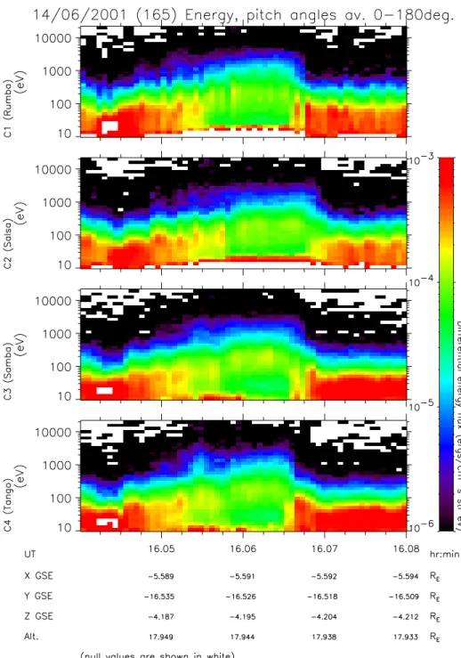
A more detailed set of PEACE spectrograms, for the 4-min period 16:04–16:08 UT, is shown in Fig. 3, in the same format as Fig. 1. These cover a transition of the 4 space-craft from the magnetosheath and into the magnetosphere at
boundary observed in the period described above are largely parallel. For this reason, the minimum variance analysis does not return a meaningful result for many of the boundary crossings observed during this period. The observed bound-aries are predominantly plasma boundbound-aries, and thus, in this study, we assess the boundary timings using the PEACE ob-servations.
Once the timings of the boundary crossings at each space-craft have been determined, this information can be used to deduce the motion of any given boundary, as described, for example, in Owen et al. (2001). In this method we must as-sume that the boundary is close to planar on the scale size of the spacecraft separation, and moves with constant velocity. The differences in the boundary observation times at each spacecraft position can then be used to calculate the speed and direction of motion normal to the boundary surface. As noted above, the nature of the magnetopause boundary cross-ings in the PEACE data is somewhat variable. However, to quantify the timings, the boundary crossings by each space-craft must be consistently identified within the data set. To do this, we use the bulk moments of the electron popula-tion calculated on board each spacecraft. In particular, we identify the local maxima in the time rate of change of elec-tron moments during the large changes that occur in these data at each boundary. Comparison of the results of this approach applied to both the density and scalar temperature moments revealed that the magnetopause crossings could be most readily identified from the gradients in the tempera-ture moments from each spacecraft. It should be noted that the technique employed here to determine boundary-crossing times is adopted principally as a method whereby some as-pect of the transition from the magnetosphere to the mag-netosheath can be consistently identified within the PEACE data set. Since the transition from the magnetosphere to the magnetosheath must involve crossing the magnetopause, we arbitrarily chose to associate this temperature gradient max-imum coincident with a large total change in temperature with the instant that each spacecraft makes a crossing of the magnetopause. We assume that any errors in the tim-ing between this temperature gradient maximum and the real magnetopause crossing are systematic and identical at each spacecraft, such that the timing analysis results are unaf-fected.
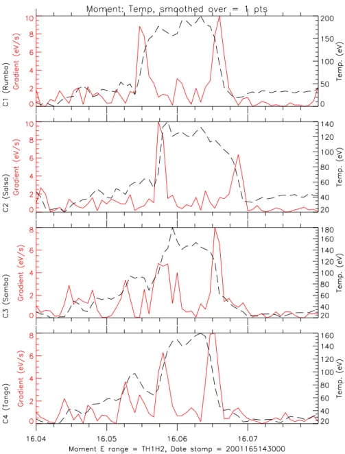
Figure 4 shows the temperature moment changes during the two magnetopause crossings previously shown in Fig. 3 above. The dashed line in this figure represents the effec-tive temperature of the electrons determined by taking a mo-ment summation of electron populations within the HEEA (40 eV to 26 keV) range, while the solid line indicates the magnitude of the gradient in this quantity. Note that for the most part, the large temperature changes are associated with a clear peak in the gradient. In the C3 data at 16:05:45 UT there is a less clear association, and in this case the earlier peak in the gradient is chosen as it coincided with a larger to-tal change in temperature than the later peak. Using the times identified as the peak gradient on each spacecraft, we can de-termine the motion of the boundaries as outlined above. For
the case shown in Fig. 3, we find that during the transition from the magnetosheath into the magnetosphere observed at
∼16:05:30 UT the timings are consistent with a boundary motion in the direction (−0.53, −0.58, 0.62) in GSE co-ordinates and at a speed of 118 km s−1 (i.e. GSE velocity components (−62, −68, 73) km s−1). Conversely, during the return transition from magnetosphere to magnetosheath at∼16:06:40 UT, the timings are consistent with a boundary motion in the GSE direction (−0.69, 0.46, 0.56) at a speed of 82 km s−1. The corresponding GSE velocity components are (−57, 38, 46) km s−1. Note that the boundary normals deter-mined here from the Cluster data can be directly compared to the normal calculated on the basis of the Fairfield (1971) model magnetopause scaled to the spacecraft position. This is calculated to be (0.32, −0.92, −0.23) in this coordinate system. Note, also, that although a minimum variance analy-sis of FGM data does not return a meaningful determination of the boundary normal at each spacecraft for many of the observed crossings, it can be used as a successful check on the 4-spacecraft timing result for those crossings that it is successful. For the first crossing evident in Fig. 3, the min-imum variance analysis of the corresponding magnetic field (not shown) fails. However, during the second crossing there are sufficient variances in the magnetic field to determine an MVA normal at the 4 spacecraft. In each case, the MVA normal is within 15◦of that determined by the 4-spacecraft method, thus validating the results of the latter method.
A total of 21 magnetosheath exits and 23 entries similar to those described above could be identified in the PEACE data during the period 15:55–17:15 UT and these were ana-lyzed using the above technique. The results of the boundary motion calculations for these crossings are summarized in Fig. 5, which is comprised of three panels showing, from top to bottom, the boundary velocities in theX−Y,X−Z and
Fig. 3. Energy-time spectrograms of the electron populations observed by the 4 Cluster spacecraft between 16:04 UT and 16:08 UT on 14 June 2001. The figure is in the same format as Fig. 1, but covers a shorter time period, during which the Cluster quartet made a single transition from the magnetosheath into the boundary layer (∼16:05:15 UT) and then back into the magnetosheath (∼16:06:30 UT). Note that the entries by all 4 spacecraft into the magnetosphere at∼16:05:15 UT appear to be a more gradual transition than the exits at∼16:06:30 UT, which show a much more discontinuous change in the electron fluxes. This single entry-exit transition has characteristics that are largely representative of all the other transitions evident in Fig. 1.
northern component than the entries. The average over all the velocity magnitudes is∼100 km s−1, with the average mag-nitude of the exit velocities being∼120 km s−1and the en-try velocities∼80 km s−1. The angles between the boundary motion normals determined from the inter-spacecraft timings and the model MP normal ((0.32,−0.92,−0.23) in GSE
Fig. 4. Electron scalar temperature variations (dashed line, right-hand scale) observed by the 4 Cluster spacecraft between 16:04 UT and 16:08 UT on 14 June 2001 (c.f. Fig. 3). The transitions between the cool (∼30–40 eV) magnetosheath and warmer boundary layer (>100 eV) plasmas are evident in each panel. The solid lines (related to the left-hand scale) indicate the magnitude of the gradient in these temperature profiles between each measurement. Relatively clear peaks occur in this parameter for each major transition in plasma temperature. These peaks are used as a measure of the time that the boundary between the two plasma populations crosses each of the 4 spacecraft, and thus to determine the orientation and speed of this boundary (see text).
these angles would be 0◦for entries into the magnetosphere, associated with dawnward motion of the boundary, and 180◦ as the boundary moves duskward to return the spacecraft to the magnetosheath. The dashed lines in each panel represent the average normal angle for all the magnetospheric exit and entry events, respectively. Note that the angles associated with entries to the magnetosphere are more variable than the angles during exit. The mean normal angle during entries is 68◦away from the model magnetopause normal, i.e. only 22◦out of the plane of the model magnetopause itself and pointing into the magnetosheath (i.e. somewhat dawnward).
In contrast, the mean angle during exits is 138◦, or 42◦away from the model magnetopause plane and pointing into the magnetosphere.
4 Discussion
BOUNDARY MOTIONS 16:00-17:00 UT 14 June 2001
-6.4 -6.1 -5.8 -5.5 -5.2
XGSE (RE)
-17.0 -16.7 -16.4 -16.1 -15.8
YGSE
(R
E
)
100 km s
-1
-6.4 -6.1 -5.8 -5.5 -5.2
XGSE (RE)
-5.0 -4.7 -4.4 -4.1 -3.8
ZGSE
(R
E
)
100 km s
-1
-17.0 -16.7 -16.4 -16.1 -15.8
YGSE (RE)
-5.0 -4.7 -4.4 -4.1 -3.8
ZGSE
(R
E
)
100 km s
-1
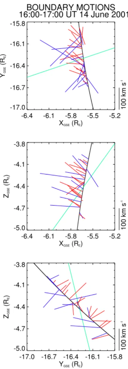
Fig. 5. Results of the boundary motion analysis for each of the transitions evident in Fig. 1. The 3 panels show the motion of the boundary projected onto each of theX−Y, X−Z andY−Z
GSE planes. The intersection of the Fairfield (1971) model mag-netopause surface (scaled to the spacecraft location at 16:30 UT) with each plane is shown as the green curve in each panel. The spacecraft trajectory projected onto each plane is shown as the black trace. The projection of vectors representing the speed and normal direction of motion of each magnetosheath-magnetosphere bound-ary in each plane are shown extending from the point on the orbit trajectory corresponding to their time of observation. Vectors de-termined for transitions from magnetosheath to magnetosphere are shown in red, while those for transitions in the opposite sense are shown in blue. The length of a vector representing 100 km s−1is indicated at the bottom of the plot. From these results it is clear that most boundary motions involve motion in the negativeXGSE
direc-tion, indicating a tailward propagation of the wavetrain. In theY−Z
plane (lower panel) it is also clear that most boundaries move in the general directions expected for inbound/outbound crossings of the magnetopause, consistent with motions of the magnetopause driven by a set of boundary waves moving across the spacecraft locations.
large-scale breathing motion of the magnetopause. Indeed, since the Cluster quartet is located close to the equatorial flank of the magnetosphere, any large-scale inward/outward breathing of the magnetopause should manifest itself as a predominant positive/negativey-component of the boundary velocity. This oscillation is also seen in theVY component of the ion velocity presented in Fig. 2. Clearly, however, both the inbound and outbound boundary motions, consistent with the data shown in Fig. 4, have significant negative x- and positivez-components to their motion, indicating a bound-ary wave structure with wave fronts moving along the mag-netopause in these directions. An anti-sunward (i.e. negative x-directed) component of motion is perhaps not surprising for boundary waves that may be driven by the magnetosheath flow. However, the strong, positivez-component to the mo-tion is perhaps unexpected, especially as the Cluster quartet is located slightly below the ecliptic plane where models of the exterior magnetosheath flow (e.g. Spreiter and Stahara, 1980) indicate a small component of flow in the negativez -direction. Indeed, no significantz-component of the flow ve-locity is observed by the CIS instrument (Fig. 2) during the period under consideration.
BOUNDARY CHARACTERISTICS 1545-1715 UT 14 June 2001
0 45 90 135 180
Exit angle (deg.)
0 45 90 135 180
Entry angle (deg.)
0.0 0.5 1.0 1.5 2.0 2.5
C1 Stability
15.45 16.00 16.15 16.30 16.45 17.00 17.15
Time (UT) 0.0
0.5 1.0 1.5 2.0 2.5
C3 Stability
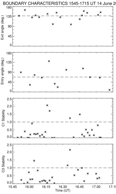
Fig. 6.Upper 2 panels: Plots of the angles between the boundary normals determined from the 4-spacecraft measurements and the Fairfield (1971) model magnetopause normal as a function of time of observation of each boundary. The upper panel shows the angles determined during transitions from the magnetosphere into the magnetosheath, while the lower panel shows those angles determined during transitions in the opposite sense. The dashed line in each panel represents the mean angle for the appropriate data set. Note that the wavefronts during the latter transition are, on average, 79◦away from the direction expected on the basis of the model magnetopause. In contrast, the transitions from magnetosphere into the magnetosheath are only 34◦away from the expected direction (along the inward pointing model normal). Thus, the wavefronts associated with the former transition appear to be significantly steeper inclined, on average, compared to the latter. Lower Panels: Results of a Kelvin-Helmholtz stability analysis (c.f. Eq. (1)) for the magnetopause boundary based on data from Clusters 1 and 3. The vertical axes of these panels show the ratioRof the two terms on either side of the inequality symbol in Eq. (1), such that values of
R>1 (i.e. above the dashed line in each panel) indicate the magnetopause to be Kelvin-Helmholtz unstable. For most of the period under discussion, it appears that the magnetopause is stable to this mechanism. However, the brief periods for which instability is indicated appear to correspond to times in which the angles of the observed wavefronts (upper 2 panels) are furthest from the expectations for an undisturbed model magnetopause. This indicates that the wavefronts are steepest during these times.
analysis as the spacecraft exits the magnetosheath are steeper than the entry angles is most likely appropriate. In addition, we note that our results are consistent with those of some other studies (e.g. Fairfield et al., 2000).
plasma velocities V1 and V2 on either side of a boundary
crossing which are provided by the CIS instruments, the magnetic fieldsB1andB2provided by the FGM instrument
and the electron number density n from PEACE. In order to make an assessment of k, the unit wave vector, we
ro-tate the mean observed boundary normal,nBDY, (for pairs of
magnetosphere entries and exits) into the plane of the model magnetopause viak=nMP×(nBDY×nMP), where nMP is
the model magnetopause normal. The results of the instabil-ity analysis for C1 and C3 are shown in the lower panels of Fig. 6. The CIS ion data from C2 and C4 were not avail-able during this interval and thus, we are unavail-able to perform this analysis on the observations from these spacecraft. In the lower panel, we show the ratio, R, of the terms on each side of the inequality sign in Eq. (1), such that a value of R larger than unity suggests an unstable boundary. For most of the interval, the analysis indicates that the waves are Kelvin-Helmholtz stable (R<1). However, when comparing these results to the wave exit and entry angles in the upper panels, we find that instances where the observed data are consis-tent with the magnetopause being Kelvin-Helmholtz unsta-ble (R>1) generally occur in association with increases in the wave exit angle, i.e. a steepening of the leading edge of the wave. The Kelvin-Helmholtz instability is predicted to cause such a steepening of the leading edge of surface waves (Miura, 1990), consistent with our observations. However, waves generated by means other than the Kelvin-Helmholtz mechanism might also be expected to show a similar trend between their leading and trailing edges, such that this alone does not provide a conclusive identification of the wave driv-ing mechanism. Although the above analysis is inconclusive in this case, it is informative to consider the general orienta-tion of the boundary wave fronts to the magnetosheath field and flow directions. As mentioned above, the wave fronts generally appear to have a positivez-component to their mo-tion, despite the location some 4.5RE south of the ecliptic plane. During this period, the average magnetic field ob-served while the spacecraft are in the magnetosheath is (11.5,
−3.4, 17.7) nT, while in the magnetosphere the average field (6.4,−3.9, 14.2) nT. The average fields on either side of the magnetopause boundary are thus close to parallel, separated in direction by only about 10◦. Moreover, the fields point predominantly in the positiveX- and positiveZ-directions, which is approximately perpendicular to the direction of mo-tion of the wave fronts inferred above. For this direcmo-tion of motion, therefore, the magnetic fields on either side of the boundary lies along the crests and troughs of the wave, as also indicated in the sketch in Fig. 7. Hence, the wave ap-pears to be moving in the one direction in which the mag-netic fields on either side of the magnetopause do not need to be sharply bent in order to accommodate the wave, and that most energy is, therefore, available for the wave growth. This can also be seen mathematically in Eq. (1), in which the termsk.Bare smallest, and thus the inequality most likely to
be satisfied, if the wave vectorkis perpendicular to the
mag-netic fieldB. This appears to be the case, at least on average,
in the event presented here.
n
MP
n
IN
n
OUT
Magnetosphere
Sheath
Wave motion
(in –ve X- and +ve Z-direction)
3.4 R
E~ 65 km s
-1B
SH
B
SPH
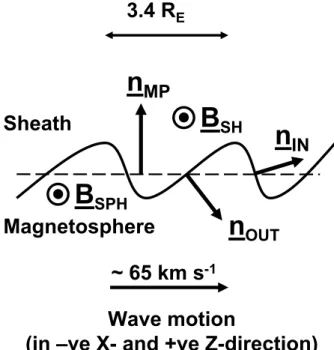
Fig. 7.Sketch illustrating the average structure of the magnetopause surface wave consistent with the results of the 4-spacecraft timing analysis. These results suggest that the leading edge of the waves, associated with transitions of the spacecraft from magnetosheath to magnetosphere, are inclined from the expected orientation of the undisturbed magnetopause by a larger angle, on average, than the trailing edge associated with transitions in the opposite sense. In addition, the direction of propagation of the waves, in the negative GSEX- and positiveZ-directions, is close to perpendicular to the magnetic fields on either side of the boundary. This suggests that the wave growth and propagation occurs preferentially in the direction in which the wave does not have to bend the surrounding lines of magnetic force.
Finally, the wavelength of these surface waves can be estimated by using the mean velocity of the waves across the magnetopause (∼65 km s−1) and the time differences be-tween pairs of boundary crossings. In this manner, we find the mean wavelength is approximately 3.4RE.
5 Conclusions
4 spacecraft have been used to determine the local orienta-tion and speed of the associated magnetopause boundary as it moves back and forth over the spacecraft location. These orientations can be compared with the expectations for the average magnetopause orientation determined from model fits to historical data (e.g. Fairfield, 1971). This compar-ison reveals that both the inbound and outbound crossings of the magnetopause are significantly deflected from the ex-pected orientation, in the senses that are indeed consistent with the passage of a boundary wave past the spacecraft loca-tion. We find also that the leading edge of the wave is signifi-cantly steeper in inclination to the model magnetopause than the trailing edge. This observation is consistent with expec-tations of Kelvin-Helmholtz waves (and possibly waves of other origin), but contradicts the conclusions of the 2 space-craft study presented by Chen et al. (1993). We tested the conditions on either side of the magnetopause to determine whether they satisfied the conditions for this boundary to be Kelvin-Helmholtz unstable, based on the simple incompress-ible plasma model. The boundary was found to be largely stable during this period. However, we note that there is some suggestion in the results that the sub-intervals which satisfy the instability criterion are closely matched in time with the steepest boundary orientations. The 4-spacecraft timing results can also be used to determine the wavelength of the surface waves and their speed and direction of prop-agation across the model magnetopause surface. For this event, we find an average wavelength of∼3.4RE, and that the waves propagate at an average speed of∼65 km s−1in an anti-sunward and northward direction. The northward com-ponent to the motion is unexpected, since the spacecraft are located south of the GSEZ=0 plane, where the large-scale magnetosheath flow outside the magnetopause is expected to have a southward component at this location. Indeed, the ion flows observed when the spacecraft are in the magnetosheath (c.f. Fig. 2) do not show a significant northward compo-nent. However, the propagation direction is approximately perpendicular to the average external magnetic field direc-tion, suggesting that these waves may preferentially propa-gate in the direction which requires no bending of magnetic lines of force. Although this observation is also consistent with waves driven by the KHI, which are expected to grow fastest whenk.B is small, it may also be the energetically
most favourable conditions for the growth of other waves. Hence, although the waves show characteristics that might be expected of those driven by the KHI, we are unable at present to definitively identify them as such.
Acknowledgements. This work was funded by the UK Particle
Physics and Astronomy Research Council (PPARC). In particu-lar, CJO would like to acknowledge support via a PPARC Ad-vanced Fellowship. We also thank Cluster Principal Investigators A. Balogh and H. R`eme for use of FGM and CIS data in this study. Topical Editor T. Pulkkinen thanks D. Fairfield and another ref-eree for their help in evaluating this paper.
References
Axford, W. I. and Hines, C. O. : A unifying theory of high-latitude geophysical phenomena and geomagnetic storms, Can. J. Phys., 39, 1433–1464, 1961.
Balogh, A., Carr, C. M., Acuna, M. H., Dunlop, M. W., Beek, T. J., Brown, P., Fornacon, K.-H., Georgescu, E., Glassmeier, K.-H., Harris, J., Musmann, G., Oddy, T., and Schwingenschuh, K.: The Cluster magnetic field investigation: overview of in-flight per-formance and initial results, Ann. Geophysicae, 19, 1207–1217, 2001.
Chandresekhar, S.: Hydrodynamic and Hydromagnetic Stability, Clarendon, Oxford, 1961.
Chen, S.-H. and Kivelson, M. G.: On Non-Sinusoidal Waves at the Earths Magnetopause, Geophys. Res. Lett., 20, 2699–2702, 1993.
Chen S.-H., Kivelson, M. G., Gosling, J. T., Walker, R. J., and Lazarus, A. J.: Anomalous Aspects of Magnetosheath Flow and of the Shape and Oscillations of the Magnetopause During an Interval af Strongly Northward Interplanetary Magnetic Field, J. Geophys. Res., 98, 5727–5742, 1993.
Drazin, P. G. and Reid, W. H.: Hydromagnetic Stability, Cambridge University Press, 1985.
Dungey, J. W.: Electrodynamics of the outer atmosphere, in Pro-ceedings of the ionosphere Conference, The Physical society of London, 225, 1955.
Dungey, J. W.: Interplanetary magnetic field and the auroral zones, Phys. Rev. Lett., 6, 47–48, 1961.
Dunlop, M. W. and Woodward, T. I.: Discontinuity analysis: ori-entation and motion, in: Analysis methods for multispacecraft data, ISSI Scientific Report SR-001, ESA Publications, Noord-wijk, The Netherlands, 271, 1998.
Fairfield, D. H.: Average and unusual locations of the Earths mag-netopause and bow shock, J. Geophys. Res., 76, 6700–6716, 1971.
Fairfield, D. H., Otto, A., Mukai, T., Kokubun, S., Lepping, R. P., Steinberg, J. T., Lazarus,A. J., and Yamamoto, T.: GEOTAIL observations of the Kelvin-Helmholtz instability at the equatorial magnetotail boundary for parallel northward fields, J. Geophys. Res., 105, 21 159–21 174, 2000.
Farrugia, C. J., Gratton, F. T., Bender, L., Biernat, H. K., Erkaev, N. V., Quinn, J. M., Torbert, R. B., and Dennisenko, V.: Charts of joint Kelvin-Helmholtz and Rayleigh-Taylor instabilities at the dayside magnetopause for strongly northward interplanetary magnetic field, J. Geophys. Res., 103, 6703–6727, 1998. Farrugia, C. T., Gratton, F. T., Contin, J., Cocheci, C. C., Arnoldy,
R. L., Ogilvie, K. W., Lepping, R. P., Zastenker, G. N., Noz-drachev, M. N., Federov, A., Sauvaud, J.-A., Steinberg, J. T., and Rostoker, G.: Coordinated Wind, Interball/tail, and ground ob-servations of Kelvin-Helmholtz waves at the near-tail, equatorial magnetopause at dusk: 11 January 1997, J. Geophys. Res., 105, 7639–7667, 2000.
Fitzenreiter, R. J. and Ogilvie, K. W.: Kelvin-Helmholtz Instability at the Magnetopause: Observations, in Physics of the Magne-topause, edited by Song, P., Sonnerup, B. U. ¨O., and Thomsen, M. F., AGU monograph, 277–284, 1995.
Kivelson, G. K. and Chen, S.-H.: The Magnetopause: Surface waves and Instabilities and their possible Dynamical Conse-quences, in Physics of the Magnetopause, edited by: Song, P., Sonnerup, B. U. ¨O, and Thomsen, M. F., AGU monograph, 257– 268, 1995.
Miura, A.: Anomalous transport by magnetohydrodynamic Kelvin-Helmholtz instabilities in the solar wind-magnetosphere interac-tion, J. Geophys. Res., 89, 801–818, 1984.
Miura, A.: Kelvin Helmholtz instability for supersonic shear flow at the magnetopause boundary, Geophys. Res. Lett., 17, 749–752, 1990.
Miura, A.: Kelvin-Helmholtz Instability at the Magnetopause: Computer Simulations, in Physics of the Magnetopause, edited by Song, P., Sonnerup, B. U. ¨O, and Thomsen, M. F., AGU monograph, 285–291, 1995.
Nykyri, K. and Otto, A.: Plasma transport at the magnetospheric boundary due to reconnection in Kelvin-Helmholtz vortices, Geophys. Res. Lett., 28, 3565–3568, 2001.
Ogilvie, K. W. and Fitzenreiter, R. J.: The Kelvin-Helmholtz insta-bility at the magnetopause and the inner boundary layer surface, J. Geophys. Res., 94, 15 113–15 123, 1989.
Otto, A. and Fairfield, D. H.: Kelvin-Helmholtz instability at the magnetotail boundary: MHD simulation and comparison with GEOTAIL observations, J. Geophys. Res., 105, 21 175–21 190, 2000.
Owen, C. J., Fazakerley, A. N., Carter, P. J., Coates, A. J., Krauk-lis, I. C., Szita, S., Taylor, M. G. G. T., Travnicek, P., Watson, G., Wilson, R. J., Balogh, A., and Dunlop, M. W.: CLUSTER PEACE Observations of Electrons During Magnetospheric Flux Transfer Events, Ann. Geophysicae, 19, 1509–1522, 2001. Pu, Z.-P. and Kivelson, M. G.: Kelvin-Helmholtz instability at the
magnetopause: Solution for compressible plasma, J. Geophys. Res., 88, 841–852, 1983a.
Pu, Z.-P. and Kivelson, M. G.: Kelvin-Helmholtz instability at the magnetopause: Energy flux into the magnetosphere, J. Geophys. Res., 88, 853–861, 1983b.
R`eme, H., Aoustin, C., Bosqued, J. M., et al.: First multispacecraft ion measurements in and near the Earth’s magnetosphere with the identical Cluster ion spectrometry (CIS) experiment, Ann. Geophysicae, 19, 1303–1354, 2001.
Russell, C. T. and Elphic, C.: ISEE observations of flux transfer events at the dayside magnetopause, Geophys. Res. Lett., 6, 33– 36, 1979.
Seon, J., Frank, L. A., Lazarus, A. J., and Lepping, R. P.: Sur-face waves on the tailward flanks of the Earth’s magnetopause, J. Geophys. Res., 100, A7, 11 907–11 922, 1995.
Sibeck, D. G., Paschmann, G., Treumann, R. A., Fuselier, S. A., Lennartsson, W., Lockwood, M., Lundin, R., Ogilvie, K. W., Onsager, T. G., Phan, T.-D., Roth, M., Scholer, M., Sckopke, N., Stasiewicz, K., and Yamauchi, M.: Plasma transfer processes at the magnetopause, Space Sci. Rev., 88, 207–283, 1999. Southwood, D. J.: The hydromagnetic stability of the
magneto-spheric boundary, Planet. Space Sci., 16, 587–605, 1968. Southwood, D. J. and Hughes, W. J.: Theory of hydromagnetic
waves in the magnetosphere, Space Sci. Rev., 35, 301–366, 1983. Spreiter, J. R. and Stahara, S. S.: A new predictive model for de-termining solar wind-terrestrial planet interactions, J. Geophys. Res., 85, 6769–6777, 1980.
Treumann, R. A., Labelle, J., and Bauer, T. M.: Diffusion Processes: An Observation Perspective, in: Physics of the Magnetopause, edited by Song, P., Sonnerup, B. U., ¨O., and Thomsen, M. F., AGU monograph, 331–341, 1995.