The comparison of measured impedance of the bladder tissue with the computational modeling results

* Corresponding Author: Ahmad Keshtkar, Email: mpp98ak@hotmail.com

© 2015 The Authors; Tabriz University of Medical Sciences

The comparison of measured impedance of the bladder tissue with the

computational modeling results

1 _{Professor, Department of Medical Physics, School of Medicine, Tabriz University of Medical Sciences, Tabriz, Iran}

2 _{Professor, Department of Urology, School of Medicine, Imam Reza Teaching Hospital, Tabriz University of Medical Sciences, Tabriz, Iran}

Citation: Keshtkar A, Madaen SK. The comparison of measured impedance of the bladder tissue with the computational modeling results. J Anal Res Clin Med 2015; 3(4): 225-30. Doi: 10.15171/jarcm.2015.035

The finite element method has previously been applied to cervical and esophagus tissues.1,2 _{Before the normal esophagus}

changes to the cancerous esophagus, the tissue undergoes metaplasia from normal stratified squamous to a columnar epithelium. Differences in the electrical impedance spectra of the tissues appear to be explained by changes in cell arrangements and in the extra-cellular space. This suggests that an indication of tissue structure may be able to be derived from electrical impedance spectral measurements. Brown et al. measured the electrical impedance of cervix tissue.3 _{According to their work, the}

measured electrical impedance made on normal squamous tissues was well-separated from that made on pre-cancerous tissues.4

The impedance of normal areas was more than the impedance of abnormal areas.

It was hypothesized that the

characterization of the electrical impedance spectrum of cervical tissue is related to cellular arrangements of the tissue. After that Walker et al.4,5 _{modeled the electrical impedivity of}

normal, and premalignant cervical tissue using finite element analysis (FEA) to find the related electrical impedance.

Gonzalez-Correa et al.6 _{measured the}

electrical impedance of the esophagus tissue. They showed that the squamous and The electrical impedance spectroscopy technique can be used to measure the electrical impedance of the human bladder tissue, for differentiating pathological changes in the urothelium.

In this study, the electrical impedance spectroscopy technique and then, a numerical technique, finite element analysis (FEA) were used to model the electrical properties of this tissue to predict the impedance spectrum of the normal and malignant areas of this organ.

After determining and comparing the modeled data with the experimental results, it is believed that there are some factors that may affect the measurement results. Thus, the effect of inflammation, edema, changes in the applied pressure over the probe and the distensible property of the bladder tissue were considered. Furthermore, the current distribution inside the human bladder tissue was modeled in normal and malignant cases using the FEA. This model results showed that very little of the current actually flows through the urothelium and much of the injected current flows through the connective tissue beneath the urothelium.

The results of the models do not explain the measurements results. In conclusion, there are many factors, which may account for discrepancies between the measured and modeled data. Bladder,

Computational Modeling,

Electrical Impedance Measurement, Normal, Malignant

columnar tissues of the esophagus could be

separated by electrical impedance

spectroscopy. Furthermore, in this case, the impedance of normal areas was more than the impedance of malignant areas. They expected that it is possible to separate these tissue types using a data modeling process. Then, Jones1 _{used finite element modeling to}

model the electrical properties of normal and pre-cancerous esophageal tissue.

This modeling method was used to model the electrical properties of squamous and glandular columnar epithelia of the gastrointestinal tract to characterize the electrical properties of these tissues. The output from this model was compared with the measured impedance spectra. According to this comparison, the modeling confirmed the difference between the impedance of columnar and squamous tissues, but the modeled impedance varied significantly depending on the amount of surface fluid present.1 _{Keshtkar et al.}7 _{measured the}

electrical impedance of the urinary bladder tissue, and they found that the impedance of malignant area was significantly more than the impedance of the normal area.

Moreover, the finite element method was used to model the benign and malignant bladder tissue. Results of both measured impedance and modeling methods are in opposite each other. The impedance resulting from this model, for the malignant area was significantly less than the impedance of the normal area. We will realize this problem here.

Electrical impedance measurement method

The electrical impedance of the human urinary bladder is measured at different frequencies according to the spectroscopy systems (the applied current to measure the impedance is very low). This constant current passed through two electrodes of a small sized probe that was designed and constructed by author.8 _{These electrodes constructed of four}

gold wire electrodes, 0.5 mm in diameter, spaced equally on a 1.6 mm diameter circle.

Total diameter of the probe was only

2 mm thus it was limited because of the maximum permitted diameter of the endoscopic channel to pass the probe towards the inside of the urinary bladder during the bladder surgery.

Detailed information about this probe can be found in Keshtkar and Smallwood9 _and

Smallwood et al.10 _{As we know, the most}

common form of measuring tissue

impedance is the tetra-polar or the 4-electrode technique. In this technique, a known current is driven between two electrodes, and the resulting voltage is measured between the other two electrodes.

Therefore, the resulting potential was measured using this technique to obtain the impedance of the urothelium. In impedance data collection procedure, the probe regularly was calibrated using known conductivity of saline solutions before any measurement procedure to have the tissue impedance readings in terms of the impedivity in Ωm.

The measured impedance data was recorded in a laptop in order for further data analysis. There is a study by author that explains how we can measure the electrical impedance data of the human bladder tissue in benign and malignant cases.7 _{In addition, there}

is a paper from the author to relate the effect of inflammation and edema on the resulting electrical impedance of the urinary bladder tissue in the form of increasing and decreasing of the related impedance, respectively.10

Finite element modeling method

For the purpose of modeling tissue structure, it is easier if cells are modeled as simple geometric shapes. Geometrical and physical parameters of the urothelium were used in this study to construct a high-resolution model of the cell. Geometric parameters, such as cell size were obtained from the observation of histology sections.8,11

layers) for malignant and benign groups was calculated. Keshtkar et al.11 _{for more details}

about this imaging technique to calculate the morphological parameters.

Electrical conductivities obtained from the cellular level models were assigned as material properties to epithelial layers in the macroscopic tissue model. This model consisted of three epithelial layers representing superficial, intermediate and basal cell types, underlying layers representing the basement membrane and connective tissue, and a surface layer of variable thickness, representing a thin layer of mucus or surface fluid.

Furthermore, the macroscopic tissue

model was constructed using the

experimental morphological parameters for bladder samples. There is no published data for the electrical properties of the basement membrane, so models were solved using the published conductivity and permittivity values for the tendon.12 _{The conductivity of}

the underlying connective tissue was based on conductivity values previously measured from unfixed healthy cervical stroma2 _and

permittivity published in the literature for the uterus.12 _{The mucus layer was assigned}

similar properties to those used for extra-cellular fluid.

Current was applied to the drive electrodes in the macroscopic model in the frequency range 100 Hz-10 MHz, and voltages calculated at the receiver electrodes in an identical arrangement to the in vivo tissue measurements. The impedance value obtained is equivalent to a calibration factor, by which all raw modeled impedances can be

divided to obtain impedivities in Ωm.

It is, therefore, possible to directly compare plots of impedivity against frequency obtained from the model with those obtained experimentally. Finally, the current flowing through every node located on the boundary midway between the two drive electrodes was calculated and then integrated to give the total current flowing through each layer. This information can provide an indication of the current distribution in vivo. Various model

parameters can be altered at either the cellular or the macroscopic stage of the modeling process in order to assess the effect on the impedance spectrum or the current distribution. Models were solved with mucus layer thicknesses in the range 5-100 m.

The real part of the complex impedance spectra of the human urinary bladder tissue was measured in different frequencies and is shown as figure 1. There are inflammation and edema effects on this measured impedance that the paper was published by author.10

According to this study, inflammation will increase the related measured electrical impedance and edema will decrease the electrical impedance. Therefore, these effects must be considered during the impedance measurements of the bladder tissue. Following this, the real part of the complex impedance spectra modeled using parameters obtained for relaxed benign and malignant cells parameters measured from histology sections are shown in figure 2A.

Figure 1. Real part of impedivity versus log of

frequency for normal and malignant bladder tissue7

Figure 2. The real part of the complex modeled impedance spectra for normal and malignant urothelium (A and B).

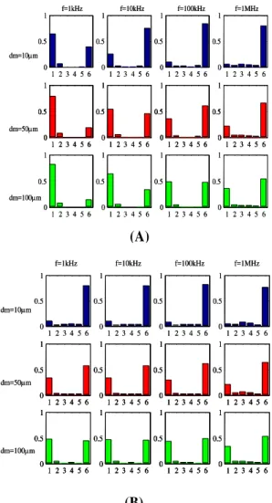
Figure 3 shows the proportion of the total current flowing through each of the macroscopic model layers-surface fluid and different parts of urothelium in both normal and malignant tissue models.

However, the model predicts that at frequencies less than 100 kHz, impedances measured from benign tissue should be higher than those measured from malignant tissue. This is the opposite situation to that suggested by the measured data, where higher impedances are measured from abnormal tissue (Figure 1). The model results also suggest that impedance spectra associated with normal tissue structure are sensitive to the thickness of the mucus or fluid layer at the tissue surface, whereas those associated with abnormal tissue are not. We can gain a greater understanding of this behavior by examining the current distribution in the normal and malignant models as following sentences. Figure 3 (A, B) shows the proportion of the total current flowing through each of the macroscopic model layers-surface fluid, superficial urothelium, intermediate urothelium, basal urothelium, basement membrane, and connective tissue respectively, in the normal tissue model. Data is shown for a number of frequencies and for three thicknesses of the surface fluid.

Figure 3. Modeled current-depth distribution midway

between drive electrodes for normal tissue model (A), malignant tissue model (B) at different frequencies and

surface layer thicknesses (dm)

Layer no. key: 1- surface fluid, 2- superficial urothelium, 3- intermediate urothelium, 4- basal urothelium, 5- basement

membrane, and 6- connective tissue

1 2 3 4 5 6 0 0.5 1

1 2 3 4 5 6 0 0.5 1

1 2 3 4 5 6 0 0.5 1

1 2 3 4 5 6 0 0.5 1

1 2 3 4 5 6 0 0.5 1

1 2 3 4 5 6 0 0.5 1

1 2 3 4 5 6 0 0.5 1

1 2 3 4 5 6 0 0.5 1

1 2 3 4 5 6 0 0.5 1

1 2 3 4 5 6 0 0.5 1

1 2 3 4 5 6 0 0.5 1

1 2 3 4 5 6 0 0.5 1

f=1kHz f=10kHz f=100kHz f=1MHz

dm=10m

dm=50m

dm=100m

1 2 3 4 5 6 0 0.5 1

1 2 3 4 5 6 0 0.5 1

1 2 3 4 5 6 0 0.5 1

1 2 3 4 5 6 0 0.5 1

1 2 3 4 5 6 0 0.5 1

1 2 3 4 5 6 0 0.5 1

1 2 3 4 5 6 0 0.5 1

1 2 3 4 5 6 0 0.5 1

1 2 3 4 5 6 0 0.5 1

1 2 3 4 5 6 0 0.5 1

1 2 3 4 5 6 0 0.5 1

1 2 3 4 5 6 0 0.5 1

1 2 3 4 5 6 0 0.5 1

1 2 3 4 5 6 0 0.5 1

1 2 3 4 5 6 0 0.5 1

1 2 3 4 5 6 0 0.5 1

f=1kHz f=10kHz f=100kHz f=1MHz

dm=10m

dm=50m

dm=100m

1 2 3 4 5 6 0 0.5 1

1 2 3 4 5 6 0 0.5 1

1 2 3 4 5 6 0 0.5 1

1 2 3 4 5 6 0 0.5 1

1 2 3 4 5 6 0 0.5 1

1 2 3 4 5 6 0 0.5 1

1 2 3 4 5 6 0 0.5 1

1 2 3 4 5 6 0 0.5 1

1 2 3 4 5 6 0 0.5 1

1 2 3 4 5 6 0 0.5 1

1 2 3 4 5 6 0 0.5 1

1 2 3 4 5 6 0 0.5 1

f=1kHz f=10kHz f=100kHz f=1MHz

dm=10m

dm=50m

dm=100m

1 2 3 4 5 6 0 0.5 1

1 2 3 4 5 6 0 0.5 1

1 2 3 4 5 6 0 0.5 1

1 2 3 4 5 6 0 0.5 1

1 2 3 4 5 6 0 0.5 1

1 2 3 4 5 6 0 0.5 1

1 2 3 4 5 6 0 0.5 1

1 2 3 4 5 6 0 0.5 1

1 2 3 4 5 6 0 0.5 1

1 2 3 4 5 6 0 0.5 1

1 2 3 4 5 6 0 0.5 1

1 2 3 4 5 6 0 0.5 1

1 2 3 4 5 6 0 0.5 1

1 2 3 4 5 6 0 0.5 1

1 2 3 4 5 6 0 0.5 1

1 2 3 4 5 6 0 0.5 1

1 2 3 4 5 6 0 0.5 1

1 2 3 4 5 6 0 0.5 1

1 2 3 4 5 6 0 0.5 1

1 2 3 4 5 6 0 0.5 1

f=1kHz f=10kHz f=100kHz f=1MHz

dm=10m

dm=50m

dm=100m

(A)

Figure 3B shows similar data for the malignant tissue model. It is immediately apparent that very little of the current actually flows through the urothelium itself (layer 2-4), but is divided between the surface fluid and underlying connective tissue at a ratio which depends on current frequency, depth of surface fluid and urothelial pathology. In the case of normal tissue, the presence of tight junctions and narrow intercellular spaces forms a very high impedance barrier, and at low frequencies in particular, current is confined to the surface fluid.

As the frequency is increased, the capacitive nature of cell membranes allows current flow into the surface cells, effectively

“short-circuiting” the tight junctions and

allowing current to penetrate beneath the epithelium and into the relatively high conductivity connective tissue beneath, thus causing the characteristic drop in tissue impedance with increasing frequency. However, our malignant superficial cell models do not include tight junctions, and the extra-cellular space is also wider, so the barrier to current flow is greatly reduced, even at low frequencies.

Figure 3B shows that at least 50% of the injected current flows beneath transformed urothelium across the frequency range modeled. The results of the models do not explain the measurements recorded in vivo and ex vivo, where higher impedances were measured from tissue independently diagnosed as malignant, but are in agreement with measurements and models of other squamous epithelia, where malignancy results in a reduction in electrical impedance, Gonzalez-Correa et al.6 _and

Bertemes-Filho et al.13

Surface plaques are not included in this model, and though these structures are extremely small, it is possible that they might influence the electrical properties of the tissue in a non-intuitive way. The model results, figure 3 shows that much of the injected current flows through the connective tissue beneath the urothelium.

Again, there is no data available for the electrical properties of this layer, so data

measured from the cervical stroma was used in this model, but may not be applicable to the bladder tissue, which contains a higher density of muscle that the cervical tissue. Furthermore, it is much more difficult to obtain good quality, histological sections of bladder epithelium, and in particular, there is little quantitative data available on the morphology of stretched bladder tissue. It is virtually impossible to find information on the distribution of extracellular space (ECS) in normal and carcinoma in situ (CIS) bladder, so it may be possible that the assumption that ECS increases with CIS, which was made when constructing the computational models, may be incorrect, and hence at least partially explain the different results. The modeling information presented here focused on changes within the urothelium only, assuming that the properties of the underlying tissue remain unchanged.

Computational modeling is a technique that allows us to improve our knowledge of current flow in tissues, and hence electrical impedance methods as potential diagnostic techniques. Finite element models were constructed according to data obtained from literature and measurements of histological sections of normal and malignant areas of the urothelium. Then, the real part of modeled impedance spectrum based on models of normal and abnormal urothelium was calculated. The results of the models do not explain the measurements results. In conclusion, there are many factors, which may account for discrepancies between the measured and modeled data.

Authors have no conflict of interest.

1. Jones D. Measurement and modelling of the electrical properties of normal and pre-cancerous oesophageal tissue [PhD Thesis]. Yorkshire, UK: University of Sheffield; 2003.

2. Walker DC. Modeling the electrical properties of cervical epithelium [Thesis]. Yorkshire, UK: University of Sheffield; 2001.

3. Brown BH, Tidy JA, Boston K, Blackett AD, Smallwood RH, Sharp F. Relation between tissue structure and imposed electrical current flow in cervical neoplasia. Lancet 2000; 355(9207): 892-5. Doi: 10.1016/S0140-6736(99)09095-9

4. Walker DC, Brown BH, Smallwood RH, Hose DR, Jones DM. Modelled current distribution in cervical squamous tissue. Physiol Meas 2002; 23(1): 159-68. Doi: 10.1088/0967-3334/23/1/315

5. Walker D, Brown B, Hose D, Smallwood R. Modelling the electrical impedivity of normal and premalignant cervical tissue. Electronics Letters 2000; 36(19): 1603-4. Doi: 10.1049/el:20001118 6. Gonzalez-Correa CA, Brown BH, Smallwood RH,

Kalia N, Stoddard CJ, Stephenson TJ, et al. Virtual biopsies in Barrett's esophagus using an impedance probe. Ann N Y Acad Sci 1999; 873: 313-21. Doi: 10.1111/j.1749-6632.1999.tb09479.x

7. Keshtkar A, Keshtkar A, Smallwood RH. Electrical impedance spectroscopy and the diagnosis of bladder pathology. Physiological Measurement 2006; 27(7): 585-96. Doi: 10.1088/0967-3334/27/7/003

8. Keshtkar A. Design and construction of small sized

pencil probe to measure bio-impedance. Med Eng

Phys 2007; 29(9): 1043-8. Doi:

10.1016/j.medengphy.2006.10.010

9. Keshtkar A, Smallwood R. Virtual bladder biopsy by electrical impedance measurements (62.5 Hz-1.5 MHz). In: Magjarevic R, Nagel JH, Editors. World congress on medical physics and biomedical engineering 2006. New York, NY: Springer Berlin Heidelberg; 2007. Doi: 10.1007/978-3-540-36841-0_989

10.Smallwood RH, Keshtkar A, Wilkinson BA, Lee JA, Hamdy FC. Electrical impedance spectroscopy (EIS) in the urinary bladder: the effect of inflammation and edema on identification of malignancy. IEEE Trans

Med Imaging 2002; 21(6): 708-10. Doi:

10.1109/TMI.2002.800608

11.Keshtkar A, Keshtka A, Lawford P. Cellular morphological parameters of the human urinary bladder (malignant and normal). Int J Exp Pathol 2007; 88(3): 185-90. Doi: 10.1111/j.1365-2613.2006.00520.x

12.Gabriel C, Gabriel S, Corthout E. The dielectric properties of biological tissues: I. Literature survey. Phys Med Biol 1996; 41(11): 2231-49. Doi: 10.1088/0031-9155/41/11/001