www.copernicus.org/EGU/hess/hess/9/549/ SRef-ID: 1607-7938/hess/2005-9-549 European Geosciences Union
Earth System
Sciences
Multi-objective calibration of a surface water-groundwater flow
model in an irrigated agricultural region: Yaqui Valley, Sonora,
Mexico
G. Schoups1, C. Lee Addams1,2, and S. M. Gorelick1
1Department of Geological and Environmental Sciences, Stanford University, Stanford, California, USA
2The Earth Institute at Columbia University, International Research Institute for Climate Prediction, Columbia University,
Palisades, New York, USA
Received: 27 July 2005 – Published in Hydrology and Earth System Sciences Discussions: 26 September 2005 Revised: 22 November 2005 – Accepted: 25 November 2005 – Published: 20 December 2005
Abstract.Multi-objective optimization was used to calibrate a regional surface water-groundwater model of the Yaqui Valley, a 6800 km2irrigated agricultural region located along the Sea of Cortez in Sonora, Mexico. The model simu-lates three-dimensional groundwater flow coupled to one-dimensional surface water flow in the irrigation canals. It accounts for the spatial distribution of annual recharge from irrigation, subsurface drainage, agricultural pumping, and irrigation canal seepage. The main advantage of the cal-ibration method is that it accounts for both parameter and model structural uncertainty. In this case, results show that the effect of including the process of bare soil evaporation is significantly greater than the effects of parameter uncer-tainty. Furthermore, by treating the different objectives in-dependently, a better identification of the model parameters is achieved compared to a single-objective approach, since the various objectives are sensitive to different parameters. The simulated water balance shows that 15–20% of the water that enters the irrigation canals is lost by seepage to ground-water. The main discharge mechanisms in the Valley are crop evapotranspiration (53%), non-agricultural evapotran-spiration and bare soil evaporation (19%), surface drainage to the Sea of Cortez (15%), and groundwater pumping (9%). In comparison, groundwater discharge to the estuary was rel-atively insignificant (less than 1%). The model was further refined by identifying zonalKv andKh values based on a
spatial analysis of the model residuals.
Correspondence to:G. Schoups ([email protected])
1 Introduction
Calibration of hydrologic models consists of an iterative pro-cess during which the model parameters are adjusted such that the model better mimics the observed dynamics of the system under consideration. Due to the time-consuming nature of this process, automated calibration methods have been developed for finding optimal parameter values that best fit the data. The match between simulated and observed variables is usually quantified by a single objective function, such as the root mean square error (RMSE). The calibration is then cast as an optimization problem in which parameter values are sought that minimize the objective function. These optimization algorithms typically perform a local search of the parameter space, starting from an initial estimate and leading to a local optimum (e.g., Poeter and Hill, 1998; Do-herty, 2000). In addition, global algorithms have been devel-oped that search the entire parameter space and hence result in globally optimal parameter values (e.g., Duan et al., 1992; Vrugt et al., 2003a).
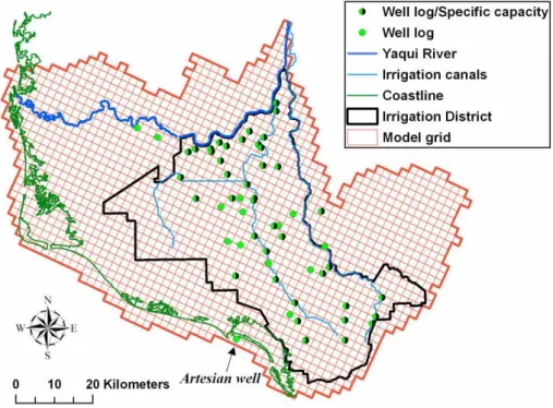
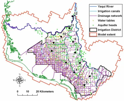
Fig. 1.Location of the Yaqui Valley study area, the Yaqui Irrigation District, and extent of the groundwater model.
within a single optimization run (Gupta et al., 2003). These Pareto solutions explicitly represent trade-offs between the various objectives. The advantage is that no prior weights need to be assigned to the different objectives, since they are treated independently (Schoups et al., 2005). In addi-tion, the multi-objective approach includes more information about the hydrologic system in the parameter identification process, thereby potentially leading to better estimates of the parameters (Boyle et al., 2000). On the other hand, signifi-cant trade-offs in fitting two or more objectives may indicate an error in the model structure (Refsgaard and Henriksen, 2004), for example a relevant physical process may not be accounted for or it may be wrongly parameterized.
This paper discusses the application of a multi-objective global optimization approach to the calibration of a regional surface water-groundwater flow model. The study area is the 6800 km2Yaqui Valley in the state of Sonora, one of the most important agricultural regions in Mexico. Irrigated agricul-ture in the Yaqui Valley has since 1942 relied on the supply of water from surface reservoirs. A recent prolonged eight year drought (1996–2004) however has drawn down these reser-voir levels below sustainable levels, resulting in severe cuts in water supply and widespread fallowing (Addams, 2004). For the first time in 40 years, due to the effects of the drought on reservoir depletion, wheat was not grown in Yaqui Valley, which is the center for the “Green Revolution” for wheat in
Mexico. Due to uncertainties in the future supply of surface water for irrigation, farmers in the Yaqui Valley will depend more and more on groundwater as an additional or even pri-mary source of irrigation water.
The integrated surface water-groundwater model pre-sented here revises the original model of Addams (2004) and serves as a first step to developing a comprehensive water management plan for the region. Unlike previous hydrogeo-logic research in the Yaqui Valley (Diaz, 1995; Islas, 1998; Steinich and Chavarria, 2000), the flow model presented here incorporates all known spatially distributed stresses on the system, including pumping, drainage, irrigation canal seep-age, and field irrigation losses (Addams, 2004). Using hy-draulic heads, canal seepage rates, and drainage volumes, a multi-objective calibration problem is formulated and solved using the recently developed Multi-Objective Shuffled Com-plex Evolution Metropolis (MOSCEM-UA) global optimiza-tion algorithm of Vrugt et al. (2003b).
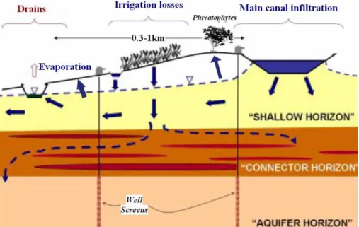
Fig. 2.Conceptual model of the Yaqui Valley surface water-groundwater system.
detail, highlighting the advantages of this approach com-pared to more traditional methods and summarizing insights into the regional flow system of the Yaqui Valley.
2 Methods
2.1 Study area: water resources and hydrogeology
Figure 1 shows the location of the Yaqui Valley, which lies between the coastal plain of the Sea of Cortez to the south-west and the Sierra Madre Mountains to the northeast. The climate is semi-arid with an average annual precipitation of ∼300 mm, most of it falling in the summer from June to September. Annual potential evapotranspiration averages 2000 mm. Most of the farmland in the Valley is part of the Yaqui Irrigation District (Fig. 1). The dominant crop is win-ter wheat, which is grown from November to April, and is irrigated using a combination of surface water and ground-water. The surface water system consists of three reservoirs in series on the Yaqui River, the largest and furthest down-stream being the Oviachic reservoir (Fig. 1). Surface water releases from Oviachic reservoir are conveyed to the Yaqui Irrigation District by means of open unlined canals. Along the way, water is diverted by the various agricultural water management units, known as modules, that make up the Ir-rigation District. Water is further distributed to individual fields within each module by means of a network of sec-ondary irrigation canals. Almost 600 wells have also been installed (Fig. 1) to provide additional water for crop pro-duction, although these are never all active in the same year. Some of the wells are privately operated whereas others are managed by the District. Throughout the Irrigation District,
a drainage network has been installed to drain surplus irriga-tion water from fields out to the Sea of Cortez. These drains are primarily open drainage ditches, with a small percentage of subsurface drainage pipes, at a depth of 1 to 2 m below the land surface. Most of the soils in the valley are clayey verti-sols with organic matter contents less than 1% (Lobell et al., 2002).
Fig. 3.Locations of wells with well log and specific capacity data used to define model layers and hydraulic properties. The model grid is also shown.
and underlying older unconsolidated Tertiary deposits. De-pending on the magnitude of the contrast in hydraulic con-ductivity with the overlying confining layer, the deep aquifer behaves either as a confined, semi-confined, or unconfined system. Addams (2004) provides more details on how layer geometry was determined for modeling purposes.
An estimate of the available storage in the deep aquifer under the Irrigation District is made by summing the avail-able storage under confined conditions (above the top of the screened wells), assuming a specific storage of 10−4m−1,
plus the remaining storage under unconfined conditions, as-suming a specific yield of 0.2 and counting 2/3 of the aquifer thickness. This results in a value of approximately 100 000 MCM (Million Cubic Meters), which is about 16 times the available storage in the Yaqui reservoir system (6000 MCM). In addition, the supply of surface water is variable and uncer-tain as was evident during the recent drought. Hence, avail-able water in the deep aquifer will likely play a central role in a sustainable water management plan in the Yaqui Val-ley. Historically, groundwater use has been limited due to the availability of cheap surface water and the relatively high cost of pumping.
2.2 Hydrologic model
In this section, we discuss the concepts and methods used to simulate flow in the integrated surface water-groundwater system of the Yaqui Valley. For further details we refer to Addams (2004). Special attention is paid to representation
of the near-surface hydrologic processes, such as recharge, evaporation, and near-surface drainage, and to the coupling between the surface water and groundwater systems. To re-duce uncertainty, we independently estimate as many param-eters as possible (e.g., recharge), and then find optimal values for the remaining parameters.
The groundwater component of the flow model was repre-sented using the transient 3-D groundwater flow equation,
∂ ∂x
Kx
∂h ∂x
+ ∂ ∂y
Ky
∂h ∂y
+ ∂ ∂z
Kz
∂h ∂z
−W=Ss
∂h ∂t
, (1)
whereKx, Ky, andKz are hydraulic conductivity values in
the x, y, and z direction [L/T], h is hydraulic head [L], t is time [T], W is a source-sink term [1/T] representing recharge, pumping, evaporation, or drainage, andSs is
spe-cific storage [1/L], which when multiplied by the saturated thickness gives the confined aquifer storage coefficient,S[-], or the unconfined aquifer specific yieldSy[-]. Groundwater
flow was simulated using Modflow-2000 (Harbaugh et al., 2000). The surface water component was simulated using a routing model for flow in the main irrigation canals, includ-ing a sink-source term representinclud-ing water exchange between the canals and the groundwater system (Prudic et al., 2004). 2.2.1 Spatial and temporal discretization
northeast and southwest. The model domain was discretized into a regular finite difference grid of three layers, each con-taining 60 rows and 70 columns, resulting in a total of 12 600 cells with an area of 2×2 km2each. This level of horizon-tal discretization is deemed sufficient, since the interest is in characterizing the regional flow system rather than account-ing for flow near individual wells. Cell thicknesses range from 5 to 170 m. The grid was oriented at a 25◦ azimuth angle to align it with the principal direction of groundwater flow from northwest to southeast. There were 5,064 active cells within the model boundaries shown in Fig. 1.
In the vertical direction, the three layers represented the shallow aquifer, confining layer, and deep aquifer as dis-cussed earlier. The top of the first layer coincides with the land surface elevation, which was determined from a Digi-tal Elevation Model (DEM) and a paper elevation map ob-tained from the National Water Commission (CNA) in Mex-ico. The bottom of the first layer, which is also the top of the second layer, was estimated by interpolating elevations from selected well logs (Fig. 3) each of which exhibits a change from coarse-grained to fine-grained material. Sim-ilarly, the top of the third layer corresponds to a transition from fine-grained to coarse-grained material observed in well logs. This transition also often coincided with the top of the well screen. Finally, the thickness of the third layer was de-fined as twice the well screen lengths, giving thicknesses of approximately 30 to 170 m. As such, the third layer rep-resents the approximate aquifer thickness of the productive aquifer material, rather than the total permeable thickness, which extends deeper as evidenced by geophysical measure-ments (Steinich and Chavarria, 2000).
The calibration period extends over 24 years, starting in October 1973 and ending in September 1997, corresponding to crop years 1974–1997. This period was selected for cal-ibration because it covers a long record of observed aquifer head data, including periods of increased groundwater pump-ing, as well as a period of measured rates of agricultural drainage (1988–1997). Since our primary interest is in the long-term response of the groundwater system, the entire simulation period was discretized into 24 annual stress pe-riods for which average annual boundary conditions were specified. Each stress period was divided into 10 time steps, using a fixed time step multiplier equal to 1.2. At the start of each annual stress period the initial time step in the model is initially on the order of a week and increases each time step by a factor of 1.2 throughout the year. The model was tested with much smaller time steps (using initial time steps less than 1 s) and essentially the same results were obtained for the simulated water balance and aquifer heads. In addition, water balance errors were always less than 0.01%. There-fore, the degree of temporal discretization was sufficiently accurate and led to reasonable computational times for the 3000 calibration simulations.
2.2.2 Initial conditions
Initial values for hydraulic heads were estimated by running the model at steady-state using time-averaged boundary con-ditions for the period 1972–1974 when data show that heads in the deep aquifer, pumping rates, and reservoir releases were all relatively constant. The head distribution from the steady-state model was then used as initial condition for the transient run from 1974 to 1997.
2.2.3 Irrigation, crop ET, and recharge
Recharge from field-scale irrigations is independently esti-mated using a mass-balance calculated each year and for each module in the Irrigation District,
R=SW+GW−ETc, (2)
whereRis annual recharge [L/T],SWis surface water deliv-ery to the module (includes conveyance losses during trans-port of water from the main irrigation canals to the fields) [L/T], GW is irrigation using groundwater [L/T], and ETc
is annual crop ET [L/T]. Annual rates of surface-water irri-gation delivered to the entire Yaqui Irriirri-gation District were distributed over the modules assuming that the spatial distri-bution of surface-water allocation was the same as that dur-ing the period 1996–1999 when module specific data were available. Annual groundwater pumping rates were avail-able for each well throughout the entire calibration period. Total groundwater irrigation within each module was esti-mated by calculating total pumping from all wells located within that module, excluding those wells that discharge di-rectly into the main irrigation canals. Finally, district-wide crop ET was estimated from annual crop acreage data and local crop water demand values (Addams, 2004). The main crop is winter wheat (50% of planted acreage), but a variety of other crops are grown as well, including soybeans, maize, cotton, safflower, and various vegetable crops. Estimates of annual consumptive use for these crops were obtained from local sources (CNA; Ortiz-Monasterio, personal communi-cation, 2001). The total crop ET was then distributed over the modules assuming the same spatial distribution as ob-served for the period 1996–1999. Note that the recharge val-ues calculated with Eq. (2) include recharge from irrigation water applied at the field-scale, as well as conveyance losses through the secondary irrigation canals, which distribute wa-ter from discharge points on the main irrigation canals to the fields. Average annual volumes of surface-water use, groundwater use, and crop water demand (consumptive use) for the period 1974–1997 were 2065, 271, and 1512 MCM, respectively. For further details of the spatial treatment of irrigation-related recharge and crop ET, see Addams (2004). 2.2.4 Canal seepage
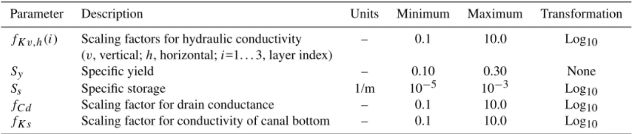
Table 1.Calibration parameters and their prior uncertainty ranges.
Parameter Description Units Minimum Maximum Transformation
fKv,h(i) Scaling factors for hydraulic conductivity – 0.1 10.0 Log10
(v, vertical;h, horizontal;i=1. . . 3, layer index)
Sy Specific yield – 0.10 0.30 None
Ss Specific storage 1/m 10−5 10−3 Log10
fCd Scaling factor for drain conductance – 0.1 10.0 Log10
fKs Scaling factor for conductivity of canal bottom – 0.1 10.0 Log10
groundwater before canal water reaches the end of the canals. Canal volumetric seepage rates are simulated by discretizing the main canals into 145 reaches with inflow of surface water from the Oviachic reservoir (Fig. 1) specified annually at the head of each canal. Water is then routed through the canals using a water budget for each reach,
Qout=Qin+Qgw−Qsw−Qseep, (3)
whereQoutis outflow from the reach [L3/T],Qinis inflow
into the reach [L3/T], Qgw represents pumping of
ground-water into the canal [L3/T],Q
sw is diversion of surface
wa-ter for irrigation [L3/T], andQseepis canal seepage into the
aquifer [L3/T]. Direct evaporation from the canals consti-tuted less than 0.5% of the monthly seepage losses and was neglected. Additions to each canal reach by groundwater pumping,Qgw, are estimated from annual CNA records of
well-specific pumping, whereas water diversions to the agri-cultural modules are calculated from annual surface water use in each module,SW in Eq. (2), and the location of its diversion points along the canals. The canal-groundwater in-teraction term,Qseep, is calculated using Darcy’s law, Qseep=
KswsLs
ms
(hs−h) for h≥hbot, (4a)
Qseep= KswsLs ms
(hs−hbot) for h < hbot, (4b)
whereKs is hydraulic conductivity of the canal bed [L/T],
ws is canal width [L],Ls is canal length [L], ms is
thick-ness of the canal bed [L],hs is head in the canal reach [L],
hbotis elevation of the canal bed bottom [L], andhis head in
the underlying water table aquifer [L]. For each canal reach, values forws andLs were estimated from District records,
andmswas set at a uniform value of 0.1 m. The elevation of
the canal bottom was defined relative to the land surface el-evation. However, due to the coarse spatial resolution of the groundwater model (grid cells of 2 by 2 km), the elevation of the canal bottom was specified higher than the average land surface elevation of the grid cell in areas of steeper topog-raphy near the mountain front (Fig. 1). Uniform initial val-ues forKsequal to 0.014 and 0.01 m/yr were estimated from
data on canal seepage rates and estimated water depths in the
canals, whereas the lined yet leaky parts of the canal were assigned an initialKs of 0.001 m/yr. Due to the uncertainty
on the values ofKs, the initial estimates were multiplied by a
scaling factor,fKs [-], which was subject to calibration
(Ta-ble 1). Heads,hs, or water depths,ds=hs−hbot−ms, in the
canals are calculated using the following approximation to Manning’s equation for a 45◦trapezoidal cross-section, ds =b
p
Qs, (5)
where ds is water depth [L],Qs is flow at the midpoint of
the canal reach [L3/T], andbis a coefficient [(L/T)−0.5]
es-timated as a function of roughnessn, slopeS, and widthws
of each canal reach (Addams, 2004). The canal-aquifer sys-tem represented by Eqs. (1), (3), and (5) interacts through the seepage term in Eq. (4), requiring an iterative solution at each time step. The system was solved using the stream package of Prudic et al. (2004) and Modflow (Harbaugh et al., 2000). 2.2.5 Recharge outside the Irrigation District
Outside the Irrigation District there are three additional sources of recharge to groundwater: recharge from irriga-tion in the Yaqui Colonies, Yaqui River infiltrairriga-tion, and mountain-front recharge. The Yaqui Colonies, tribal lands located to the north of the Irrigation District, have a perpetual right to approximately 250 MCM/yr of surface water, which was estimated to result in a constant uniform recharge rate of 0.37 m/yr based on the assumption of recharge mechanisms similar to the District. Yaqui River infiltration upstream of the irrigation canals (Fig. 1) was calculated annually from tabulated Irrigation District data. Except in extremely wet conditions, no water flows in the Yaqui River past the in-take of the irrigation canals (Addams, 2004). Precipitation is only a significant source of recharge near the mountain-front boundaries (Fig. 1). This mountain-mountain-front recharge was estimated as (Anderson et al., 1992),
log10(Qmfr)= −1.34+log10(P ) , (6) where Qmfr is the volume of mountain-front recharge
recharge is dampened by slow unsaturated zone percolation (Flint et al., 2000). Therefore, long-term average precipi-tation at the Oviachic Reservoir (0.2 m/year) was used for P, resulting in constant recharge rates of 0.03 m/year and 0.04 m/year for the Bacatete and Baroyeca mountain fronts, respectively. Direct precipitation in the valley was neglected as a source of recharge in this semi-arid climate with summer temperatures that reach 40◦C.
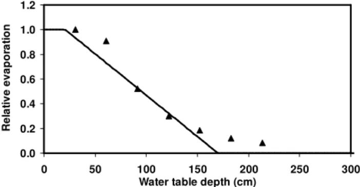
2.2.6 Non-agricultural ET and bare soil evaporation In addition to crop evapotranspiration, one also needs to ac-count for evaporation from native and riparian vegetation along the irrigation canals and near the coast, as well as bare soil evaporation after the crop growing season. Annual po-tential evaporation averages 2 m/yr, approximately 60% or 1.2 m of which occurs from May to October, i.e., after the main wheat growing season. Actual evaporation rates are limited by the availability of moisture near the soil surface, which mainly depends on the soil hydraulic properties and the water table depth (Gardner, 1958; Gardner and Fireman, 1958). Hypothetical analysis of evaporation for a clay soil, which is the main soil type in the area, as a function of wa-ter table depth was estimated using Hydrus ( ˇSim˚unek et al., 1998). Results suggest an approximate linear relation be-tween relative evaporation, i.e. the ratio bebe-tween actual and potential evaporation, and water table depth, as shown in Fig. 4. Maximum evaporation rates occur when the water table is within 0.2 m of the land surface and no evapora-tion takes place when the water table approaches 2 m depth. These values were used to calculate evaporation as a func-tion of water table depth. Maximum evaporafunc-tion rate was set at 2 m/yr outside the Irrigation District. Inside the Dis-trict consumptive use by crops during the growing season is already accounted for in Eq. (2), hence the potential evapora-tion rate was set at 1.2 m/yr. Although this neglects any addi-tional evaporation that may occur during the growing season, the simulations indicated that the upper limit of 1.2 m/yr was typically not reached within the District. A linear approxima-tion was applied by fitting to the “data” points from Hydrus and then calculating the relative evaporation as a function of water table depth (Fig. 4).
2.2.7 Water table drainage through drainage network Throughout the irrigation district, a drainage network has been installed to keep the water table from rising to the ground surface. The network drains (Fig. 5) surplus irriga-tion water from fields out to the Sea of Cortez. These drains consist partly of open drainage ditches, and partly of subsur-face drainage pipes. In the model, groundwater flow to drains is simulated as a linear head-dependent sink,
Qd =LdCd[h−hd] (7)
whereQdis drain flow [L3/T],Ld is total drain length [L],
Cd is drain conductance [L/T], hd is drain elevation [L],
0.0 0.2 0.4 0.6 0.8 1.0 1.2
0 50 100 150 200 250 300
Water table depth (cm)
R e la ti v e e v a p o ra ti o n
Fig. 4.Relation between relative evaporation and water table depth for a clay soil, simulated with the HYDRUS code (triangles) and approximated with a piecewise linear function.
andh is hydraulic head in the grid cell [L]. The total drain length,Ld, in each grid cell was determined by overlaying
the drainage network map onto the model grid. Drain ele-vations,hd, for each drain segment were determined from
land surface elevations and assuming a uniform drain depth of 2 m. Finally, drain conductance values, Cd, were
esti-mated using monthly observed drainage volumes and water table elevations from January 1996 to September 1997 for 13 sub-areas. These initialCd values were multiplied by a
uni-form scaling factor,fCd[-], which was subject to calibration
(Table 1).
2.2.8 Groundwater pumping
Annual well pumping data were gathered from CNA sources for a total of 591 wells (Fig. 1), although only a part of these are active in any given year. All pumping was assigned to the main aquifer, i.e. layer 3.
2.2.9 Boundary conditions
The bottom boundary of the model domain approximately corresponds to the deepest extent below which groundwa-ter flow in the deep aquifer is not influenced by agricultural pumping. Hence, a zero-gradient boundary condition was used at the bottom boundary, which prevents any water from leaving or entering the model through the bottom.
Fig. 5. Locations of wells with observed water table elevations and aquifer heads used for model calibration. The drainage networks with measured drainage volumes are also shown. Numbers correspond to wells for which time-series are shown in Fig. 14.
the model there as well. Finally, the southwest offshore boundary parallels the shoreline and is simulated as a con-stant head boundary, with heads set equal to zero (sea level) in the uppermost layer, allowing water to leave or enter the domain through that layer. However, no-flow boundaries are assumed for the second and third layers along the offshore boundary to simulate artesian conditions observed in an off-shore island well (Fig. 3). Because discharge of groundwater occurs beneath the Sea of Cortez, it was important that the model reproduce the head value in this offshore island well because it constrains the degree of submarine confinement of the aquifer. Vertical hydraulic conductivity in other locations along the coastline was high enough to enable deep ground-water discharge into the Sea of Cortez through the constant-head boundary of the upper layer.
2.2.10 Hydraulic properties
The spatial distribution of horizontal (Kh)and vertical (Kv)
hydraulic conductivities was estimated from lithologic data and well tests. It was assumed that the aquifer is horizon-tally isotropic in each layer but vertically anisotropic, hence Kx=Ky=Kh, and Kz=Kv. For the deep aquifer, specific
capacity values were calculated for 41 wells with pumping rates, static head levels, and dynamic pumping head levels recorded at the time of drilling (Fig. 3). These specific ca-pacity values were converted into transmissivity values
us-ing the followus-ing empirical relationship (Razack and Hunt-ley, 1991),
T =15.3 S0c.67 (8)
whereT is transmissivity andScis specific capacity, both in
units of m2/day. Since the permeable formation extends for some distance beneath the bottom of the well screen, corre-sponding values forKhwere estimated as,
Kh3= T2b (9)
wherebis the well screen length [L]. The resultingKh3
val-ues were interpolated to the model grid. Finally, initial valval-ues of vertical hydraulic conductivityKvwere estimated to be an
order of magnitude smaller than the correspondingKh3
val-ues, i.e.Kv3=Kh3/10.
estimate of the spatial distribution of hydraulic conductivity. The spatial distribution ofKhin layer 1 was estimated as,
Kh1= 101−x (10)
where x is the interpolated clay fractional thickness (0–1), resulting in values for Kh1 between 1 and 10 m/day. A
hydrogeologically reasonable estimate of 10:1 was adopted for the uncalibrated vertical anisotropy ratio in layer 1, or Kv1=Kh1/10. Finally, for layer 2 the vertical hydraulic
con-ductivity was first estimated as,
Kv2= 10−ay (11)
where y is the interpolated clay thickness (0–50 m). The value ofawas set to 0.1 in order to reproduce artesian con-ditions observed in the offshore well in Fig. 3. This results in initial estimates forKv2between 10−5and 1 m/day.
Hor-izontal hydraulic conductivity in the layer was estimated us-ing a 10:1 anisotropy ratio, henceKh2=10Kv2.
Given the uncertainty of these initial estimates, theKvand
Kh values in each layer were scaled by factors, fKvi and
fKhi, whereiis the layer index. These six scaling factors
were subject to calibration (Table 1). Finally, spatially uni-form values for specific yield,Sy[-], and specific storage,Ss
[1/L], were also estimated by calibration. 2.3 Parameter optimization
2.3.1 Calibration parameters and targets
A total of 10 parameters were subject to calibration, as listed in Table 1. For each parameter a reasonable physical prior range of values was specified centered around the initial es-timates discussed in the previous section. The model is cal-ibrated using data on water table elevations, aquifer heads, drainage volumes, and canal seepage volumes for the period 1974–1997. Figure 5 shows the well locations with water ta-ble and aquifer head observations during this period. Note however that every well doesn’t necessarily have a measure-ment each year. Water table measuremeasure-ments in September are compared to simulated values at the end of each annual stress period. Aquifer heads are measured annually in October, when wells were turned off for 1–2 days prior to measure-ment and when almost no pumping occurs since the main growing season is from November to April. These measure-ments are compared to simulated heads at the end of each annual stress period. Since annually averaged groundwa-ter pumping is used in the model, this implicitly assumes that the head at the end of the water year is not affected by intra-annual pumping changes. The third data set used for calibration consists of annual drainage rates in the agricul-tural drainage network (Fig. 5) during 1988–1997 measured at various discharge locations near the Sea of Cortez. Finally, the Irrigation District also maintained records of the total an-nual volume of surface water lost by seepage from the main
canals during 1974–1997. Those values were compared to the corresponding simulated volumes.
Since there are four different types of data to calibrate to, we can formulate four independent root mean square error objective functions,
RMSEk=
v u u t 1 nk nk X
i=1
ψk,OBS(i)−ψk,SIM(i)2 (12)
wherekindicates the type of measurement (water table “wt”, aquifer head “aq”, drainage volume “drain”, and canal seep-age volume “seep”), RMSEk is the root mean square error
for data typek,nk is the number of measurements for data
typek (891, 3506, 130, and 48 respectively for “wt”, “aq”, “drain”, and “seep”),ψk,OBS(i)is theith observation of data
typek, andψk,SIM(i)is the corresponding simulated value.
Ideally, we would like to identify an optimal parameter set that minimizes all four objective functions simultaneously. However, this is typically not possible due to errors in the conceptual model. Therefore, the trade-offs between match-ing the different objectives were investigated by performmatch-ing a multi-objective calibration and evaluating the tradeoff rela-tions in the Pareto optimal surfaces.
2.3.2 Calibration algorithm
The goal of the multi-objective optimization is to minimize F (p)= hf1(p), f2(p), ..., fN(p)iwith respect top, where
Fis the vector of objectives,fk(p) is thekth objective
func-tion in Eq. (1), andpis a vector of model parameters (Gupta et al., 2003). The solution to this problem will not be a sin-gle “best” parameter set, but will consist of a Pareto optimal set of solutions corresponding to trade-offs among the objec-tives. Formally, the Pareto set consists of parameter com-binationspi with the following properties: (1) for all
non-memberspn there exists at least one memberpi that
dom-inates pn, and (2) it is not possible to find another
mem-ber pj within the Pareto set that dominates pi. By
defi-nition,pi dominates pj if, for allk,fk(pi)<fk(pj). Our
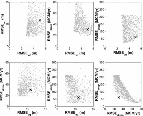
Fig. 6.Bi-criterion plots for the four-objective calibration run after 3000 model evaluations with the MOSCEM-UA algorithm.
dominated and non-dominated points. The non-dominated parameter setsiare assigned a fitness valueri,
ri =
ni
s (13)
whereni is the number of parameter sets dominated by
pa-rameter seti. The dominated parameter setsj on the other hand are assigned a fitnessrj,
rj =1+
X
i≤j
ri (14)
where the summation is over all parameter setsithat dom-inate parameter setj. Parameter sets with low fitness val-ues are retained, resulting in a preference of non-dominated parameter sets at the extremes of the Pareto front. This strategy prevents convergence in the compromise region of the objectives. The algorithm proceeds by dividing the ini-tial parameter populationsinto a number of so-called com-plexes. Within each complex new parameter sets are gener-ated by sampling from a multi-normal distribution estimgener-ated from all points in the complex, and new points are accepted or rejected based on their fitness value. After a prescribed number of iterations, all parameter sets are shuffled and new complexes are formed. Repeated application of these steps causes the population to converge to the Pareto set of so-lutions. The Pareto parameter set also contains the single objective solutions at the extremes of the Pareto solution set (end-members). Therefore, using one optimization run the
MOSCEM-UA algorithm generates all information needed to evaluate best parameter values for each data type (see Vrugt et al., 2003b).
Here the MOSCEM-UA algorithm was run with an initial populationsof 200 parameter sets (sets of 10 parameters), randomly selected from the prior ranges defined in Table 1. This initial sample set was then divided into 5 complexes for subsequent optimization for a total of 3000 model simula-tions or evaluasimula-tions.
3 Results and discussion
Fig. 7.Bi-criterion plots for the four-objective calibration run after 3000 model evaluations with the MOSCEM-UA algorithm, without bare soil evaporation.
3.1 Four-objective calibration
Figure 6 presents bi-criterion plots for the four-objective cal-ibration after 3000 model evaluations with the MOSCEM-UA algorithm. Each plot is a marginal multi-objective curve showing two criteria out of four total criteria dimensions. Each dot represents one forward simulation of the groundwa-ter model. The large cross indicates the simulation that yields the minimum distance in the four-dimensional normalized objective function space. Two observations are made based on these plots. First, from the first three plots in Fig. 6 it can be seen that there is very little variation in the RMSEwt for
the range of parameter values considered here (Table 1). This indicates that the simulation of water table elevations is quite insensitive to any of the parameters. This may be explained by the fact that the shallow water tables in the model are con-trolled by drainage in the engineered agricultural drains and evaporation, which tend to control and suppress large vari-ations in simulated water table elevvari-ations. Second, the re-maining bi-criterion plots that do not involve RMSEwt
(bot-tom three plots in Fig. 6), all exhibit trade-offs along a right angle. This indicates that improvements in fitting one ob-jective can be made without deteriorating the fit to the other objective. In other words, these results suggest that there is little trade-off between fitting the different objectives, and that they can be considered independently. The absence of
any significant trade-offs indicates that the model is gener-ally well conceptualized, and that most relevant hydrologic processes are accounted for.
At this point it is useful to consider the effect of bare-soil evaporation on the results of the multi-objective optimiza-tion, particularly since the initial groundwater model concep-tualization did not include bare soil evaporation as a signif-icant physical process (Addams, 2004). Figure 7 shows the same plots as Fig. 6, but now bare soil evaporation was omit-ted. The main differences are that (1) without evaporation there is much more scatter in the plots involving RMSEwt
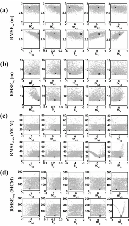
Fig. 8.Dotty plots for the four-objective calibration run, showing sensitivity of the various objective functions to the calibration parameters.
(a)water table elevations,(b)aquifer heads,(c)drainage rates, and(d)canal seepage rates. All parameter scales are log-transformed, except
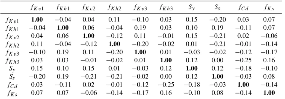
Table 2.Parameter correlation coefficient matrix for a subset of simulations, identified by the following criteria: RMSEwt<3, RMSEaq<10,
RMSEdrain<30, and RMSEseep<50.
fKv1 fKh1 fKv2 fKh2 fKv3 fKh3 Sy Ss fCd fKs
fKv1 1.00 −0.04 0.04 0.11 −0.10 0.03 0.15 −0.20 0.03 0.07 fKh1 −0.04 1.00 0.06 −0.04 0.19 0.03 0.10 0.19 −0.11 0.07 fKv2 0.04 0.06 1.00 −0.12 0.11 −0.01 0.15 −0.21 0.02 −0.06 fKh2 0.11 −0.04 −0.12 1.00 −0.20 −0.02 0.01 −0.21 −0.01 −0.14
fKv3 −0.10 0.19 0.11 −0.20 1.00 0.01 −0.03 −0.02 −0.12 −0.17 fKh3 0.03 0.03 −0.01 −0.02 0.01 1.00 0.12 0.00 −0.25 0.16
Sy 0.15 0.10 0.15 0.01 −0.03 0.12 1.00 0.12 −0.18 −0.10
Ss −0.20 0.19 −0.21 −0.21 −0.02 0.00 0.12 1.00 −0.03 0.08
fCd 0.03 −0.11 0.02 −0.01 −0.12 −0.25 −0.18 −0.03 1.00 −0.14
fKs 0.07 0.07 −0.06 −0.14 −0.17 0.16 −0.10 0.08 −0.14 1.00
multi-objective optimization is a useful method for simulta-neously dealing with parameter and model structural uncer-tainty.
In the following paragraphs we investigate how well the model parameters are identified by the four objective func-tions. Figure 8 presents so-called dotty plots (Beven and Freer, 2001) for each of the four objectives (a–d) as a func-tion of each of the 10 calibrafunc-tion parameters. Note that all parameter scales on the horizontal axes are log-transformed, except forSy. Starting with the water table elevations, Fig. 8a
indicates that RMSEwtis relatively more sensitive to the
hor-izontal hydraulic conductivity of the deep aquifer,Kh3, and
the conductivity of the canal bottom, Ks, compared to the
other parameters. However, as discussed above, RMSEwt
is not sensitive to any of the parameters as evidenced by its small variation (around 2.5–3 m). Secondly, Fig. 8b shows that the simulated deep aquifer heads are most sensitive to the deep aquifer hydraulic conductivity, Kh3, and less
ob-viously the vertical hydraulic conductivity of the confining layer,Kv2. Best performance on aquifer heads, as indicated
by low values for RMSEaq, are obtained for fKh3 values
greater than 0. Hence, the multi-objective analysis shows that increases inKh3result in a better simulation of the aquifer
heads compared to using the initially estimated values for this parameter (which corresponds to fKh3=0). The minimum
value of RMSEaqidentified by the MOSCEM-UA algorithm
is 7.2 m (Fig. 8, Table 3). Figure 8b suggests that improve-ments in the simulation of aquifer heads may be possible by re-examining theKv2andKh3parameterizations. This will
be investigated in the next section. With regard to the sim-ulation of drainage rates, Fig. 8c clearly demonstrates that RMSEdrainmainly depends on the value of the drain
conduc-tances (fCd). On the other hand, RMSEseepis primarily
sen-sitive to the canal bed hydraulic conductivity,Ks (Fig. 8d).
Overall, the results in Fig. 8 suggest that the different objec-tives are sensitive to different parameters, implying that each objective could be fitted independently by finding the
opti-mum value(s) for its most sensitive parameter(s). This con-firms the conclusions that were drawn from Fig. 6 about the independence of the objective functions. It also means that the interaction between the surface water and groundwater systems is limited. We further conclude that improvements in the simulation of heads in the deep aquifer are most likely by reconsidering theKv2andKh3parameterizations, and this
could be done without significantly affecting the other three objectives.
It is important to realize that these findings most likely would have been obscured in a single-objective analysis, as the different data types would have been lumped into a sin-gle objective function, thereby blurring the sensitivity of the parameters to certain data types. Furthermore, the sensitivity and identifiability of the parameters would then essentially depend on the weights assigned to the different data types. Therefore, the independence of the different objectives in the multi-objective analysis increases the information content of the data and results in better parameter estimates.
What the dotty plots do not show is possible correlation between the parameters, which if present could cause poor parameter sensitivity and identifiability. Table 2 shows corre-lation coefficients between the 10 parameters based on a sub-set of simulations in the region of compromise of the four-objective space, identified by the following criteria: RMSEwt
<3, RMSEaq<10, RMSEdrain<30, and RMSEseep<50. Note
that these correlations were calculated on the estimates of the parameter values, not the log-transformed values. The strongest correlation in Table 2 equals−0.25, between pa-rameters fCd andfKs, suggesting that, for the sake of
pa-rameter identifiability, papa-rameter correlations are small (Hill, 1998).
Table 3.Optimal parameter and RMSE values for various objectives. “Euclid-dist” refers to the distance in the normalized four-dimensional objective function space.
Minimize Minimize Minimize Minimize Minimize RMSEwt RMSEaq RMSEdrain RMSEseep “Euclid-dist”
fKv1 2.9 3.3 1.1 4.3 0.6
fKh1 7.8 1.6 7.3 1.2 2.0
fKv2 0.4 1.1 0.4 0.5 0.2
fKh2 9.3 7.3 1.6 0.5 1.7
fKv3 0.4 8.4 1.2 0.5 0.4
fKh3 8.6 9.1 2.9 0.9 7.0
Sy 0.26 0.11 0.15 0.18 0.2
Ss 2.0E-04 1.8E-05 6.6E-05 3.3E-05 5.3E-04
fCd 0.1 5.1 1.7 2.4 1.8
fKs 0.6 0.4 0.9 1.3 1.3
RMSEwt(m) 2.5 2.6 2.8 2.9 2.8
RMSEaq(m) 7.4 7.2 9.4 15.5 7.7
RMSEdrain(MCM) 41.4 23.6 15.3 23.6 17.6
RMSEseep(MCM) 125.2 154.9 72.8 25.4 26.6
Fig. 9.Scatter plots of simulated versus observed water table eleva-tions, aquifer heads, drainage volumes, and canal seepage volumes.
values for the various objective functions is still quite large compared to the prior ranges specified in Table 1. In other words, the parameter uncertainty associated with the multi-objective Pareto solution is large, typically an order of mag-nitude. As was discussed earlier, this is due to the fact that the different objective functions are sensitive to different pa-rameters. However, this does not mean that the parameters are necessarily not well identified or that the model is in error. For example, canal seepage is very sensitive to the canal bed hydraulic conductivity (Fig. 8), hence this param-eter is known with certainty. Its Pareto uncertainty on the
other hand is large, because the other objectives are not that sensitive to it. Note also that the parameter values of the compromise solution usually lie close to the parameter value obtained by minimizing the objective function that is most sensitive to that parameter. For example, in the compromise solution, parameterfKs takes on the value of 1.3, which is
the same as its optimal value when fitting to the seepage rates only. The same can be said about parametersfCdandfKh3.
Furthermore, Table 3 shows that the compromise solution does only slightly worse in fitting the four objectives com-pared to the single objective results. Hence, little trade-off or compromise exists between fitting the four objective func-tions.
3.2 “Best” parameter set
Table 4.Time-averaged (1974–1997) water balance components in MCM for the different objective functions, as well as the compromise solution (minimum Euclidean distance). Negative numbers are groundwater sinks (outflows) and positive numbers are groundwater sources (inflows). An increase in storage is indicated by a negative number.
Minimize Minimize Minimize Minimize Minimize RMSEwt RMSEaq RMSEdrain RMSEseep “Euclid-dist”
Infiltration 2445 2445 2445 2445 2445
Canal seepage 233 159 338 463 454
Crop evapotranspiration −1513 −1513 −1513 −1513 −1513
Non-agricultural evapotranspiration −720 −272 −497 −490 −531
Drainage −86 −500 −421 −533 −448
Groundwater pumping −271 −271 −271 −271 −271
Groundwater discharge to Sea of Cortez −2 −18 16 8 −12
Change in groundwater storage −85 −29 −96 −107 −123
Figure 11 shows pie charts of the simulated time-averaged (1974–1997) annual water balance. The two main sources of water inflow into the groundwater system are, first, irri-gation water applied on agricultural fields and seepage from secondary irrigation canals, termed “infiltration“ in Fig. 11 (2445 MCM/year or 84% on average), and second, seepage from the main irrigation canals (454 MCM/year or 16%). Groundwater discharge is composed of crop evapotranspira-tion (1513 MCM/year or 53%), non-agricultural evapotran-spiration and bare-soil evaporation (531 MCM/year or 19%), surface and subsurface agricultural drainage discharging into the Sea of Cortez through the outlets of the drainage net-work (448 MCM/year or 15%), and groundwater pumping (271 MCM/year or 9%). Note that subsurface groundwa-ter discharge to the Sea of Cortez accounts only for 12 MCM/year which is less than 1% of the total annual out-flow. These simulated values compare well to observed canal seepage volumes (473 MCM/year on average) and drainage volumes (499 MCM/year observed on average during 1988– 1997, compared to 477 MCM/year simulated over the same period for that part of the drainage network that is moni-tored). In order to get a sense of the uncertainty of the sim-ulated water balance, Table 4 provides time-averaged wa-ter balances for the four objective functions of the multi-objective optimization. It is clear that most variation occurs in the drainage, evaporation, and canal seepage components. For example, when minimizing RMSEwt more water
dis-charges by evaporation (720 MCM) with very little drainage (86 MCM). Note that the compromise solution (minimum Euclidean distance) simulates a similar amount of drainage as the RMSEdrain objective, and a similar amount of canal
seepage as the RMSEseepobjective.
Finally, we investigated the model performance on aquifer heads using the best parameter set, and suggest an improve-ment in the model structure based on a spatial analysis of the model residuals. Figure 12a shows a map of the time-averaged residual error, interpolated from errors calculated
Fig. 10. Time-series of observed and simulated canal seepage and total drainage volume.
for the wells shown in the same figure. There are clear spatial patterns, with regions of consistent over-estimation (residual error greater than zero) and under-estimation (residual error smaller than zero). This suggests that some adjustment is needed in the spatial distribution of hydraulic properties, as initially estimated from well log and specific capacity data. Instead of using a single uniform scaling factor, we can use the spatial patterns in the model residual map to construct distinct zones of uniform scaling factors. This is discussed further in the next section.
3.3 Model refinement for aquifer heads
Fig. 11.Pie charts of the annual simulated water balance, averaged over the period 1974–1997 expressed as MCM and as percentages of the total inflows and outflows. Recharge below the root-zone, calculated as the difference between infiltration and crop ET, constitutes 65% of the total inflow into groundwater.
Table 5.Optimal parameter and RMSE values for various objectives. The different zones are mapped in Fig. 12b.
Zone Minimum (prior) Maximum (prior) Optimum Minimum* Maximum*
fKv2 1 0.01 100 1.0 0.08 9.4
2 0.01 100 0.01 0.01 0.19
3 0.01 100 37 6 97
4 0.01 100 0.013 0.01 0.15
fKh3 1 0.1 10 5 1.2 10
2 0.1 10 8.7 0.8 10
3 0.1 10 1.2 0.12 10
4 0.1 10 0.40 0.16 10
RMSEwt(m) 2.7
RMSEaq(m) 5.6
RMSEdrain(MCM) 17.4
RMSEseep(MCM) 26.2
* These are minimum and maximum values of all parameter sets with an RMSEaq<6 m.
drainage rates. However, results for the aquifer heads were less satisfactory as shown by the large value of RMSEaq(7.7
m) and the model residual map in Fig. 12a. Unfortunately, there is only limited information on the geology in this area. The available information (well logs) was used to specify the initial spatial distribution of conductivities, but there is con-siderable uncertainty on these estimates. Here an attempt is made to improve the model performance by including more (indirect) information about the geology, namely in the form of hydraulic heads in the deep aquifer. First, the spatial patterns in the model residual map were used to construct distinct zones of uniform scaling factors. This zonation is shown in Fig. 12b. Results from the multi-objective cali-bration also indicated that the simulation of aquifer heads is most sensitive to the scaling factors forKh3andKv2.
There-fore, the model was refined by introducing spatially varying scaling factors forKh3andKv2, defined by the zonation in
Fig. 12b. Based on the results of the multi-objective cali-bration run, changing these parameter values will have little effect on the simulation of water table elevations, drainage rates, and canal seepage rates.
A single-objective calibration was performed on aquifer heads only, using 8 calibration parameters, i.e. scaling fac-tors forKh3andKv2for each of the four zones in Fig. 12b.
All the other parameters that were considered before (Ta-ble 1) are now fixed at their “best” values as identified by the multi-objective calibration (Table 3). The SCEM-UA global optimization algorithm (Vrugt et al., 2003a) was used to identify the parameter values that minimize RMSEaq.
Fig. 12. (a)Interpolated map of time-averaged model residuals for simulated aquifer heads using the best parameter set of the multi-objective calibration,(b)corresponding zones of uniformKv2and Kh3scaling factors used in the single-objective calibration, and(c) resulting time-averaged residuals after the second calibration.
the zonation also caused a better fit to steady-state aquifer heads (1972–1974), as measured by a decrease in the steady-state RMSE values from 6.3 to 3.0 m. Values of the other
Fig. 13.Calibrated maps ofKv2(a)andKh3(b)using the optimal parameter set in Table 4 after the second calibration.
three objectives not included in the new calibration (Table 5) are similar, even slightly better, than those before the second calibration (Table 3). Nevertheless, spatial patterns in the model residuals still exist (Fig. 12c), although the errors have decreased. The optimal parameter values in Table 5 are con-sistent with the spatial patterns of over- and under-prediction in Fig. 12a. The over-predictions in zones 2 and 4 result in smaller values for fKv2 in these zones compared to the
best parameter set in Table 3, whereas the opposite occurs for zone 3, where heads were consistently under-predicted. Note that the scaling factors are again relative to the originally es-timated hydraulic conductivities using well log and specific capacity data. Although in Table 5, the optimal values of fKv2 for zones 2 and 4 are at or near the prior minimum
value of 0.01, the results could not be improved by letting fKv2reach even lower values. In other words, oncefKv2is
small enough very little water will percolate vertically. Final calibrated maps ofKv2andKh3, obtained by multiplying the
Fig. 14.Time-series of observed (triangles) and simulated (solid lines) aquifer heads for various locations, shown in Fig. 5. The dark solid line corresponds to the optimal solution of the single-objective calibration. The grey lines represent all simulations with an RMSEaqless
than 6 m.
Finally, parameter uncertainty was estimated on a set of behavioral models, defined by the criterion that RMSEaq<6 m. Minimum and maximum parameter values
for this subset of 229 parameter sets are shown in Table 5, and typically span an order of magnitude. The resulting pre-diction uncertainty is shown in Fig. 14. This figure presents time-series of observed and simulated aquifer heads for vari-ous locations, which are identified by a number in each graph corresponding to the numbered wells in Fig. 5. The opti-mal model is shown as a dark solid line, whereas the grey lines represent the range in prediction uncertainty associated with all parameter sets that result in an RMSEaq<6 m. In
most cases, the ranges in predicted heads bracket the obser-vations. Several simulated and observed heads decline dur-ing the 1970s and into the early 1980s, followed by a recov-ery in head levels after that. This corresponds to a period of increased groundwater pumping in the early 1980s, fol-lowed by an increase in surface water supply and a decrease in groundwater pumping after 1985.
4 Conclusions
is greater than the effects of parameter uncertainty, as evi-denced by a strong trade-off between the drainage and seep-age objectives when bare soil evaporation is not included in the model. Furthermore, by treating the different objectives independently, the method allowed for better identification of the model parameters compared to a single-objective ap-proach, since the various objectives were sensitive to differ-ent parameters. Large parameter variation (uncertainty) of the Pareto set of solutions, which includes the best-fit end-members for each of the objective functions, does not al-ways point to a model structural error, because such large parameter uncertainty may also be caused by the insensitiv-ity of one of the objectives for the parameter. The shape of the trade-off curve is a much better indicator of model struc-tural error. The simulated water balance shows that 15–20% of the water that enters the irrigation canals is lost by seep-age to groundwater. The main discharge mechanisms in the Valley are crop evapotranspiration (53%), non-agricultural evapotranspiration and bare soil evaporation (19%), surface drainage to the Sea of Cortez (15%), and groundwater pump-ing (9%). In comparison, groundwater discharge to the estu-ary was relatively insignificant (less than 1%). Heads in the deep aquifer were most sensitive to the vertical conductivity of the confining layer (Kv)and the horizontal conductivity
in the deep aquifer (Kh). The model was further refined by
identifying zonalKvandKhvalues based on a spatial
analy-sis of the model residuals. Subsequent calibration ofKvand
Khto aquifer head only (single-objective) resulted in further
improvements in simulated heads. Although the model was developed specifically for the Yaqui Valley, our results are relevant to other irrigated agricultural systems with shallow water tables. Future work will focus on an independent val-idation of the calibrated model, such that the model can be confidently used to identify optimal pumping strategies in the Yaqui Valley.
Acknowledgements. We would like to acknowledge data
con-tributions from the Yaqui Irrigation District and the Comisi´on Nacional del Agua in Mexico, as well as transcribed pumping data from S. Diaz and A. Canales at ITSON. We appreciate valuable insights from J.-L. Minjares and I. Ortiz-Monasterio. We would like to thank J. Vrugt for providing us with the MOSCEM-UA and SCEM-UA optimization algorithms. We are most grateful to the David and Lucile Packard Foundation for their support of this research. We are also grateful to the UPS Foundation for their support of the initial phases of this work.
Edited by: A. Gelfan
References
Addams, C. L.: Water resource policy evaluation using a combined hydrological-economic-agronomic modeling framework: Yaqui Valley, Sonora, Mexico, PhD-thesis, Stanford University, USA, 2004.
Anderson, T. W., Freethey, G. W., and Tucci, P.: Geohydrology and water resources of alluvial basins in south central Arizona and parts of adjacent states, USGS Professional Paper 1406-B, 1992. Beven, K. and Freer, J.: Equifinality, data assimilation, and uncer-tainty estimation in mechanistic modeling of complex environ-mental systems using the GLUE methodology, J. Hydrol., 249, 11–29, 2001.
Boyle, D. P., Gupta, H. V., and Sorooshian, S.: Toward improved calibration of hydrologic models: combining the strengths of manual and automatic methods, Water Resour. Res., 36, 3663– 3674, 2000.
Diaz, S.: Planeacion del uso conjunto de aguas superficiales y sub-terr´aneas en el Valle del Yaqui, Sonora: Modelaci´on del acu´ıfero del Valle del Yaqui, Instituto Technol´ogico de Sonora, Obregon, Mexico, 1995.
Doherty, J.: PEST, model-independent parameter estimation, Wa-termark Numerical Computing, Townsville, 2000.
Duan, Q., Gupta, V. K., and Sorooshian, S.: Effective and efficient global optimization for conceptual rainfall-runoff models, Water Resour. Res., 28, 1015–1031, 1992.
Flint, A. L., Flint, L. E., Hevesi, J. A., D’Agnese, F. D., and Faunt, C.: Estimation of regional recharge and travel time through the unsaturated zone in arid climates, in: Dynamics of fluids in frac-tured rock, edited by: Faybishenko, B., Witherspoon, P. A., and Benson, S. M., Am. Geophys. Union, 115–128, 2000.
Gardner, W. R.: Some steady state solutions of the unsaturated moisture flow equation with application to evaporation from a water table, Soil Sci., 85, 228–232, 1958.
Gardner, W. R. and Fireman, M.: Laboratory studies of evaporation from soil columns in the presence of a water table, Soil Sci., 85, 244–249, 1958.
Gonzales, R. and Marin, L. E.: Modelo Hidrogeol´ogico conceptual del acu´ıfero del Valle del Yaqui, Sonora en un contexto geol´ogico regional, Instituto Technol´ogico de Sonora, Obregon, Mexico, 2000.
Gupta, H. V., Bastidas, L., Vrugt, J. A., and Sorooshian, S.: Multi-ple criteria global optimization for watershed model calibration, in: Calibration of Watershed Models, edited by: Duan, Q., Am. Geophys. Union, Water Science and Applications Series, 6, 125– 132, 2003.
Harbaugh, A. W., Banta, E. R., Hill, M. C., and McDonald, M. G.: MODFLOW-2000, the U.S. Geological Survey modular ground-water model: User guide to modularization concepts and the Ground-Water Flow Process, USGS Open-File Report 00-92, 2000.
Hill, M. C.: Methods and guidelines for effective model calibration, USGS Water Resources Investigations Report 98-4005, 1998. Islas, L. A.: Determinaci´on y an´alisis espacial prospectivo de
las variables hidrodin´amicas del acu´ıfero del valle del Yaqui, Sonora, partiendo de informaci´on escasa, Instituto Technol´ogico de Sonora, Obregon, Mexico, 1998.
ITC: Geof´ısica integral del los Valles del Yaqui y del Mayo, Mexico City, 1979.
Lobell, D. B., Ortiz-Monasterio, J. I., Addams, C. L., and Asner, G. P.: Soil, climate, and management impacts on regional agri-cultural productivity from remote sensing, Agric. Forest Meteor., 114, 31–43, 2002.
objec-tives, Adv. Water Resour., 26, 205–216, 2003.
Poeter, E. P. and Hill, M. C.: Documentation of UCODE: A com-puter code for universal inverse modeling, USGS Water Re-sources Investigations Report 98-4080, 1998.
Prudic, D. E., Konikow, L. F., and Banta, E. R.: A new streamflow-routing package to simulate stream-aquifer interaction with MODFLOW-2000, USGS Open-File Report 2004-1042, 2004. Razack, M. and Huntley, D.: Assessing transmissivity from specific
capacity in a large and heterogeneous alluvial aquifer, Ground Water, 29, 856–861, 1991.
Refsgaard, J. C. and Henriksen, H. J.: Modeling guidelines, termi-nology and guiding principles, Adv. Water Resour., 27, 71–82, 2004.
Schoups, G., Hopmans, J. W., Young, C. A., Vrugt, J. A., and Wal-lender, W. W.: Multi-criteria optimization of a regional spatially-distributed subsurface water flow model, J. Hydrol., 311, 20–48, 2005.
ˇSim˚unek, J., ˇSejna, M., and van Genuchten, M. T.: The HYDRUS-1D software package for simulating the one-dimensional move-ment of water, heat, and multiple solutes in variably-saturated media, International Ground Water Modeling Center, Colorado School of Mines, 1998.
Steinich, B. and Chavarria, J. A.: Determination of hydrogeologi-cal characteristics and mapping of the sea water intrusion of the Yaqui Valley aquifer, Sonora, Mexico, in: Aquatic ecosystems of Mexico: status and scope, edited by: Munawar, M. L., Manawar, I. F., and Malley, D. F., Backhuys Publishers, Netherlands, 2000. Vrugt, J. A., Gupta, H. V., Bouten, W., and Sorooshian, S.: A Shuf-fled Complex Evolution Metropolis algorithm for optimization and uncertainty assessment of hydrological model parameters, Water Resour. Res., 39, 1201–1218, 2003a.