www.hydrol-earth-syst-sci.net/15/1547/2011/ doi:10.5194/hess-15-1547-2011
© Author(s) 2011. CC Attribution 3.0 License.
Earth System
Sciences
Increasing parameter certainty and data utility through
multi-objective calibration of a spatially distributed temperature
and solute model
C. Bandaragoda1and B. T. Neilson2
1Silver Tip Solutions, LLC., Mukilteo, WA, 98275, USA
2Utah Water Research Laboratory, Department of Civil and Environmental Engineering, Utah State University, Logan, UT, 84322, USA
Received: 4 October 2010 – Published in Hydrol. Earth Syst. Sci. Discuss.: 25 October 2010 Revised: 30 March 2011 – Accepted: 17 April 2011 – Published: 20 May 2011
Abstract. To support the goal of distributed hydrologic and instream model predictions based on physical processes, we explore multi-dimensional parameterization determined by a broad set of observations. We present a systematic approach to using various data types at spatially distributed locations to decrease parameter bounds sampled within calibration al-gorithms that ultimately provide information regarding the extent of individual processes represented within the model structure. Through the use of a simulation matrix, parameter sets are first locally optimized by fitting the respective data at one or two locations and then the best results are selected to resolve which parameter sets perform best at all locations, or globally. This approach is illustrated using the Two-Zone Temperature and Solute (TZTS) model for a case study in the Virgin River, Utah, USA, where temperature and solute tracer data were collected at multiple locations and zones within the river that represent the fate and transport of both heat and solute through the study reach. The result was a narrowed parameter space and increased parameter certainty which, based on our results, would not have been as suc-cessful if only single objective algorithms were used. We also found that the global optimum is best defined by multi-ple spatially distributed local optima, which supports the hy-pothesis that there is a discrete and narrowly bounded param-eter range that represents the processes controlling the dom-inant hydrologic responses. Further, we illustrate that the
Correspondence to:C. Bandaragoda ([email protected])
optimization process itself can be used to determine which observed responses and locations are most useful for esti-mating the parameters that result in a global fit to guide fu-ture data collection efforts.
1 Introduction
Typically the calibration of models involves fitting simula-tions to either single or multiple variables, error measures at a single location, or combining information from multiple locations (Duan, 2003). Early calibration techniques were notorious for converging to local optimal solutions and did not reliably find the global optimum (Schaake, 2003). Ad-ditionally, many hydrological modeling procedures do not make the best use of available information (Wagener et al., 2001). Current research on the calibration problem primarily focuses on uncertainty analysis and consideration of multi-ple objectives (Fu and Gomez-Hernandez, 2009; Blasone et al., 2008; Ajami et al., 2007; Duan et al., 2007; Vrugt and Robinson, 2007). Rather than selecting a single preferred parameter set, equifinality of models recognizes that there may be no single, correct set of parameter values for a given model and that different parameter sets may give acceptable model performance (Beven, 2001).
the model application, and the modeler. In this study, we consider a global optimum as the solution where there is ac-ceptable tradeoff between fitting the model at all locations there are data available, versus just matching data at one lo-cation well; this can be accomplished by using a range of multiple local optima defined by a narrowly bounded global optima. Since a model is not an exact representation of re-ality, and observed data used for verification are not perfect, the theoretical global optimum of a process based model dis-tributed in space and in time may be an unrealistic goal. However, a practical goal is to resolve the multiple local op-tima which simultaneously perform well on a local scale to narrowly bound the region surrounding the theoretical global optimum. In other words, there is a need to narrowly bound the global optimum region where good results exist for all data distributed throughout the system. Performing well lo-callyandglobally, or glocalization, can be used to define an optimum in model calibration which bridges scales between local and global performance. A systematic approach to us-ing various data types at spatially distributed locations to de-crease parameter bounds sampled within optimization algo-rithms is relevant to instream and hydrologic models ranging in application from the stream reach to the watershed scale.
The Two-Zone Temperature and Solute (TZTS) model (Neilson et al., 2010a,b) was developed to capture the domi-nant instream processes associated with heat and solute fate and transport. The TZTS model separates transient storage (Bencala and Walters, 1983) into two zones, (1) dead zones or the surface transient storage (STS) zone that represents the eddies, recirculating zones, and side pockets of water and (2) subsurface or hyporheic transient storage (HTS) zone, that represents the flow into or out of the stream substrate. As discussed in Neilson et al. (2010a), sources and sinks of heat include fluxes across the air-water interface, bed con-duction, conduction between the bed and deeper ground sub-strate, HTS exchange, and STS exchange. Solute mass is pri-marily influenced by HTS and STS exchange (Neilson et al., 2010b). To account for each of these fluxes, the TZTS model calculates energy and mass balances in the main channel, the STS zone, and the HTS zone for each reach or control vol-ume. As described further in Neilson et al. (2010a,b), the model equations are:
∂TMC
∂t = −UMC ∂TMC
∂x +D
∂2TMC ∂x2 +
Jatm ρCpYMC
(1)
+ αSTSYSTS Acs,MCβBtot
(TSTS −TMC)
+QHTS VMC
(THTS −TMC)
+ρsedCp,sedαsed ρCpYMCYHTS
(THTS −TMC)
dTSTS dt =
Jatm,STS ρCpYSTS
+ αSTS
(βBtot)2
(TMC −TSTS) (2)
+ρsedCp,sedαsed ρCpYSTSYHTS
TSTS,sed −TSTS
dTHTS dt =
ρCpQHTS ρsedCp,sedVHTS
(TMC−THTS) (3)
+ αsed YHTS2 (TMC
− THTS) + αsed YHTSYgr
Tgr −THTS
dTSTS,sed
dt =
αsed YHTS2 TSTS
−TSTS,sed
(4)
+ αsed YHTSYgr
Tgr −TSTS,sed
∂CMC
∂t = −UMC ∂CMC
∂x +D
∂2CMC
∂x2 (5)
+ αSTSYSTS Acs,MCβBtot
(CSTS− CMC)
+QHTS VMC
(CHTS −CMC)
dCSTS dt =
αSTS (βBtot)2
(CMC −CSTS) (6)
dCHTS dt =
QHTS (CMC −CHTS) YHTSAS,MC
(7) where T = temperature (◦C), Q= volumetric flow rate (m3s−1), V= zone volume (m3), D= longitudinal disper-sion (m2d−1),1x= volume length (m),αSTS= exchange be-tween the MC and the STS (m2d−1), QHTS= HTS advec-tive transport coefficient (m3d−1), Acs,MC= cross-sectional area of the MC (m2), Btot= total volume width (m), β= STS fraction of the total channel width, Y= volume depth (m), ρ= density of the water (g cm−3), Cp= specific heat of the water (cal g−1◦C−1), ρsed= density of the sed-iment (g cm−3), Cp,sed= specific heat of the sediment (cal g−1◦C−1),αsed= coefficient of thermal diffusivity of the sediment, and Jatm= atmospheric heat flux (cal cm−2d−1) (consisting of net shortwave radiation – 0.31 to 2.8 µm – at-mospheric longwave radiation – 5 to 25 µm – water long-wave radiation, conduction and convection, and evaporation and condensation), andC= concentration (mg L−1). The five subscripts (1) MC, (2) STS, (3) HTS, (4) STS, sed, and (5) gr, specify the main channel, surface transient storage, hyporheic transient storage, sediments below the STS and the deeper ground layer, respectively.
Fig. 1. Study reach layout including data collection locations. In-set map shows the state of Utah, USA, with the study area shown highlighted in black. (Taken directly from Bingham, 2010).
(e.g., within the main channel, HTS, and STS) at one loca-tion and longitudinally along a river segment, have created datasets that can be used to address the high dimensional problems associated with predicting heat and solute move-ment within streams and rivers. In recent studies (Neilson et al., 2010a,b), the TZTS model was calibrated using the Multi-Objective Shuffled Complex Evolution Metropolis al-gorithm (MOSCEM; see Vrugt et al., 2003a for alal-gorithm de-scription) and used to predict solute concentrations and tem-peratures in the Virgin River, Utah, USA, in storage zones at two different locations within the study reach. Using temper-ature and tracer observations at two different sites illustrated that using more spatially distributed information and two dif-ferent environmental tracers (temperature and solute) in the optimization improves the overall performance of the model. These studies found that even with the use of multi-objective calibration, many optimal parameter sets were indistinguish-able based on the objective functions, fairly broad parameter ranges resulted, and parameter uncertainty was still a con-cern.
In this paper, we address these issues by presenting a systematic approach to using various data types at spatially distributed locations to decrease parameter bounds sampled within optimization algorithms in the context of a case study. Our hypothesis is that there is a narrowly bounded parame-ter range that best represents the hydrologic processes con-trolling the system, which can be determined by using key data sets as multiple optimization objectives. To investigate this, we developed a simulation matrix of data types and sites that is used first to locally optimize parameter sets by fit-ting the respective main channel data using both single and
Fig. 2.Locations of temperature probes at Sites 2 and 3 within the study reach. (Taken directly from Neilson et al., 2010a).
multi-objective optimization algorithms. These results were then used to resolve which parameter sets perform best at in-dividual locations (distributed laterally and longitudinally) or have the best local fit, and which parameter sets result in the best global fit. Throughout this process we also test the util-ity of single and two-objective optimizations and determine the most informative calibration datasets resulting in global data fits.
2 Study area and data
A highly managed portion of the Virgin River, Utah, USA (Fig. 1), is considered impaired due to elevated temper-atures that have adversely affected two endangered fish species (Virgin River Chub – Gila seminuda, and woundfin – Plagopterus argentissimus) and other native fishes unique to this river system. An 11.94 km study reach of the Virgin River (Fig. 1) was divided into two main sections on the basis of bed slope (0.0039 between S1 and S2 and 0.0012 between S2 and S3) and stream substrate distribution identified from a previous mapping effort (Neilson et al., 2010a).
Corporation, Bourne, MA) with a±0.2◦C accuracy and res-olution of 0.02◦C.
Following methods also described in Neilson et al. (2010b), a 180 g instantaneous pulse of fluorescent Rho-damine WT dye was injected at 02:00:00 on 6 June 2007, at the head of a riffle just upstream of Site 1. A Self-Contained Underwater Fluorescence Apparatus (SCUFA) (Turner Designs, Sunnyvale, CA) was deployed in the main flow of the channel at both Site 2 and Site 3. Measurements were taken in situ every ten seconds for approximately 7 h at Site 2 and 6 h at Site 3. Grab samples were also collected at both Site 2 and 3 near the SCUFA to provide an independent measure in the main channel and in two representative STS locations. The grab samples were kept cool, stored in the dark in amber bottles with PTFE caps, and analyzed using a Turner Model 450 fluorometer (Turner Designs, Sunnyvale, CA). As discussed in Neilson et al. (2010b), loss of Rhodamine WT due to sorption to streambed sediments (mineral and organic) was not a concern in this study because the organic matter content in the bed sediments was extremely low (averaging 0.05 % at four sampling locations). Additionally, a recent sorption study within this portion of the Virgin River (Bingham, 2010) provided average Kd values of 1.5 mL g−1, which is low based on other Rhodamine WT sorption studies (Bencala and Walters, 1983; Everts and Kanwar, 1994; Lin et al., 2003; Shiau et al., 1993).
3 Methods
3.1 Simulation matrix
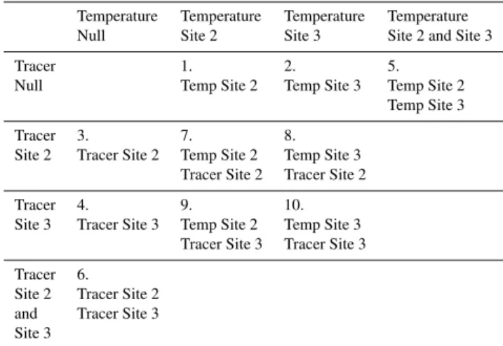
With the overall goal of iteratively reducing the size of the global search space, while simultaneously investigating the information content within the available data types, we es-tablished a simulation matrix (Table 1) to test the use of the most commonly collected main channel data sets used in cal-ibration of instream temperature and solute models. Each row and column denotes a data type that represents both tem-peratures and tracer concentrations at Site 2 and 3 along the study reach. This matrix represents all possible combinations of single and two-objective calibrations that use the available main channel temperature and tracer data. The calibration tests were Tests 1 through 4, which are single-objective cali-brations using main channel temperature and tracer at Site 2 and Site 3, and Tests 5 through 10 which are various com-binations of data resulting in two-objective optimizations. The latter two-objective tests include the following combina-tions: main channel temperatures at Site 2 and Site 3 (Test 5), main channel tracer observations at Site 2 and Site 3 (Test 6), main channel temperature and tracer observations at Site 2 (Test 7), main channel temperature at Site 3 and tracer obser-vations at Site 2 (Test 8), main channel temperature at Site 2
Table 1. Simulation matrix of ten single (1–4) and two-objective (5–10) calibrations combining main channel temperature and tracer observations at two locations (Site 2 and Site 3).
Temperature Temperature Temperature Temperature Null Site 2 Site 3 Site 2 and Site 3
Tracer 1. 2. 5.
Null Temp Site 2 Temp Site 3 Temp Site 2 Temp Site 3
Tracer 3. 7. 8.
Site 2 Tracer Site 2 Temp Site 2 Temp Site 3 Tracer Site 2 Tracer Site 2
Tracer 4. 9. 10.
Site 3 Tracer Site 3 Temp Site 2 Temp Site 3 Tracer Site 3 Tracer Site 3 Tracer 6.
Site 2 Tracer Site 2 and Tracer Site 3 Site 3
and tracer observations at Site 3 (Test 9), and main channel temperature and tracer observation at Site 3 (Test 10).
3.2 Calibration technique
sets. The HTS data were reserved for corroboration and test-ing of the model calibration. Since temperature and tracer data in the main channel are the most commonly collected data sets, we needed to further understand whether model calibration to main channel temperature and tracer data re-sults in realistic and representative STS and HTS predictions. Likewise, little was known about how single-objective model calibration at individual sites controls the resulting parame-terization at other site locations and for other data types. In addition to investigating how to narrow the optimization pa-rameter space, our methods are designed to test how a priori choices in study and project design, as well as data availabil-ity, may affect the model calibration and resulting simulation performance.
3.3 Model parameters
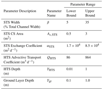
The a priori uniform distribution of the feasible parameter space was determined primarily based on earlier work that included a sensitivity analysis using Latin Hypercube sam-pling (Neilson et al., 2010a,b). For this study, these ranges were further expanded for some parameters based on pre-liminary optimization tests that resulted in parameter values consistently at the upper or lower bounds of their respective range (Table 2). The calibration parameters include: STS fraction of the total channel width (β), cross-sectional area of the STS (Acs,STS), exchange between the main channel and
the STS (αSTS), HTS advective transport coefficient (QHTS), and HTS depth (YHTS) for each of the two sections within the study reach (resulting in 10 parameters). The depth of the ground layer below the HTS (Ygr) was also estimated, but was represented by one value for both sections and be-came the eleventh calibration parameter. The total width of the main channel (Btot) and the Manning’s roughness coef-ficient (n), as required within the kinematic wave approach implemented within the TZTS model, were set based on the results of Bingham (2010). In this effort, multi-spectral and thermal imagery of the river system were used to physically estimate the average width of the channel over each section and therefore, reduced the number of parameters estimated in the calibration. WithBtotestablished,nwas then set to result in appropriate average travel times. The longitudinal disper-sion (D) coefficient was set based on the methods described in Neilson et al. (2010a).
3.4 Calibration objectives
To evaluate local and global model performance, various types of statistical measures were investigated. Each of the ten tests shown in Table 1 were run using different statisti-cal objectives including bias, Nash-Sutcliffe Efficiency (E), log error, and root-mean square error. Similar to Neilson et al. (2010a,b), we found thatE (Eq. 8; Nash and Sutcliffe, 1970) provided the most consistent calibration results and we
Table 2.A priori parameter range and calibrated parameter list for the TZTS model.
Parameter Range
Parameter Description Parameter Lower Upper Name Bound Bound
STS Width β 5 35 (% Total Channel Width)
STS CS Area Ac,STS 0.5 3
(m2)
STS Exchange Coefficient αSTS 1.7×10⁴ 8.5×10⁴
(m2d−1)
HTS Advective Transport QHTS 86 864
Coefficient (m3d−1)
HTS Depth YHTS 0.01 1
(m)
Ground Layer Depth Ygr 0.1 1.0
(m)
used this objective function throughout the remainder of the study and to quantify all local calibrations.
E = 1−
N
P
t=1
Tot −Tmt2
N
P
t=1 Tt
o −To 2
(8)
where, for N timesteps: Tot= observations, Tmt = modeled simulations (at time t), and To= mean of the observations. When used in calibration, the algorithm minimizes the result of 1−E, since the bounds ofEare [1,−1]. The normaliza-tion of the difference in error by the difference between the observed and the mean of the observed, allows comparison of results when the observations at different locations have different scales of variability, as is the case with temperature and tracer information.
within the two representative STS zones and the most rep-resentative HTS time series, respectively. The appropriate HTS time series was determined based on the calibratedYHTS values: whenYHTS<3 cm, the 3 cm HTS data were used, when 3 cm< YHTS<9 cm, an average of the 3 and 9 cm HTS time series were used, when 9 cm< YHTS<20 cm, an aver-age of the 9 and 20 cm HTS time series were used; and when YHTS>20 cm, the 20 cm HTS time series was used. The four local tracer data locations used for comparison or calibration include: Site 2 main channel (EMC2 Tr), STS (ESTS2 Tr); and, Site 3 main channel (EMC3 Tr), STS (ESTS3 Tr). The observed STS time series used in these calibrations are the average concentrations observed within the two representative STS zones.
The first step in our calibration method was to populate the simulation matrix (Table 1) based on available observa-tions. We then identified the a priori parameter search bounds and the most appropriate statistical objective function,E. To compare the global calibration results (i.e., matching the ob-servations at all ten locations) for each of the tests within the simulation matrix (Table 1), we then calculated the arith-metic average (AE) of various combinations of localE val-ues (Eq. 9).
AE = 1 n
n
X
i=1
Ei (9)
An AE that used only surface data (AEs) was first defined and included the localE values for all tracer and tempera-ture data collected in the main channel and STS, but did not include the HTS information. AEall included both surface data and HTS information. AE was used to assess the global results; onlyE was used as the calibration objectives using the MOSCEM algorithm.
3.5 Narrowing search bounds
Using the initial a priori bounds (Table 2), we defined Level 1 results as calibrated parameter sets from the single-objective optimizations (Tests 1–4). Level 2 results represent the pa-rameter sets from the two-objective optimizations with these same a priori bounds (Tests 5–10). The local (E) and global values (AEs) were calculated for each parameter set within each test run in the matrix. For all parameter sets that met both criteria (E >0.8 and AEs>0.7), a minimum and max-imum for each individual parameter was determined. These ranges were then used to set the narrower search bounds. All simulations in Table 1 were repeated using these nar-rower bounds. Level 3 results represent the new parameter sets from all single-objective optimizations (Tests 1–4) and Level 4 represent the new two-objective simulation (Tests 5– 10) results given the narrowed search range.
The last step was using Level 3 and 4 results to further test the model calibration. Similar to the AEs, a new AEallvalue was calculated for the Level 3 and 4 simulations that used all
of the data including the temperatures within the HTS. To-gether, the AEsand AEallmeasures were used to summarize the spatially aggregated performance of model predictions of temperature and tracer at multiple locations, and determine the ability to predict the HTS temperatures if only surface data were available. This verified our calibration approach, as well as gave an indication of the added utility of collecting subsurface data, and whether the model can be calibrated suf-ficiently in this watershed using only surface data collected at multiple locations and within different zones. By comparing Levels 1 and 2, a wide parameter search space, to Levels 3 and 4, a narrow parameter search space, we investigated the importance of a priori parameterization. In comparing Lev-els 1 and 3, single-objective calibrations, to LevLev-els 2 and 4, two-objective calibration, we gained information about how best to utilize available calibration algorithms and various types of spatially distributed information simultaneously.
4 Results
4.1 Level 1
The AEall, AEs, and individualE for the calibrations from the simulation matrix (Table 1) are given in Table 3. The ten rows correspond to model outputs by test and shaded boxes represent the data used from that location for calibration. All other observations were used as validation data sets. Level 1 results (Table 3) provide initial information regarding how optimization at single locations can impact the model perfor-mance at ungauged locations. Of Tests 1–4, no tests using the main channel data at Site 2 or Site 3 as the objective had re-sults that met the selection criteria of AEs>0.7, with the best results2AEs= 0.65 and2EMC3,Temp= 0.95 and2AEall= 0.60 (preceding superscripts indicate Test numbers). Although the Efor each of these tests meet the criteria ofE >0.8 and the calibration did well at fitting the dataset used as the objective, the calibration was not acceptable at other locations, nor did it provide a good fit to tracer data.
Site 2
Site 3
MC
STS
(a)
(b)
(d)
(c)
3 cm 9 cm 20 cm 3 cm
9 cm 20 cm
HTS
(e)
(f)
!" # $ % #
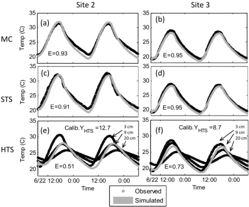
Fig. 3.Test 2 (Level 1) plots of temperature data for Site 2 and Site 3 in the main channel (MC)(a, b), STS(c, d), and HTS(e, f). Test 2 met the local criteria (E >0.8), but not the global criteria (AEs>0.7). Efor each location is shown in each subplot. The calibrated hyporheic
sediment depth (YHTSin cm) is shown in the HTS(e, f)with the observations at three depths labeled (3, 9 and 20 cm). The temperature data
sets closest to thisYHTSare used to calculate theEHTSsince observations at multiple depths were available.
Site 2 Site 3
MC
(b) (a)
(c) (d)
! STS
(c) (d)
Site 2
Site 3
MC
STS
(a)
(b)
(c)
(d)
HTS
(f)
(e)
!" # $ % #
3 cm 9 cm 20 cm
3 cm 9 cm 20 cm
Fig. 5.Test 7 (Level 2) plots of temperature data for Site 2 and Site 3 in the main channel (MC)(a, b), STS(c, d), and HTS(e, f). E, the performance at each location, is shown in each subplot. The calibrated hyporheic sediment depth (YHTSin cm) is shown in the HTS(e, f)
with the observations at three depths labeled (3, 9 and 20 cm).
4.2 Level 2
Level 2 simulations were used to determine which parame-ter sets resulting from the two-objective optimizations (Tests 5–10) converge to the established criteria ofE >0.8 for all calibration data sets and AEs>0.7 (Table 3). The E val-ues reported for the two-objective optimizations are based on the parameter set that represents the best trade-off solu-tion or the pareto solusolu-tion (Vrugt et al., 2003a,b; Boyle et al., 2000; Gupta et al., 1998, 2003; Neilson et al., 2010a). The best results are from Test 7 with values of7EMC2,Tr= 0.94, 7E
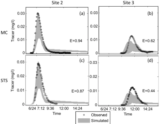
MC2,Temp= 0.91, and AEs= 0.81 (Table 3). Figures 5 and 6 present Test 7 results where the uncertainty bounds result-ing from pareto optimal parameter sets are shown. The un-certainty in the temperature predictions are less at Site 2 (Fig. 5) and there is a much better fit in terms of timing of the tracer curve at Site 2 (Fig. 6), compared to Level 1 re-sults, but there are still relatively large bounds. It should also be noted that this calibration does not capture the peak of the tracer at Site 3, nor the tail of the tracer curve at Site 2, which is critical to understanding the transient storage within the study reach (Bencala and Walters, 1983). Simi-lar to what Neilson et al. (2010a) found, comparing Level 1 and 2 results (Table 3) illustrates the relative benefit of us-ing two-objective optimization compared to sus-ingle-objective optimizations. For Tests 5–10, Tests 6 and 10 did not meet
the local criteria ofE >0.8 with tracer data used as a cali-bration objective, although Test 6 did meet the global criteria (Table 3).
Site 2 Site 3
MC
(b) (a)
(c) (d)
! " STS
(c) (d)
Fig. 6. Test 7 (Level 2) plots of tracer data with results at Site 2 and Site 3 in the main channel (MC)(a, b), and STS(c, d). E, the local performance at each location, is shown in each subplot.
ß1 Acs,STS1 αSTS1 QHTS1 YHTS1 Ygr ß2 Acs,STS2 αSTS2 QHTS2 YHTS2
Fig. 7.The parameter bounds for 11 calibrated parameters within the normalized a priori seach space [0, 1]. The parameter sets which met the global and local performance criteria for single objective and two-objective tests, Levels 1 and 2, are used to define a narrowed search space (the grey shaded area) for the Level 3 and 4 calibrations. The black lines represent the bounds of the Pareto optimal parameter sets from Level 1 and 2 calibrations.
4.3 Level 3 and Level 4
Similar to Level 1 results, Tests 1 through 4 all converged to E >0.9 for the data used in calibration during the Level 3 calibrations (Table 5). However, model performance at other locations was poor with the exception of Test 3, which had better AE results than Level 1: 3AEs= 0.76, and 3AEall= 0.62. While these results are promising, it is impor-tant to note that only the tracer at Site 2 (the calibration ob-jective) fit the observations well (not shown here for brevity). Level 4 had improved results when compared to Lev-els 1–3. The AEall and AEs values increased for most tests
Site 2
Site 3
MC
STS
(a)
(b)
(c)
(d)
HTS
(e)
(f)
!" # $ % # 3 cm
9 cm 20 cm
3 cm 9 cm 20 cm
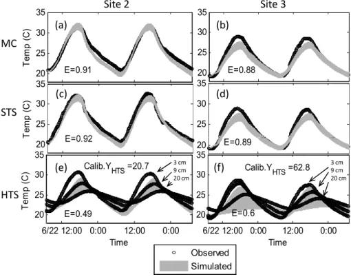
Fig. 8.Test 9 (Level 4) plots of temperature data for Site 2 and Site 3 in the main channel MC(a, b), STS(c, d), and HTS(e, f), where the observations at three depths are labeled (3, 9 and 20 cm).E, the performance at each location, is shown in each subplot.
Site 2
Site 3
MC
(b)
(a)
(c)
(d)
! "
STS
(c)
(d)
ß1 Acs,STS1 αSTS1 QHTS1 YHTS1 Ygr ß2 Acs,STS2 αSTS2 QHTS2 YHTS2 !
Fig. 10.The parameter sets which met the global and local performance criteria for multiple objective tests in Level 4, Test 9, are shown in grey within the bounds of all of the Pareto optimal parameter sets from Test 9 (black lines). The narrowed search space for the Level 3 and Level 4 calibrations, derived from the Level 1 and Level 2 results, is shown with the dashed line (shown as the grey area in Fig. 7). The a priori search space is the [0, 1] normalized bounds.
Table 3. Results for single objective (SO, Level 1) and multi-objective (MO, Level 2) calibration tests. Including HTS data gives the AEallresult shown in Column 1, excluding HTS and using only
main channel (MC) and STS data resulted in AEsshown in
Col-umn 2. Following the AEalland AEsresults are theEresults for
each test in the simulation matrix. Eand AEs were used to
de-termine the best models using parameter sets that meet both local (E >0.8) and global (AES>0.7, bolded) criteria. AEall was in-cluded for comparison to Level 3 and 4 calibrations. Shown in grey shading are the Site 2 and Site 3 locations in the main channel used for a calibration objective; unshaded boxes in Columns 3–6 are lo-cations where data were withheld during the calibration.
AEall AEs Site 2 Site 3 Site 2 Site 3 Temp Temp Tracer Tracer
MC MC MC MC
Level 1
1 – SO Temp 2 0.30 0.36 0.95 0.87 0.32 −0.10 2 – SO Temp 3 0.60 0.65 0.93 0.95 0.23 0.72 3 – SO Tr 2 0.34 0.50 0.72 0.91 0.96 −0.42 4 – SO Tr 3 0.16 0.42 0.89 0.92 −0.70 0.96
Level 2
5 – MO Temp 2 Temp 3 0.42 0.46 0.96 0.93 0.36 0.11 6 – MO Tr 2 Tr 3 0.61 0.76 0.83 0.93 0.35 0.99 7 – MO Temp 2 Tr 2 0.75 0.81 0.91 0.88 0.94 0.62 8 – MO Temp 3 Tr 2 0.39 0.57 0.86 0.94 0.98 −0.17 9 – MO Temp 2 Tr 3 0.47 0.58 0.91 0.93 −0.16 0.92 10 – MO Temp 3 Tr 3 0.65 0.68 0.91 0.95 0.94 0.12
provide the information necessary to achieve an acceptable global calibration.
Figure 10 shows the parameter ranges resulting from the Test 9 optimization that met the local and global criteria and the bounds of all the pareto optimal sets. The dashed line shows the narrowed parameter range within the original a priori search range (normalized here [0, 1]). The thick black line is the bounds of the pareto optimal parameter sets. The grey area is the parameter variability given the parameter sets
which meet both local and global performance criteria. This global fit resulted in a better representation of the dominant processes controlling instream processes, where the final re-duction of bounds in the upstream section was by an average of 49 % and the in the downstream section by an average of 69 %.
5 Discussion
Comparing the results of the simulation matrix calibrations when using only the main channel temperatures or tracer concentrations as an objective (Test 1–4, Table 3), we see how the choice of a calibration objective affects the global performance of the model by comparing the AEs and AEall values. In general, the best individual temperature and tracer main channel result is from a single objective optimization of that constituent at that location, but the corresponding model results are generally inappropriate at other locations. Our re-sults also show that when a main channel temperature objec-tive at one location results in reasonable predictions, the tem-perature at the other location will also be reasonable. How-ever, this is not necessarily the case when using tracer data in single objective optimizations in this study.
The best Level 2 local results at Site 2 and Site 3 for tracer are8EMC2,Tr= 0.98 and6EMC3,Tr= 0.99 and for temperature are5EMC2,Temp= 0.96 and 10EMC3,Temp= 0.95 (Table 3). It is interesting that the best fit for tracer at Site 3 uses tracer information at both Site 2 and 3 (Test 6), but the best fit at Site 2 uses tracer information at Site 2 and temperature infor-mation at Site 3 (Test 8). In this case, the tradeoff between solute at two sites is greater than the tradeoff between solute and temperature. For temperature, the best fit at Site 2 uses temperature data at both Site 2 and Site 3 (Test 5). However, the best temperature fit at Site 3 uses temperature and tracer data at Site 3 (Test 10). It should be noted that when tempera-ture data at Site 3 and tracer data at Site 2 were used (Test 8), 8E
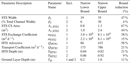
Table 4. The 11 calibration parameters distributed between two sites, the narrowed upper and lower parameter bounds, and associated percent reduction in parameter range compared to the a priori values shown in Table 2. The a priori range was the same for each section, but the narrowed bounds resulting from calibration varied between Sects. 1 and 2.
Parameter Description Parameter Sect. Narrow Narrow Bound
Name Lower Upper reduction
Bound Bound (%)
STS Width β1 1 19 35 47 %
(% Total Channel Width) β2 2 6 30 4 %
STS CS Area Ac,STS1 1 0.8 1.3 67 %
(m2) Ac,STS2 2 1.0 2.4 44 %
STS Exchange Coefficient αSTS1 1 3.8×10⁴ 8.1×10⁴ 38 %
(m2d−1) αSTS2 2 2.2×10⁴ 8.1×10⁴ 15 %
HTS Advective QHTS1 1 86 415 58 %
Transport Coefficient (m3d−1) QHTS2 2 173 786 21 %
HTS Depth (m) YHTS1 1 0.04 0.82 21 %
YHTS2 2 0.06 0.92 9 %
Ground Layer Depth (m) Ygr 1 and 2 0.2 1.0 11 %
tracer data at two different longitudinal locations provided more information about the system than just one data type.
While these local results give insight into the utility of calibration data, it is important to acknowledge how each of these calibrations perform globally. Given a broad pa-rameter search range (Level 2), Test 7 had the best over-all results with AEs= 0.81 and provided some corroboration of the model representing the dominant processes with an AEall= 0.75. Most Level 2 AEsand AEallvalues were higher than Level 1 values. This is consistent with the findings of Neilson et al. (2010a) who noted that two-objective tions performed better at locations not used in model calibra-tion than did single objective calibracalibra-tions. While Test 7 had the best global value, the individual results were not nearly as good as the best fits at each location for each data type. It did, however, provide the necessary information to narrow the search bounds for the Level 3 and 4 simulations.
With this initial understanding of the importance of sin-gle versus two-objective calibration and various data types in model calibration to narrow the search space, Level 3 and 4 results provide a more complete picture of how the system is functioning (Table 5). The majority of the Level 3 single-objective optimizations have AEs and AEall values that are higher than those in the Level 1 simulations. The actualE values for the location being used in the calibration are also higher with the exception of Test 1. This suggests that the more narrow search range was appropriate.
The best Level 4 results at Site 2 and Site 3 for tracer are8EMC2,Tr=6EMC2,Tr= 0.98 and10EMC3,Tr= 0.99 and for temperature are 7EMC2,Temp= 0.95 and 5EMC3,Temp = 10E
MC3,Temp= 0.94 (Table 5). The best tracer results at Site 2 are consistent with the Level 2 results where tracer informa-tion at Site 2 and temperature informainforma-tion at Site 3 is most appropriate (Test 8). The best Site 3 tracer results suggest
Table 5. Results for single objective (SO, Level 3, Tests 1–4) and multi-objective (MO, Level 4, Tests 5–10) calibration tests usingE
and AEsto determine the best model results using parameter sets
that meet both local (E >0.8) and global (AEs>0.7, bolded)
crite-ria. Including HTS data gives theAEallresult shown in Column 1.
Following the AEalland AEsresults are theEresults for each test
in the simulation matrix. Shown in grey shading are the Site 2 (S2) and Site 3 (S3) main channel (MC) information used as the temper-ature (Temp) and solute tracer (Tr) calibration objectives; unshaded boxes are locations where data were withheld during the calibration.
AEall AEs Site 2 Site 3 Site 2 Site 3
Temp Temp Tracer Tracer
MC MC MC MC
Level 3
1 – SO Temp S2 0.34 0.45 0.94 0.81 0.35 0.04 2 – SO Temp S3 0.64 0.7 0.91 0.95 0.81 0.33 3 – SO Tr S2 0.62 0.76 0.79 0.84 0.98 0.61 4 – SO Tr S3 0.64 0.69 0.92 0.94 0.06 0.99
Level 4
5 – MO Temp S2 Temp S3 0.73 0.76 0.94 0.94 0.59 0.71 6 – MO Tr S2 Tr S3 0.72 0.9 0.79 0.91 0.98 0.97 7 – MO Temp S2 Tr S2 0.41 0.48 0.95 0.83 0.53 −0.10 8 – MO Temp S3 Tr S2 0.66 0.79 0.79 0.83 0.98 0.72 9 – MO Temp S2 Tr S3 0.78 0.9 0.82 0.92 0.90 0.98 10 – MO Temp S3 Tr S3 0.67 0.75 0.89 0.94 0.26 0.99
that both temperature and tracer data at Site 3 (Test 10) is better than tracer data at Site 2 and Site 3 (Test 6). Within the narrow search bounds, the best tracer results rely on tem-perature information at some location.
Site 3 still uses temperature and tracer data at Site 3 (Test 10), but the results for Test 5 (which uses Site 2 and 3 tem-peratures) have the sameE. These results demonstrate the need to use both temperature and solute data in two-objective TZTS calibration. The Level 4 results also showed a marked improvement in most AEs and AEall values from Level 1– 3 simulations. This improvement can be related to the in-creased parameter certainty when comparing Level 2, Test 7 (Fig. 7) with Level 4, Test 9 (Fig. 10). These figures show the usefulness of using more information, or local data, to define a narrow range bounding the global optimum. They also highlight the importance of multi-objective calibrations to capture the spatial heterogeneity within streams and rivers and the need to determine the appropriate optimization pa-rameter ranges.
To further incorporate important physical processes and continue advancing our predictive capabilities, there is a need for a connected cycle of inquiry that includes model develop-ment and refinedevelop-ment, identification of data types and scales of measurement required to support modeling, and estab-lishing the most effective approach for calibration based on the application of interest. Since data collection methods to support parameter estimation in two zone transient storage modeling are evolving (e.g., Briggs et al. 2009; Neilson et al., 2010a,b), the need for flexibility when incorporating dynamic external information is underscored in model cali-bration particularly when dealing with both local and global scales. This type of flexibility is not available when opti-mization algorithms rely solely on the options encoded to solve the problem, which is the case for most single ob-jective algorithms (e.g., nonlinear gradient-based search al-gorithms such as the Levenberg-Marquardt algorithm (Mar-quardt, 1963, used by Hil, 1998; Doherty, 2005; Poeter et al., 2005), evolutionary algorithms (Duan et al., 1992; Deb, 2001) or Bayesian approaches (Metropolis et al., 1953; Hast-ings, 1970; Doherty, 2003). Although multi-objective algo-rithms (e.g., Gupta et al., 1998; Boyle et al., 2000; Madsen, 2000, 2003; Madsen et al., 2002; Deb et al., 2002; Vrugt et al., 2003a,b) and multi algorithm genetically adaptive search methods (AMALGAM, Vrugt and Robinson, 2007) incor-porate multiple datasets into optimization, the number of datasets considered have generally been limited to two or three time series and there is limited flexibility in the ob-jectives considered due to limitations of the algorithm design requirements (e.g., soil hydraulic models calibrated to mul-tiple soil depths, but only at one location; W¨ohliing et al., 2008).
The approach presented here builds on those of Vrugt (2003a), also used in W¨ohliing et al. (2008), where results from single objective optimizations are used to construct the boundaries of the search space. However, we use results from two-objective optimization studies to establish search space boundaries while considering multiple locations (MC and STS at two sites), multiple environmental tracers (tem-perature and solute), and using additional information for
corroboration (HTS temperatures). Rather than limiting the optimization search, we approach the problem from more angles by including all information available, iteratively ap-proaching optimal parameter sets, and highlighting the most important datasets for model calibration.
Consistent with what others have found (Gupta et al., 1998; Vrugt et al., 2003a; Neilson et al., 2010b), multi-objective optimization approaches were found to be more ef-fective and efficient at determining appropriate calibrations and data sets compared to single-objective optimizations. Additionally, multi-objective optimization results assisted in assessing the utility of datasets in narrowing the parameter bounds due to consideration of tradeoffs between objectives. We found that inclusion of all available site specific data in model calibration and corroboration not only provided in-formation that decreased the number and range of param-eters, but also provided information about model certainty, can guide the incorporation of processes missing in the con-ceptual model in future model development work, and will assist in prioritization of future data collection efforts.
6 Conclusions
With the overall goal of iteratively reducing the size of the global search space while simultaneously investigating the information content within the available data types, we es-tablished a simulation matrix to test the use of the most com-monly collected main channel data sets used for model cal-ibration of instream temperature and solute models. This systematic approach to using multiple types of distributed information allowed us to examine the application of both single and multi-objective optimization algorithms to the TZTS model using both temperature and solute data avail-able within the main channel and transient storage zones (STS and HTS). In the context of a case study in the Vir-gin River, Utah, USA, our global problem was to optimize the model given ten time series distributed in space. Our lo-cal problem was that any unacceptable parameter set (i.e., the model does not represent one observed time series well) signified a failure to adequately reproduce the dominant pro-cesses affecting both the heat and solute response at that lo-cation.
and in the downstream section by an average of 17 %. Level 3 and 4 calibrations, based on narrowed parameter bounds, led to improved predictions of instream temperatures and tracer concentrations at multiple locations and zones in the study area not used in calibration. This global fit resulted in a bet-ter representation of the dominant processes controlling in-stream processes, where the final reduction of bounds in the upstream section was by an average of 49 % and in the down-stream section by an average of 69 %.
Another key finding was that, in general, using both main channel temperature and solute data in calibration provided better global results. Therefore, we suggest that both data types be collected at different locations, for example, solute at one calibration site and temperature at another. Based on the results of this study, and the need to use resources associ-ated with data collection more efficiently, we recommend fu-ture data collection focused on collecting a single tracer ob-servation time series in the main channel, with temperatures collected simultaneously in multiple locations and zones to be used in model calibration and testing.
Acknowledgements. We are indebted to those who helped collect the data that supported this paper (Quin Bingham, Noah Schmadel, Jon Bingham, Andrew Hobson, Ian Gowing, Bayani Cardenas, Enrique Rosero, and Lindsey Goulden). We would also like to thank the USGS and Washington County Water Conservancy District for providing funding and/or support for multiple data collection efforts within the Virgin River. Additional thanks to the anonymous reviewers that provided thoughtful reviews of the manuscript.
Edited by: M. Gooseff
References
Ajami, N. K., Duan, Q., and Sorooshian, S.: An Integrated Hy-drologic Bayesian Multi-Model Combination Framework: Con-fronting Input, Parameter and Model Structural Uncertainty in Hydrologic Prediction, Water Resour. Res., 43, W01403, doi:10.1029/2005WR004745, 2007.
Bencala, K. E. and Walters, R. A.: Simulation of solute transport in a mountain pool-and-riffle stream: a transient storage model, Water Resour. Res., 19, 718–724, 1983.
Beven, K.: Rainfall-Runoff Modelling: The Primer, John Wi-ley & Sons, LTD, Chichester, England, 2001.
Bingham, Q. G.: Data Collection and Analysis Methods for Two-Zone Temperature and Solute Model Parameter Estimation and Corroboration, http://digitalcommons.usu.edu/etd/564, last ac-cess: 10 May 2011, M. S. Thesis, Utah State University, Logan, USA, 2010.
Blasone, R.-S., Vrugt, J. A., Madsen, H., Rosbjerg, D., Robinson, B. A., and Zyvoloski, G. A.: Generalized likelihood uncertainty estimation (GLUE) using adaptive Markov Chain Monte Carlo sampling, Adv. Water. Resour., 31, 630–648, 2008.
Boyle, D. P., Gupta, H. V., and Sorooshian, S.: Toward Improved Calibration of Hydrologic Models: Combining the Strengths of Manual and Automatic Methods, Water Resour. Res., 36, 3663– 3674, 2000.
Briggs, M. A., Gooseff, M. N., Arp, C. D., and Baker, M. A.: A Method for Estimating Surface Transient Storage Parameters for Streams with Concurrent Hyporheic Exchange, Water Resour. Res., 45, W00D27, doi:10.1029/2008WR006959, 2009. Deb, K.: Multi-objective optimization using evolutionary
algo-rithms. John Wiley & Sons, Chichester, UK, 2001.
Deb, K., Pratap, A., Agarwal, S., and Meyarivan, T.: A fast and elitist multiobjective genetic algorithm: NSGA-II, IEEE Trans. Evolut. Comput., 6, 182–197, 2002.
Doherty, J: MICA: Model-Independent Markov Chain Monte Carlo Analysis, Watermark Numerical Computing, Brisbane, Aus-tralia, 2003.
Doherty, J.: PEST: Software for Model-Independent Parameter Es-timation. Watermark Numerical Computing, Australia, available from: http://www.sspa.com/pest (last access: 10 May 2011), 2005.
Duan, Q. S., Sorooshian, S., and Gupta, V. K.: Effective and effi-cient global optimization for conceptual rainfall runoff models, Water Resour. Res., 28(4), 1015–1031, 1992.
Duan, Q.: Global Optimization for Watershed Model Calibration, in: Calibration of Watershed Models, edited by: Duan, Q., Gupta, H. V., Sorooshian, S., Rousseau, A. N., and Turcotte, R., American Geophysical Union, Washington, DC, 2003.
Duan, Q., Ajami, N. K., Gao, X., and Sorooshian, S.: Multi-Model Ensemble Hydrologic Prediction Using Bayesian Model Averag-ing, Adv. Water Resour., 30, 1371–1386, 2007.
Everts, C. J. and Kanwar, R. S.: Evaluation of Rhodamine WT as an absorbed tracer in an agricultural soil, J. Hydrol., 153, 53–70, 1994.
Fu, J. and G´omez-Hern´andez, J.: Uncertainty assessment and data worth in groundwater flow and mass transport modeling using a blocking Markov chain Monte Carlo method, J. Hydrol., 364, 328–341, 2009.
Gupta, H. V., Sorooshian, S., and Yapo, P. O.: Toward Improved Calibration of Hydrologic Models: Multiple and Noncommensu-rable Measures of Information, Water Resour. Res., 34, 751–776, 1998.
Gupta, H. V., Bastidas, L. A., Vrugt, J. A., and Sorooshian, S.: Mul-tiple Criteria Global Optimization for Watershed Model Calibra-tion, in: Calibration of Watershed Models, edited by: Duan, Q., Gupta, H. V., Sorooshian, S., Rousseau, A. N., and Turcotte, R., American Geophysical Union, Washington, DC, 2003.
Hastings, W. K.: Monte Carlo sampling methods using Markov chains and their applications, Biometrika, 57, 97–109, 1970. Herbert, L. R.: Seepage Study of the Virgin River from Ash Creek
to Harrisburg Dome, Washington County, Utah, Rep. Technical Publication no. 106, United States Geological Survey/State of Utah Department of Natural Resources, 1995.
Hill, M. C.: Methods and Guidelines for Effective Model Calibra-tion, US Geological Survey Water-Resources Investigations Re-port 98-4005, 1998.
Madsen, H.: Automatic calibration of a conceptual rainfall-runoff model using multiple objectives, J. Hydrol., 235, 267–288, 2000. Madsen, H.: Parameter estimation in distributed hydrological catch-ment modelling using automatic calibration with multiple objec-tives, Adv. Water Resour., 26, 205–216, 2003.
Madsen, H., Wilson, G., and Ammentorp, H. C.: Comparison of different automated strategies for calibration of rainfall-runoff models, J. Hydrol., 261, 48–59, 2002.
Marquardt, D. W.: An algorithm for least-squares estimation of nonlinear parameters, J. Soc. Ind. Appl. Math., 11, 431–441, 1963.
Metropolis, N., Rosenbluth, A. W., Rosenbluth, M. N., Teller, A. H., and Teller, E.: Equations of state calculations by fast computing machines, J. Chem. Phys., 21, 1087–1091, 1953.
Nash, J. E. and Sutcliffe, J. V.: River Flow Forecasting through Conceptual Models Part 1 – a Discussion of Principles, J. Hy-drol., 10, 282–290, 1970.
Neilson, B. T., Chapra, S. C., Stevens, D. K., and Bandaragoda, C. J.: Two-zone transient storage modeling using temperature and solute data with multi-objective calibration: Part 1 Temperature, Water Resour. Res., 46, W12520, doi:10.1029/2009WR008756, 2010a.
Neilson, B. T., Stevens, D. K., Chapra, S. C., and Bandaragoda, C. J.: Two-zone transient storage modeling using tempera-ture and solute data with multi-objective calibration: Part 2 Temperature and Solute, Water Resour. Res., 46, W12521, doi:10.1029/2009WR008759, 2010b.
Poeter, E. P., Hill, M. C., Banta, E. R., Mehl, S., and Christensen, S.: UCODE 2005 and Six Other Computer Codes for Universal Sen-sitivity Analysis, Calibration, and Uncertainty Evaluation, avail-able from: http://www.mines.edu/igwmc/freeware/ucode/ (last access: 10 May 2011), 2005.
Schaake, J.: Introduction, in: Calibration of Watershed Models, edited by: Duan, Q., Gupta, H. V., Sorooshian, S., Rousseau, A. N., and Turcotte, R., American Geophysical Union, Washington, DC, 2003.
Shiau, B.-J., Sabatini, D. A., and Harwell, J. H.: Influence of rho-damine WT properties on sorption and transport in subsurface media, Ground Water, 31, 913–920, 1993.
Vrugt, J. A. and Robinson, B. A.: Treatment of uncertainty using ensemble methods: Comparison of sequential data assimilation and Bayesian model averaging, Water Resour. Res., 43, W01411, doi:10.1029/2005WR004838, 2007.
Vrugt, J. A., Gupta, H. V., Bastidas, L. A., Bouten, W., and Sorooshian, S.: Effective and Efficient Algorithm for Multiob-jective Optimization of Hydrologic Models, Water Resour. Res., 39, 1214, doi:10.1029/2002WR001746, 2003a.
Vrugt, J. A., Gupta, H. V., Bouten, W., and Sorooshian, S.: A Shuf-fled Complex Evolution Metropolis Algorithm for Optimization and Uncertainty Assessment of Hydrologic Model Parameters, Water Resour. Res., 39, 1201, 2003b.
Wagener, T., Boyle, D. P., Lees, M. J., Wheater, H. S., Gupta, H. V., and Sorooshian, S.: A framework for development and applica-tion of hydrological models, Hydrol. Earth Syst. Sci., 5, 13–26, doi:10.5194/hess-5-13-2001, 2001.