Predictability, stationarity, and classification of hydraulic responses to recharge in two karst aquifers

(1)

HESSD

9, 9577–9609, 2012

Hydraulic responses to recharge in two

karst aquifers

A. J. Long and B. J. Mahler

Title Page

Abstract Introduction

Conclusions References

Tables Figures

◭ ◮

Back Close

Full Screen / Esc

Printer-friendly Version Interactive Discussion

Discussion

P

a

per

|

Dis

cussion

P

a

per

|

Discussion

P

a

per

|

Discussio

n

P

a

per

|

Hydrol. Earth Syst. Sci. Discuss., 9, 9577–9609, 2012 www.hydrol-earth-syst-sci-discuss.net/9/9577/2012/ doi:10.5194/hessd-9-9577-2012

Hydrology and Earth System Sciences Discussions

This discussion paper is/has been under review for the journal Hydrology and Earth System Sciences (HESS). Please refer to the corresponding final paper in HESS if available.

Predictability, stationarity, and

classification of hydraulic responses to

recharge in two karst aquifers

A. J. Long1and B. J. Mahler2

1

US Geological Survey, 1608 Mountain View Rd, Rapid City, South Dakota, 57702, USA

2

US Geological Survey, 505 Ferguson Lane, Austin, Texas, 78754, USA

Received: 7 August 2012 – Accepted: 8 August 2012 – Published: 16 August 2012

Correspondence to: A. J. Long (ajlong@usgs.gov)

(2)

HESSD

9, 9577–9609, 2012

karst aquifers

Title Page

Tables Figures

◭ ◮

Back Close

Full Screen / Esc

Discussion

P

a

per

|

Dis

cussion

P

a

per

|

Discussion

P

a

per

|

Discussio

n

P

a

per

|

Abstract

Karst aquifers, many of which are rapidly filled and depleted, are likely to be highly susceptible to changes in short-term climate variability. Here we explore methods that could be applied to model site-specific hydraulic responses, with the intent of simulat-ing these responses to different climate scenarios from high-resolution climate models.

5

We compare hydraulic responses (spring flow, groundwater level, and stream base flow) at several sites in two karst aquifers: the Edwards aquifer (Texas, USA) and the Madison aquifer (South Dakota, USA). A one-dimensional, lumped-parameter model simulates nonstationary soil moisture changes for estimation of recharge, and a non-stationary convolution model simulates the aquifer response to this recharge. Model fit

10

to data was 4 % better for calibration periods than for validation periods. We use met-rics that describe the shapes of the impulse-response functions (IRFs) obtained from convolution modeling to make comparisons in the distribution of response times among sites and among aquifers. Combined principal component analysis and cluster analysis of metrics describing the shapes of the IRFs separated those sites with IRFs having

15

a large ratio of the mean response time to the system memory from those with large skewness and kurtosis. Classification of the IRF metrics indicate that there is a range of IRF characteristics for different site types (i.e., spring flow, groundwater level, base flow) within a karst system. Further, similar site types did not necessarily display similar IRFs. Results indicate that the di_fferences existing within either aquifer are larger than

20

the differences between the two aquifers and that the two aquifers are similar according to this classification. The use of multiple metrics to describe the IRFs provides a novel way to characterize and compare the way in which multiple sites respond to recharge. As convolution models are developed for additional aquifers, they could contribute to an IRF database and a general classification system for karst aquifers.

(3)

HESSD

9, 9577–9609, 2012

karst aquifers

Title Page

Tables Figures

◭ ◮

Back Close

Full Screen / Esc

Discussion

P

a

per

|

Dis

cussion

P

a

per

|

Discussion

P

a

per

|

Discussio

n

P

a

per

|

1 Introduction

An understanding of how key hydrologic variables, such as spring flow and groundter levels, are likely to respond to potential future climate scenarios is critical for wa-ter management. Karst aquifers are likely to be particularly susceptible to changes in short-term climate variability because the cavernous porosity of these aquifers allows

5

rapid replenishment by focused recharge through streambeds and sinkholes (White, 1988), the amount and timing of which is tightly linked to precipitation and antecedent moisture conditions (e.g., Long, 2009; Jukić and Denić-Jukić, 2011). The karstic Ed-wards Balcones Fault Zone aquifer has been identified as being particularly vulnerable to climate-change effects because of high use, strong links to climatic inputs, large

10

variability in precipitation and multi-year droughts, and dependent endangered species (Lo ´aiciga et al., 2000).

High-resolution weather-forecast models have been adapted to simulate regional climate change based on boundary conditions taken from coarser-resolution general circulation models (e.g., Mearns et al., 2009; Hostetler et al., 2011). With regional

cli-15

mate models continually improving, convolution modeling is a promising approach to estimate how hydrologic systems will respond to local-scale climate scenarios. Convo-lution has been widely used in rainfall-runoffmodels to simulate streamflow in response to infiltration on a watershed (Singh, 1988; Jakeman and Hornberger, 1993; Jeannin, 2001; Pinault et al., 2001; Simoni et al., 2011). Convolution also has been applied, to

20

a lesser extent, to groundwater response (Hall and Moench, 1972; Long and Derick-son, 1999; Jukić and Denić-Jukić, 2006). Convolution is particularly useful for simu-lating karst hydrologic systems, which respond rapidly to changes in precipitation but for which site-specific response is difficult if not impossible to simulate with physically based numerical models. Unsteady and nonuniform flow in variably saturated conduits

25

(4)

HESSD

9, 9577–9609, 2012

karst aquifers

Title Page

Tables Figures

◭ ◮

Back Close

Full Screen / Esc

Discussion

P

a

per

|

Dis

cussion

P

a

per

|

Discussion

P

a

per

|

Discussio

n

P

a

per

|

types of karst aquifers (e.g., Smart and Worthington, 2004), but only a few of the pro-posed approaches are quantitative, as in Covington et al. (2009, 2012) and Labat et al. (2011). Convolution modeling is well suited to quantification of characteristic aquifer metrics that describe hydraulic response types.

Here we explore methods that could be applied to model site-specific hydraulic

5

responses with the intent of application to projected climate simulations from high-resolution dynamical models, as these models continually improve. We compare hy-draulic response characteristics at several sites in two karst aquifers: the Edwards aquifer (Texas, USA) and the Madison aquifer (South Dakota, USA). We describe the application of a one-dimensional, lumped-parameter model on a site-specific basis

10

and quantification of the predictive accuracy of model output. We examine and quan-tify temporal nonstationarity, a condition common in karst systems especially when epiphreatic conduits exist (Jeannin, 2001). The model simulates nonstationary soil moisture changes for estimation of recharge and uses a nonstationary convolution pro-cess to simulate the aquifer response to this recharge. We used metrics that describe

15

the shapes of the IRFs obtained from convolution modeling to make comparisons be-tween sites and bebe-tween two aquifers in a novel approach that could be useful for karst aquifer classification.

2 Methods

2.1 Estimating recharge

20

(5)

HESSD

9, 9577–9609, 2012

karst aquifers

Title Page

Tables Figures

◭ ◮

Back Close

Full Screen / Esc

Discussion

P

a

per

|

Dis

cussion

P

a

per

|

Discussion

P

a

per

|

Discussio

n

P

a

per

|

s_i =cr_i+1₋κ−1

i

s_i₋1 (1)

=c

r_i+1₋κ−1

i

s_i₋1+

1₋κ−1

i

2

s_i₋2+. . .

i =0, 1,. . .,N 0> s >1, (2)

wherec is a normalizing parameter that limits s to values between 0 and 1 (dimen-sionless),κ adjusts the influence of antecedent conditions and is related to

evapotran-5

spiration (dimensionless),r is total daily rainfall (cm), and i is the time step (days). Air temperature, which influences evapotranspiration rates, is accounted for by adjusting κby daily air temperature (Jakeman and Hornberger, 1993):

κi =αexp [(20−Ti)f] f >0, (3)

whereαis scaling coefficient (dimensionless),T is air temperature (◦_{C), and}_f _{is a}

tem-10

perature modulation factor (◦_C−1_{). Equation (3) has the primary e}_ff_{ect of increasing the} value of s during cool periods (0< T <20◦_{C) when evapotranspiration is low. Daily} recharge, or effective precipitation,ui (cm) is then calculated by

u_i =r_is_i. (4)

Only precipitation that occurs either as rain or melting snow was included in calculation

15

ofs. A method was established to estimate the occurrence of snow precipitation and melting for future periods on the basis of simulated air temperature. To determine the form of precipitation for each day, an air temperature threshold value (Ts=0) was set, below which precipitation was assumed to occur as snow. To determine days when melting occurs, a melting threshold valueT_m was estimated. If daily snow-depth data

20

(6)

HESSD

9, 9577–9609, 2012

karst aquifers

Title Page

Tables Figures

◭ ◮

Back Close

Full Screen / Esc

Discussion

P

a

per

|

Dis

cussion

P

a

per

|

Discussion

P

a

per

|

Discussio

n

P

a

per

|

was multiplied bySf and summed for the continuous series of snow-precipitation days prior to each snowmelt day. This sum was added to each snowmelt day in the daily rainfall record because snowmelt was assumed to have the same effect as rainfall on the value ofs.

2.2 Convolution

5

If a system input, after being transported through a medium, results in a system output that is dispersed in time according to a characteristic waveform, then this system can be simulated by convolution. In karst settings, hydrologic responses that are suitable for simulation by convolution are hydraulic head (e.g., water level in a well) and flow (e.g., from a spring), which were simulated on a daily time step.

10

Convolution is described by

y(t)₌ ∞

Z

0

h(t₋τ)u(τ)dτ, (5)

wherey(t) is the system response function;u(τ) is the system input, or forcing function; h(t−τ) is an impulse-response function (IRF); andt andτ are time variables, where t₋τrepresents the delay time from signal to response (Singh, 1988; Olsthoorn, 2008).

15

For uniform time steps, the discrete form of Eq. (5) is

yi = i

X

j=0

hi₋juj i=0, 1,. . .,N. (6)

The IRF describes the system response functiony that results from an instantaneous unit input u_j. The length of the IRF quantifies the system memory, or time that the response to the impulse persists. IRFs were approximated by exponential or lognormal

20

curves or a combination of the two. The exponential curve is defined as

(7)

HESSD

9, 9577–9609, 2012

karst aquifers

Title Page

Tables Figures

◭ ◮

Back Close

Full Screen / Esc

Discussion

P

a

per

|

Dis

cussion

P

a

per

|

Discussion

P

a

per

|

Discussio

n

P

a

per

|

whereais a scaling coefficient, andλdetermines the mean and variance of the system response timetas

µ=λ−1 ₍₈₎

and

σ2=λ−4_, ₍₉₎

5

respectively. The lognormal curve is defined as

h(t)= b

t√2πεexp

−₂1_ε(lnt−ω)2

, (10)

wherebis a scaling coefficient, andωandεdetermine the mean and variance oftas

µ=exp ω+ε/2

(11)

and

10

σ2=µ2[exp(ε)₋1] , (12)

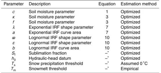
respectively. Parameters of Eqs. (1)–(12) are listed in Table 1. Because exponential and lognormal curves are asymptotic and thus have infinite length with infinitesimal magnitude after some point in time, system memory is defined herein as timet_m on the IRF time scale at which 95 % of the area of the curve is between timet=0 andtm.

15

Modeling of flow in karst settings is complicated by the existence of quick-flow and slow-flow components; e.g., flow through large conduits as well as small fractures (Pinault et al., 2001). In some cases, a single exponential or lognormal IRF can ade-quately represent the quick-flow and slow-flow components of karst groundwater flow, where the first part of the curve, including the initial peak, represents quick flow, and the

20

(8)

HESSD

9, 9577–9609, 2012

karst aquifers

Title Page

Tables Figures

◭ ◮

Back Close

Full Screen / Esc

Discussion

P

a

per

|

Dis

cussion

P

a

per

|

Discussion

P

a

per

|

Discussio

n

P

a

per

|

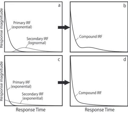
that represents all or part of the slow-flow component may be useful (e.g., Long, 2009). The resulting compound IRF is the superposition of the primary and secondary IRFs. Several authors have used compound IRFs to represent the quick-flow and slow-flow components in karst settings (e.g., Jakeman et al., 1993; Pinault et al., 2001; Denić-Jukić and Denić-Jukić, 2003). In the approach herein, the compound IRF can consist of any

5

combination of two IRFs, either exponential or lognormal (Fig. 1). A compound IRF con-sisting of an exponential and lognormal curve can result in a bimodal, or double-peak, distribution of response times, which could be a result of two-domain flow (Fig. 1b, Long and Putman, 2006). A compound IRF consisting of two exponential curves is useful when quick flow and slow flow are separated into a sharp initial peak and long

10

tail, respectively (Fig. 1d).

If the scaling coefficientsaandbare set to unity, the areas under the IRFs also are equal to unity. Adjusting the values of these coefficients allows their use as conver-sion factors to account for the di_fferent dimensions between the forcing function and response function and also allows for unequal response magnitudes between the

pri-15

mary and secondary IRFs. For simulation of groundwater levels, a datumh0 at which hydraulic head equals zero must be established. Conceptually, this is the level to which hydraulic head would converge if the local system-input recharge was eliminated. This system input is assumed to be the only source of recharge close enough to cause hydraulic-head fluctuation and the only source that causes hydraulic head to rise above

20

h0.

2.3 Nonstationarity

Antecedent soil moisture effects and complex geological and morphological structures result in nonstationarity in watershed flow processes (Simoni et al., 2011), which are those whose parameters change when shifted in time. For application to karst

water-25

(9)

HESSD

9, 9577–9609, 2012

karst aquifers

Title Page

Tables Figures

◭ ◮

Back Close

Full Screen / Esc

Discussion

P

a

per

|

Dis

cussion

P

a

per

|

Discussion

P

a

per

|

Discussio

n

P

a

per

|

In this model, nonstationary response characteristics are simulated at two different stages in the overall process. The first stage is the infiltration of precipitation to become recharge. Recharge rate is determined bys (Eqs. 1–4), which varies on a daily time scale resulting in nonstationarity at this stage. The second stage is the transformation of recharge to a hydraulic response, which is simulated by convolution (Eqs. 5–12).

5

The system response characteristics as described by the IRF are affected by changes in precipitation rates on a scale of years to decades. It therefore was useful to sepa-rate the precipitation record into wet and dry periods of 1 yr or greater, as determined on the basis of the annual cumulative departure from the long-term mean precipitation (CDMP). Periods with positive slopes in the CDMP occur when precipitation is

con-10

sistently above the mean and thus indicate wet periods; negative slopes indicate dry periods. To account for nonstationarity at the second stage, the shape parameters and scaling coefficients of the IRFs were estimated separately for wet and dry periods, with the assumption that the curve types do not change temporally within these periods. This is a method not previously used and has advantages for aquifer classification

be-15

cause wet-period and dry-period metrics are distinct and clearly defined. As many as four IRFs were used to simulate the system response during model calibration: primary IRFs (IRFw1and IRFd1) and secondary IRFs (IRFw2and IRFd2), where the subscripts, w and d, refer to wet and dry periods, respectively.

The IRF curve areas can be different for wet and dry periods and primarily are

mean-20

ingful in their relative magnitudes for comparison of the responses of these two periods, which may provide insight into system operation. For example, if a wet-period IRF has twice the area of a dry-period IRF, then the wet-period response is twice that of the dry period for the same amount of recharge.

2.4 Classification of site responses

25

(10)

HESSD

9, 9577–9609, 2012

karst aquifers

Title Page

Tables Figures

◭ ◮

Back Close

Full Screen / Esc

Discussion

P

a

per

|

Dis

cussion

P

a

per

|

Discussion

P

a

per

|

Discussio

n

P

a

per

|

comparisons can be made among the aquifers. The IRF is suitable for comparison of sites and aquifers in climatically di_fferent locations because this comparison does not depend on differences in rainfall frequency, variability, or intensity between locations.

We used metrics, which can be quantified for any parametric or nonparametric IRF, to quantify several characteristics of the IRF shapes (Table 2). Metrics were selected

5

that quantify the IRF shape independently from scale so that comparisons were not weighted by the overall IRF magnitude, which might vary for climatically different lo-cations. To define these metrics, the IRF was assumed to be a frequency distribution of the transit times of the response quantity, either hydraulic head or flow, and basic statistics and other parameters of this distribution were computed. Ratios were used for

10

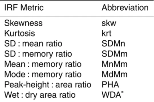
many of the metrics because these are scale independent. Metrics include skewness (skw), kurtosis (krt), and five ratios: standard-deviation : mean (SDMn), mean : memory (MnMm), mode : memory (MdMm), standard-deviation : memory (SDMm), and peak-height : area (PHA; for bimodal distributions the highest peak is used). These seven metrics were quantified for wet and dry periods separately (Table 2), resulting in 14

15

metrics. For stationary systems, wet and dry metrics are equal. Finally, the wet : dry area ratio (WDA) was included, which is the ratio of the wet-period to dry-period IRF area (WDA=1 for stationary systems) and results in a total of 15 metrics (Table 2).

Principal component analysis (PCA) and cluster analysis were used to assess simi-larities, differences, and groupings of sites on the basis of IRF shape, as described by

20

the 15 metrics. PCA is a linear transformation of data in multidimensional space, where the transformed axes, or principal components, align with the greatest variances in the multivariate dataset (Davis, 2002). Each principal component is a new variable that is a linear combination of all the original variables. PCA is helpful for elucidating patterns that would otherwise be obscured in attempting to assess a large number of metrics.

25

(11)

HESSD

9, 9577–9609, 2012

karst aquifers

Title Page

Tables Figures

◭ ◮

Back Close

Full Screen / Esc

Discussion

P

a

per

|

Dis

cussion

P

a

per

|

Discussion

P

a

per

|

Discussio

n

P

a

per

|

2.5 Modeling considerations

Convolution models provide a convenient way to assess system memory, which is an important consideration in any hydrologic model. At a minimum, input corresponding to a time period equal to the system memory is required prior to the start of a calibration period. This initial time period is referred to as model spin-up, the output from which is

5

considered to be of questionable validity.

The length of the calibration and validation periods also must be considered in light of the system memory. There is less confidence in the predictive strength of a model if the observed record is shorter than the system memory than if it is longer. Ideally, the validation period alone should be longer than the system memory, and if it is several

10

times longer than the system memory, the full range of response times is tested several times over.

The use of secondary IRFs, the choice of curve type, and stationarity were eval-uated and selected for each site on the basis of model fit for the validation period. Inclusion of secondary IRFs and simulating a system as nonstationary increase model

15

parameterization and complexity over the simpler options. In some cases the simplest model resulted in a better fit for the validation period than one with added complexity. Although model fit might improve for the calibration period as parameters are added, if the validation period indicates that this added complexity is not helpful, the model is overparameterized. If the overall model fit is poor, this model might not be appropriate,

20

or the input data might not represent the recharge area well.

3 Model application and results

Hydraulic responses at several sites with data for spring flow, groundwater base flow in streams, groundwater level, or cave drip (Table 3) were simulated for two karst aquifers: the Edwards aquifer in south-central Texas and the Madison aquifer in

west-25

(12)

HESSD

9, 9577–9609, 2012

karst aquifers

Title Page

Tables Figures

◭ ◮

Back Close

Full Screen / Esc

Discussion

P

a

per

|

Dis

cussion

P

a

per

|

Discussion

P

a

per

|

Discussio

n

P

a

per

|

were obtained from the National Climatic Data Center (2012). Generally, the recharge areas for the sites simulated are small, and data from a single weather station was used as model input. The weather station either within or nearest the recharge area for each site was used, and the next nearest station was used to fill periods of missing data if necessary. Equations (1), (3), (4), (6), (7), and (10) were programmed in

MAT-5

LAB (http://www.mathworks.com). The models were calibrated to observed discharge and water levels at gages (Table 3; US Geological Survey, 2012). Model parameters (Table 1) were optimized by using the “lsqcurvefit” function in MATLAB to minimize the differences (residuals) between simulated and observed temperature values. This is a subspace trust-region method and is based on the interior-reflective Newton method

10

(Coleman and Li, 1994, 1996).

3.1 Study areas

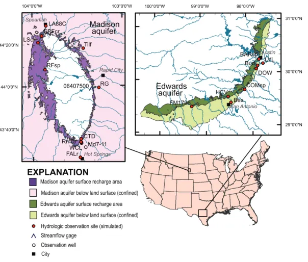
The Edwards Balcones Fault Zone aquifer (herein, the Edwards aquifer) in South-Central Texas is a well-developed karst aquifer contained within the Edwards Group. Surface recharge to the Edwards aquifer occurs from direct precipitation and sinking

15

streams that cross onto the outcrop area of the Edwards Group from the west and northwest (Fig. 2). The aquifer dips to the south and southeast below the land surface. Groundwater flow generally is to the east and northeast, and discharge occurs at sev-eral large springs. The hydrogeology of the Edwards aquifer is described in detail in Maclay and Small (1983), Small et al. (1996), and Lindgren et al. (2004).

20

The Madison aquifer in Western South Dakota is a well-developed karst aquifer com-posed of limestone and dolostone (Greene and Rahn, 1995). It is contained within the regionally extensive Madison Limestone of Mississippian age, referred to locally as the Pahasapa Limestone. This formation is exposed at the land surface on all flanks of the Black Hills and dips radially outward in all directions below the land surface (Fig. 2);

25

(13)

HESSD

9, 9577–9609, 2012

karst aquifers

Title Page

Tables Figures

◭ ◮

Back Close

Full Screen / Esc

Discussion

P

a

per

|

Dis

cussion

P

a

per

|

Discussion

P

a

per

|

Discussio

n

P

a

per

|

3.2 Sites simulated

For the Edwards aquifer, water level in six wells and flow from two large springs were simulated (Fig. 2, Table 3). For the Madison aquifer, three wells, one spring, one spring complex, one cave water body, and stream base flow for two Madison Limestone water-sheds were simulated (Fig. 2, Table 3). In addition, cave-drip at two sites and

stream-5

flow in one fractured-rock watershed located in the Madison study area were simulated for comparison to the aquifer sites (Fig. 2, Table 3). The observed and simulated spring flow for Barton Springs is shown as an example of simulation results (Fig. 3).

Daily precipitation and air temperature were used as model input for all sites, ex-cept for the Reptile Gardens well (site RG; Fig. 2, Table 3). This site is located in an

10

area where the primary recharge source is sinking streamflow, which was estimated as described in Hortness and Driscoll (1998) on a daily time step for streamflow gage 06407500 (Fig. 2) and used as model input.

Hydrologic response data for all of the Edwards aquifer sites consisted of direct water-level or spring-flow measurements, but additional description or data

manipula-15

tion was required for some of the Madison aquifer sites, e.g., because of indirect spring-flow measurements. Observed streamspring-flow at Little Spearfish Creek and Spearfish Creek (sites LScr and SPFcr) was used as an estimate of groundwater discharge, which is 97 % and 86 %, respectively, of total streamflow (Driscoll and Carter, 2001). Overland runoffin these watersheds rarely occurs because of the highly porous karst

20

terrain (Miller and Driscoll, 1998). Groundwater input to streamflow in the Fall River (site FALr) is about 96 %, primarily flowing from a complex of artesian springs (Rahn and Gries, 1973; Back et al., 1983; Driscoll and Carter, 2001). A 1-yr moving average of streamflow was used as a surrogate for total observed spring flow to remove an-thropogenic variability resulting from municipal water use and wastewater discharge.

25

(14)

HESSD

9, 9577–9609, 2012

karst aquifers

Title Page

Tables Figures

◭ ◮

Back Close

Full Screen / Esc

Discussion

P

a

per

|

Dis

cussion

P

a

per

|

Discussion

P

a

per

|

Discussio

n

P

a

per

|

streamflow at a daily time step was used as model input for the period prior to 1991 because data were not available for that period.

3.3 Calibration and validation of models

The models were validated by (1) calibrating each model to part of the record for the system response, (2) executing the model under those conditions for the remaining

pe-5

riod (validation period), and (3) examining the similarity of the simulated and observed system responses for the validation period. Calibration periods ranged from 0.9 to 70 yr and validation periods ranged from 0 to 23.8 yr (Table 4). Model parameters were ad-justed by trial and error until the simulated hydrographs were similar to the observed hydrographs. Parameter optimization then was executed for the calibration periods, and

10

the validation periods were evaluated on the basis of the Nash criterion (Nash and Sut-cli_ffe, 1970), which is a measure of the fit between simulated and observed time-series records, hereafter referred to asmodel fit. The Nash criterion is defined as

CNash=1−

P

(yobs−ysim) 2

P

(yobs−ymean)

2, (13)

whereyobs and ysim are daily time-series of the observed and simulated responses,

15

respectively, andymean is the mean ofyobs. The Nash criterion varies from 0 (poorest fit) to 1.0 (best fit) and is a comparison of the magnitude of residuals (numerator) to the overall amplitude of fluctuation in the observed record (denominator).

The Nash criterion was calculated for the calibration and validation periods sepa-rately (C_Nash-cand C_Nash-v; Table 4). For comparison of residuals for different periods,

20

the denominator of the second term in Eq. (13) must be consistent across all cases. Therefore, the denominator was calculated on the basis of the full period, and the numerator was calculated on the basis of the period of interest only. This method pro-vides a direct comparison of residuals for di_fferent periods, even if these periods have different fluctuation amplitudes, and thus is robust for comparing short periods, where

(15)

HESSD

9, 9577–9609, 2012

karst aquifers

Title Page

Tables Figures

◭ ◮

Back Close

Full Screen / Esc

Discussion

P

a

per

|

Dis

cussion

P

a

per

|

Discussion

P

a

per

|

Discussio

n

P

a

per

|

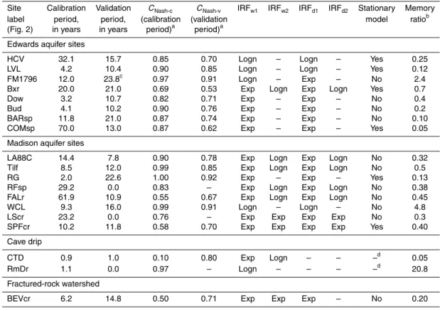
fluctuation amplitudes might be small in comparison to the overall record. Because parameters were optimized for the calibration periods only, CNash-c values were 0.03 higher (4 %) on average thanCNash-vvalues.

Primary and secondary IRFs were included in the initial model calibration for all sites. Trial and error was used to determine whether to use exponential or lognormal IRFs

5

(Table 4). Multiple trials of the calibration process indicated whether or not secondary IRFs were necessary. For example, initial calibration sometimes resulted in a small or negligible curve area for a secondary IRF. In these cases, the minimized IRF was omit-ted if it did not degrade theCNash-v value. In some cases, omitting secondary IRFs re-sulted in increasedCNash-vvalues, which indicated that adding secondary IRFs resulted

10

in overparameterization. For example, using all four IRFs for the Medina FM1796 well resulted in aCNash-vvalue of 0.81, but using only two IRFs resulted in a higherCNash-v value (0.91; Table 4), even though the two cases fit the calibration period equally well.

All models were assumed to be nonstationary for initial calibration trials. Similar shapes for the wet-period and dry-period IRFs indicated that the system might be

sta-15

tionary. Stationarity for these cases was tested by using the same IRF for wet and dry periods. IfCNash-v decreased by less than 0.02 as a result, then parsimony was pre-ferred, and the system was simulated as stationary. In some cases, model fit for the validation period indicated that a stationary model was best. For example,CNash-v for the Lovelady well model was 0.69 for the nonstationary case and 0.85 (Table 4) for the

20

stationary case, which indicated that the nonstationary model was overparameterized.

3.4 Assessing model fit and predictive strength

The length of the validation period is an indicator of the length of time for which a model can be projected with confidence into the future on the basis of climate-model predic-tions. The value of CNash-v is an indicator of the expected model error for the future

25

(16)

HESSD

9, 9577–9609, 2012

karst aquifers

Title Page

Tables Figures

◭ ◮

Back Close

Full Screen / Esc

Discussion

P

a

per

|

Dis

cussion

P

a

per

|

Discussion

P

a

per

|

Discussio

n

P

a

per

|

CNash-v increases with an increasing calibration period, which decreases the length of

the validation period. This inverse relation betweenCNash-vand validation period length results in a compromise that must be considered when setting a targetCNash-v. Also, for nonstationary systems, the calibration periods needed to include both wet and dry periods. Therefore, the length of the validation period was limited in some cases by the

5

occurrence of wet and dry periods for a particular system.

A targetCNash-vvalue was set at 0.70. Three of the sites had very lowCNash-vvalues (<0.5) for any validation-period length tested, and thus this period was set to zero with

no CNash-v value listed (Table 4). Three other sites had CNash-v values that were less

than the target (Table 4). These sites also hadCNash(full period) values that were less

10

than the target, and thus achieving the targetCNash-vwas not possible for any validation period for these sites. TheCNash-vvalue for the remaining sites ranged from 0.70 to 0.92 (Table 4).

An additional measure of predictive strength is the memory ratio, defined as the ratio of the system memory to the length of the period of record for the system response.

15

A value of less than unity for the memory ratio is desirable because if the system memory is longer than the data record, then the IRF has a partial tail segment that has no effect on the model output for the period of record. This means that this tail segment has not been calibrated to data, and model predictions are less certain than if the entire IRF were calibrated. Two sites, Windy City Lake and the Medina FM1796

20

well, had memory ratios greater than unity (Table 4); a memory ratio greater than unity is common for systems such as these with long memories.

Most of the sites were simulated as nonstationary (Table 4), and model spin-up pe-riods were at least as long as system memories for all sites. For Windy City Lake, Medina FM1796 well, and Fall River, data were not available for the first part of the

25

(17)

HESSD

9, 9577–9609, 2012

karst aquifers

Title Page

Tables Figures

◭ ◮

Back Close

Full Screen / Esc

Discussion

P

a

per

|

Dis

cussion

P

a

per

|

Discussion

P

a

per

|

Discussio

n

P

a

per

|

by replacing the mean values with the subsequent period of data, which changed the

CNash-vvalues by less than 0.02 for these three sites. This indicates model insensitivity

to precipitation and temperature variability in the early parts of the spin-up periods.

3.5 Classification of site responses

The eight Edwards aquifer sites and eight Madison aquifer sites were included in PCA

5

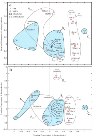
and cluster analysis. Characteristics of the IRF shapes were quantified by 15 metrics (Table 2). The values were log transformed and standardized to a mean of zero and standard deviation of unity before applying PCA. Principal components 1 through 4 (PC1–PC4) explain 50, 18, 14, and 10 %, respectively (92 % total) of the variance in the dataset and represent the primary characteristics quantified by the IRF metrics.

10

The relation of the sites (also known as scores) to the metrics (also known as loadings) were plotted in principal component space (Fig. 4).

Cluster analysis was used to determine similarities between sites and to character-ize site clusters according to the metrics (Fig. 4). First, a cluster analysis was applied to determine site clusters, in which the score values from PCA were used as input for

15

the cluster analysis, as described by Suk and Lee (1999). This analysis iteratively as-signs each site to a cluster by minimizing the sum of Euclidian distances in principal component space between sites (score values) and the nearest cluster centroid (Se-ber, 1984; Spath, 1985). A second cluster analysis was applied to the log-transformed and standardized metric values, with three clusters specified for each analysis. The site

20

clusters primarily are separated on the PC1 axis but occupy similar ranges on the PC2 and PC3 axes, which indicates that PC1 represents the differentiation of the site clus-ters (Fig. 4). The distribution of the plotting positions of sites results from differences in IRF shapes, and the plotting positions of the metrics in relation to the sites reveal specific IRF characteristics that are represented by each principal component.

25

(18)

HESSD

9, 9577–9609, 2012

karst aquifers

Title Page

Tables Figures

◭ ◮

Back Close

Full Screen / Esc

Discussion

P

a

per

|

Dis

cussion

P

a

per

|

Discussion

P

a

per

|

Discussio

n

P

a

per

|

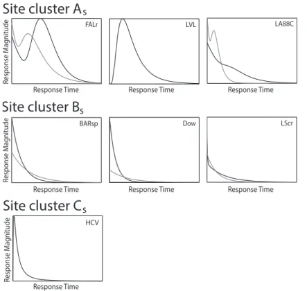
results in a bimodal distribution, and, on average, 68 % of the IRF curve area is log-normal (Fig. 5). Site cluster Bs is typified primarily by an immediate peak response (exponential curve sometimes combined with lognormal), and, on average, 71 % of the IRF curve area is exponential (Fig. 5). Site clusterCscontains only one site (HCV), and the response is 100 % lognormal, with less delay in the lognormal peak than those of

5

site clusterAs(Fig. 5).

The plotting positions of the metrics help explain the meaning of the first three prin-ciple components (Fig. 4). The three metric clusters each occupy a di_fferent range on the PC1 axis and primarily are separated on that axis; on the PC2 and PC3 axes, however, metric clustersAm and Cm occupy largely coincident ranges (Fig. 4). Metric

10

clusterBmis widely separated from the other two on the PC3 axis (Fig. 4). Metrics that are most heavily loaded on PC1 are the mean : memory ratios (MnMm; negative) and all metrics in clusterCm (positive). Thus, these metrics have the largest role in diff er-entiating sites along the PC1 axis and range from sites that have large mean : memory ratios on the left side of Fig. 4 to sites with large skewness and kurtosis (skw, krt) on

15

the right side. The four metrics for skewness and kurtosis (cluster Cm) plot close to one another (Fig. 4a), which indicates positive correlation of these metrics because highly skewed exponential and lognormal curves generally have high kurtosis as well. The other four metrics in clusterCm (deviation : memory (SDMm), standard-deviation : mean (SDMn)) plot in a similar range on PC1 to skewness and kurtosis but

20

in a different range on PC2 (Fig. 4a); thus PC1 makes little distinction between met-rics in clusterCm, whereas PC2 describes these differences. The most heavily loaded metrics on PC2 are the mode : memory ratios (MdMm) and kurtosis (Fig. 4a). The dis-tribution of sites along the PC2 axis range from those with high mode : memory ratios and kurtosis in the upper part to those with high standard-deviation : mean and

peak-25

height : area ratios (PHA) in the lower part (Fig. 4a). Kurtosis is heavily loaded on PC1 and PC2.

(19)

HESSD

9, 9577–9609, 2012

karst aquifers

Title Page

Tables Figures

◭ ◮

Back Close

Full Screen / Esc

Discussion

P

a

per

|

Dis

cussion

P

a

per

|

Discussion

P

a

per

|

Discussio

n

P

a

per

|

these metrics. The distribution of sites along the PC3 axis range from those with high peak-height : area ratios on the upper side to those with high wet : dry area ratios (WDA) on the lower side (Fig. 4b). For PC3, the manner in which metrics in cluster Cm are paired by proximity suggests that PC3 differentiates wet- and dry-period IRFs; i.e., some wet-period metrics and dry-period metrics are paired on PC3 (skw-w and

5

krt-w, skw-d and krt-d, SDMn-w and SDMm-w, SDMn-d and SDMm-d; Fig. 4b). This pairing also indicates a separation between the wet and dry counterparts of these met-rics; e.g., skw-w and kurt-w are paired, but skw-w and skw-d are separated (Fig. 4b). Further, the wet and dry counterparts of the mode : memory ratio plot farthest apart on PC3 (Fig. 4).

10

The wet : dry area ratio is the most heavily loaded metric on PC4 (not shown), which indicates that PC4 primarily describes this metric. Therefore, PC4 also represents dif-ferences between wet and dry periods, except that PC4 is associated with differences in IRF area rather than shape.

Six of the 16 Edwards and Madison aquifer sites (38 %) are stationary (Table 4),

15

which caused the wet and dry metric counterparts to plot more closely on Fig. 4 than if all sites were nonstationary. Positively correlated metrics are easily identified by prox-imity of plotting position, whereas negatively correlated metrics can be identified as those that plot on opposite sides of the origin; e.g., MnMm and SDMn (Fig. 4a).

4 Conclusions

20

The convolution models are well suited to link climate scenarios to hydrologic re-sponses critical to human water supply and ecosystems. As climate models improve in simulating storm processes, projected precipitation and air-temperature recoreds can be used as input for hydrologic models to investigate how water levels and spring discharge might change. The output from the hydrologic models can, in turn,

25

(20)

HESSD

9, 9577–9609, 2012

karst aquifers

Title Page

Tables Figures

◭ ◮

Back Close

Full Screen / Esc

Discussion

P

a

per

|

Dis

cussion

P

a

per

|

Discussion

P

a

per

|

Discussio

n

P

a

per

|

(e.g., three-dimensional finite difference), convolution models are calibrated to data at short time steps that are well suited to short-term variability characteristic of karst groundwater responses.

The use of multiple metrics to describe the IRFs provides a novel way to characterize and compare the way in which multiple sites respond to recharge. Classification of the

5

IRF metrics and evaluation with PCA and cluster analysis indicate that there is a range of IRF characteristics describing different sites within a karst system. The IRF shape is a result of the aquifer’s pore geometry and connectivity, which is spatially heteroge-neous in karst aquifers, and thus similar site types do not necessarily display similar IRFs. Knowing which metrics correspond to the different principle components assists

10

in understanding the meaning of these components hydrologically. This understanding also requires an understanding of how each metric affects the shape of the IRF and what the IRF shapes mean hydrologically.

Two of the site clusters contain sites for both aquifers (clusterCs contains only one site), and site cluster Bs, which contains most of the sites, is equally balanced

be-15

tween the two aquifers. This indicates that the differences that exist within either aquifer are larger than the differences between the two aquifers and that these two aquifers are similar according to this classification. The Madison and Edwards aquifers each have well-developed networks of large conduits, which is consistent with the similar-ity determined by the classification. Currently, IRFs have been developed for only two

20

karst aquifers, but as convolution models are developed for additional sites in additional aquifers, they could contribute to an IRF database and, moreover, a general classifica-tion system for karst aquifers. Of particular interest will be comparison of telogenetic and eogenetic systems, humid and arid systems, and diffuse- and conduit-controlled systems. The availability of long-term records for precipitation, air temperature, water

25

(21)

HESSD

9, 9577–9609, 2012

karst aquifers

Title Page

Tables Figures

◭ ◮

Back Close

Full Screen / Esc

Discussion

P

a

per

|

Dis

cussion

P

a

per

|

Discussion

P

a

per

|

Discussio

n

P

a

per

|

Supplementary material related to this article is available online at: http://www.hydrol-earth-syst-sci-discuss.net/9/9577/2012/

hessd-9-9577-2012-supplement.zip.

Acknowledgements. The authors would like to thank Johnathan Bumgarner of the US Geolog-ical Survey for his helpful review and comments on an early draft of this article. We also thank

5

Jonathan McKaskey, Thomas Sample, and Jennifer Bednar of the US Geological Survey for assistance with obtaining data and creating figures and tables.

References

Back, W., Hanshaw, B. B., Plummer, L. N., Rahn, P. H., Rightmire, C. T., and Rubin, M.: Process and rate of dedolomitization: mass transfer and 14C dating in a regional carbonate aquifer,

10

Geol. Soc. Am. Bull., 94, 1415–1429, 1983.

Coleman, T. F. and Li, Y.: On the convergence of reflective newton methods for large-scale nonlinear minimization subject to bounds, Math. Program., 67, 189–224, 1994.

Coleman, T. F. and Li, Y.: An interior, trust region approach for nonlinear minimization subject to bounds, SIAM J. Optimiz., 6, 418–445, 1996.

15

Covington, M. D., Wicks, C. M., and Saar, M. O.: A dimensionless number describing the effects of recharge and geometry on discharge from simple karstic aquifers, Water Resour. Res., 45, 1–16, 2009.

Covington, M. D., Luhmann, A. J., Wicks, C. M., and Saar, M. O.: Process length scales and longitudinal damping in karst conduits, J. Geophys. Res.-Earth, 117, F01025,

20

doi:10.1029/2011JF002212, 2012.

Davis, J. C.: Statistics and Data Analysis in Geology, John Wiley & Sons, Inc., Hoboken, New Jersey, 2002.

Denić-Jukić, V. and Jukić, D.: Composite transfer functions for karst aquifers, J. Hydrol., 274, 80–94, 2003.

25

(22)

HESSD

9, 9577–9609, 2012

karst aquifers

Title Page

Tables Figures

◭ ◮

Back Close

Full Screen / Esc

Discussion

P

a

per

|

Dis

cussion

P

a

per

|

Discussion

P

a

per

|

Discussio

n

P

a

per

|

Greene, E. A. and Rahn, P. H.: Localized anisotropic transmissivity in a karst aquifer, Ground Water, 33, 806–816, 1995.

Hall, F. R. and Moench, A. F.: Application of the convolution equation to stream–aquifer rela-tionships, Water Resour. Res., 8, 487–493, 1972.

Hortness, J. E. and Driscoll, D. G.: Streamflow Losses in the Black Hills of Western South

5

Dakota, US Geol. Surv., Reston, VA, WRIR 98–4116, 99 pp., 1998.

Hostetler, S. W., Alder, J. R., and Allan, A. M.: Dynamically Downscaled Climate Simulations over North America: Methods, Evaluation and Supporting Documentation for Users, US Geol. Surv., Reston, VA, 64 pp., 2011.

Jakeman, A. J. and Hornberger, G. M.: How much complexity is warranted in a rainfall-runoff

10

model?, Water Resour. Res., 29, 2637–2649, 1993.

Jeannin, P. Y.: Modeling flow in phreatic and epiphreatic karst conduits in the H ¨olloch cave (Muotatal, Switzerland), Water Resour. Res., 37, 191–200, 2001.

Jukić, D. and Denić-Jukić, V.: Nonlinear kernel functions for karst aquifers, J. Hydrol., 328, 360– 374, 2006.

15

Jukić, D. and Denić-Jukić, V.: Partial spectral analysis of hydrological time series, J. Hydrol., 400, 223–233, 2011.

Labat, D., Masbou, J., Beaulieu, E., and Mangin, A.: Scaling behavior of the fluctuations in stream flow at the outlet of karstic watersheds, France, J. Hydrol., 410, 162–168, 2011. Lindgren, R. J., Dutton, A. R., Hovorka, S. D., Worthington, S. R. H., and Painter, S.:

Conceptu-20

alization and Simulation of the Edwards Aquifer, San Antonio Region, Texas, US Geol. Surv., Reston, VA, SIR 2004–5277, 154 pp., 2005.

Lo ´aiciga, H. A., Maidment, D. R., and Valdes, J. B.: Climate-change impacts in a regional karst aquifer, J. Hydrol., 227, 173–194, 2000.

Long, A. J.: Hydrograph separation for karst watersheds using a two-domain rainfall-discharge

25

model, J. Hydrol., 364, 249–256, 2009.

Long, A. J. and Derickson, R. G.: Linear systems analysis in a karst aquifer, J. Hydrol., 219, 206–217, 1999.

Long, A. J. and Putnam, L. D.: Translating CFC-based piston ages into probability density func-tions of ground-water age in karst, J. Hydrol., 330, 735–747, 2006.

30

(23)

HESSD

9, 9577–9609, 2012

karst aquifers

Title Page

Tables Figures

◭ ◮

Back Close

Full Screen / Esc

Discussion

P

a

per

|

Dis

cussion

P

a

per

|

Discussion

P

a

per

|

Discussio

n

P

a

per

|

Mearns, L. O., Gutowski, W. J., Jones, R., Leung, L. Y., McGinnis, S., Nunes, A. M. B., and Qian, Y.: A regional climate change assessment program for North America, EOS T. Am. Geophys. Un., 90, 311–312, 2009.

Miller, L. D. and Driscoll, D. G.: Streamflow Characteristics for the Black Hills of South Dakota, Through Water Year 1993, US Geol. Surv., Reston, VA, SIR 97–4288, 322 pp., 1998.

5

Nash, J. E. and Sutcliffe, J. V.: River flow forecasting through conceptual models part I – a dis-cussion of principles, J. Hydrol., 10, 282–290, 1970.

National Climatic Data Center: National Oceanic and Atmospheric Administration, US Depart-ment of Commerce, available at: http://www.ncdc.noaa.gov, last access: 14 June 2012. Olsthoorn, T. N.: Do a bit more with convolution, Ground Water, 46, 13–22, 2008.

10

Pinault, J. L., Plagnes, V., Aquilina, L., and Bakalowicz, M.: Inverse modeling of the hydro-logical and the hydrochemical behavior of hydrosystems; characterization of karst system functioning, Water Resour. Res., 37, 2191–2204, 2001.

Rahn, P. H. and Gries, J. P.: Large springs in the Black Hills, South Dakota and Wyoming, in: Report of Investigations – Department of Natural Resource Development, South Dakota

Ge-15

ological Survey, 107, 100 pp., 1973.

Reimann, T., Geyer, T., Shoemaker, W. B., Liedl, R., and Sauter, M.: Effects of dynamically variable saturation and matrix-conduit coupling of flow in karst aquifers, Water Resour. Res., 47, W11503, doi:10.1029/2011WR010446, 2011.

Seber, G. A. F.: Multivariate Observations, John Wiley & Sons, Inc., Hoboken, New Jersey,

20

1984.

Simoni, S., Padoan, S., Nadeau, D. F., Diebold, M., Porporato, A., and Barrentxea, G.: Hy-drologic response of an alpine watershed: application of a meteorological wireless sen-sor network to understand streamflow generation, Water Resour. Res., 47, W10524, doi:10.1029/2011WR010730, 2011.

25

Singh, V. P.: Hydrologic Systems: Rainfall-RunoffModeling, Prentice Hall, Englewood Cliffs, NJ, 1988.

Small, T. A., Hanson, J. A., and Hauwert, N. M.: Geologic Framework and Hydrogeologic Characteristics of the Edwards Aquifer Outcrop (Barton Springs Segment), Northeastern Hays and Southwestern Travis Counties, Texas, US Geol. Surv., Denver, CO, WRIR96-4306,

30

15 pp., 1996.

(24)

HESSD

9, 9577–9609, 2012

karst aquifers

Title Page

Tables Figures

◭ ◮

Back Close

Full Screen / Esc

Discussion

P

a

per

|

Dis

cussion

P

a

per

|

Discussion

P

a

per

|

Discussio

n

P

a

per

|

Spath, H.: Cluster Dissection and Analysis: Theory, FORTRAN Programs, Examples, Halsted Press, New York, 1985.

Suk, H. and Lee, K. K.: Characterization of a ground water hydrochemical system through multivariate analysis: clustering into ground water zones, Ground Water, 37, 358–366, 1999. US Geological Survey, National Water Information System (NWISWeb): US Geological Survey

5

database, available at: IRFmetricsindicatethattherehttp://waterdata.usgs.gov/usa/nwis/nwis, last access: 14 June 2012.

(25)

HESSD

9, 9577–9609, 2012

karst aquifers

Title Page

Tables Figures

◭ ◮

Back Close

Full Screen / Esc

Discussion

P

a

per

|

Dis

cussion

P

a

per

|

Discussion

P

a

per

|

Discussio

n

P

a

per

|

Table 1.Model parameters.

Parameter Description Equation Estimation method

c Soil moisture parameter 1 Optimized

κ Soil moisture parameter 3 Optimized

f Soil moisture parameter 3 Optimized

λ Exponential IRF shape parameter 7 Optimized

a Exponential IRF curve area 7 Optimized

ω Lognormal IRF shape parameter 10 Optimized

ε Lognormal IRF shape parameter 10 Optimized

b Lognormal IRF curve area 10 Optimized

S_f Sublimation fraction –∗ _Optimized

h₀ Hydraulic-head datum –∗ _Optimized

T_s Snow precipitation threshold –∗ _{Assumed 0}◦_C

T_m Snowmelt threshold –∗ _Empirical

(26)

HESSD

9, 9577–9609, 2012

karst aquifers

Title Page

Tables Figures

◭ ◮

Back Close

Full Screen / Esc

Discussion

P

a

per

|

Dis

cussion

P

a

per

|

Discussion

P

a

per

|

Discussio

n

P

a

per

|

Table 2.Impulse-response function (IRF) metrics. Metrics were quantified for wet and dry

peri-ods separately by adding “-w” or “-d”, respectively, to the abbreviations.

IRF Metric Abbreviation

Skewness skw

Kurtosis krt

SD : mean ratio SDMn

SD : memory ratio SDMm

Mean : memory ratio MnMm

Mode : memory ratio MdMm

Peak-height : area ratio PHA

Wet : dry area ratio WDA∗

(27)

HESSD

9, 9577–9609, 2012

karst aquifers

Title Page

Tables Figures

◭ ◮

Back Close

Full Screen / Esc

Discussion

P

a

per

|

Dis

cussion

P

a

per

|

Discussion

P

a

per

|

Discussio

n

P

a

per

|

Table 3.Sites simulated

Site label (Fig. 2) Site name USGS site numbera Site type Edwards aquifer sites

FM1796 Medina FM1796 292618099165901 Well Bxr Bexar Co. Index well 292845098255401 Well HCV Hill Country Village 293522098291201 Well Bud Buda Well 300510097504001 Well Dow Dowell Well 300835097483401 Well BARsp Barton Springs 8155500 Spring

LVL Lovelady 8159000 Well

COMsp Comal Spring 8168710 Spring

Madison aquifer sites

FALr Fall River 06402000 Spring complex RFsp Rhoads Fork Spring 06408700 Spring

LScr Little Spearfish Creek 06430850 Base flow SPFcr Spearfish Creek 06430900 Base flow WCL Windy City Lake 433302103281501b Cave water body RG Reptile Gardens wellc 435916103161801 Well

Tilf Tilford well 441759103261202 Well LA88C Spearfish GC well 442854103505602 Well Cave drip

CTD Caving Tour drip 433302103281508d Cave drip RmDr Room Draculum drip 433302103281509d Cave drip Fractured-rock watershed

BEVcr Beaver Creek 06402430 Watershed

a

Flow and water-level data from US Geological Survey (2012) unless otherwise indicated.

b_{Partial water-level record was estimated from water levels in well Md7-11 (Fig. 2) with data from the South Dakota Department of the} Environment and Natural Resources in Pierre, South Dakota (R2=0.99 for correlation between the two sites; Davis, 2002). c

(28)

HESSD

9, 9577–9609, 2012

karst aquifers

Title Page

Tables Figures

◭ ◮

Back Close

Full Screen / Esc

Discussion

P

a

per

|

Dis

cussion

P

a

per

|

Discussion

P

a

per

|

Discussio

n

P

a

per

|

Table 4.Summary of modeling results.

Site Calibration Validation CNash-c CNash-v IRFw1 IRFw2 IRFd1 IRFd2 Stationary Memory

label period, period, (calibration (validation model ratiob

(Fig. 2) in years in years period)a period)a Edwards aquifer sites

HCV 32.1 15.7 0.85 0.70 Logn – Logn – Yes 0.25

LVL 4.2 10.4 0.90 0.85 Logn – Logn – Yes 0.12

FM1796 12.0 23.8c 0.97 0.91 Logn – Exp – No 2.4

Bxr 20.0 21.0 0.69 0.53 Exp Logn Exp Logn Yes 0.7

Dow 3.2 10.7 0.82 0.71 Exp – Exp – No 0.4

Bud 4.1 10.2 0.90 0.76 Exp – Exp – No 0.2

BARsp 11.8 21.0 0.87 0.74 Exp – Exp – No 0.10

COMsp 70.0 13.0 0.87 0.62 Exp – Exp – Yes 0.05

Madison aquifer sites

LA88C 14.4 7.8 0.90 0.78 Exp Logn Exp Logn No 0.32

Tilf 8.5 12.0 0.99 0.85 Exp Logn Exp Logn No 0.5

RG 2.0 22.6 1.00 0.92 Exp – Exp – Yes 0.13

RFsp 29.2 0.0 0.83 – Exp Logn Exp Logn No 0.38

FALr 61.9 10.9 0.55 0.67 Exp Logn Exp Logn No 0.45

WCL 9.3 16.0 0.99 0.91 Logn – Logn – No 4.8

LScr 23.2 0.0 0.76 – Exp Exp Exp Exp No 0.3

SPFcr 10.2 11.8 0.58 0.70 Exp Exp Exp Exp Yes 0.40

Cave drip

CTD 0.9 1.0 0.10 0.80 Exp Logn – – –d 0.05

RmDr 1.1 0.0 0.97 – Logn – – – –d 20.8

Fractured-rock watershed

BEVcr 6.2 14.8 0.50 0.71 Exp Exp Exp – No 0.20

IRF, impulse-response function; w1, wet period primary; w2, wet period secondary; d1, dry period primary; d2, wet period secondary; Exp, exponential curve; Logn, lognormal curve; –, not applicable.

a_{Dimensionless; computed on a daily time step.}

b_{Ratio of system memory to full system-response period, dimensionless.} c_{Also includes a backward validation period of 12.5 yr.}

(29)

HESSD

9, 9577–9609, 2012

karst aquifers

Title Page

Tables Figures

◭ ◮

Back Close

Full Screen / Esc

Discussion

P

a

per

|

Dis

cussion

P

a

per

|

Discussion

P

a

per

|

Discussio

n

P

a

per

|

a

Primary IRF (exponential)

Secondary IRF (lognormal)

Compound IRF

Response Time

Response mag

nitude

c

Secondary IRF (exponential)

d b

Response mag

nitude

Primary IRF (exponential)

Compound IRF

Response Time

Fig. 1.Examples of compound impulse-response functions (IRFs) consisting of the

(30)

HESSD

9, 9577–9609, 2012

karst aquifers

Title Page

Tables Figures

◭ ◮

Back Close

Full Screen / Esc

Discussion

P

a

per

|

Dis

cussion

P

a

per

|

Discussion

P

a

per

|

Discussio

n

P

a

per

|

"

Austin

San Antonio Bud

Bex

LVL

COMsp BARsp

FM1796

DOW

HCV

98°0'0"W 99°0'0"W

100°0'0"W

31°0'0"N

30°0'0"N

29°0'0"N

" " "

"

Md7-11 Spearfish

Rapid City

Hot Springs RG

CTD

WCL RmDr LScr

FALr RFsp

Tilf SPFcr

LA88C

103°0'0"W 104°0'0"W

44°0'0"N 44°20'0"N

43°40'0"N

EXPLANATION

Madison aquifer surface recharge area

Madison aquifer below land surface (confined)

Edwards aquifer surface recharge area

Edwards aquifer below land surface (confined)

Hydrologic observation site (simulated)

City

Madison aquifer

Edwards aquifer

# Streamflow gage

#

06407500

Observation well

(31)

HESSD

9, 9577–9609, 2012

karst aquifers

Title Page

Tables Figures

◭ ◮

Back Close

Full Screen / Esc

Discussion

P

a

per

|

Dis

cussion

P

a

per

|

Discussion

P

a

per

|

Discussio

n

P

a

per

|

1976 1978 1980 1982 1984 1986 1988 1990 1992 1994 1996 1998 2000 2002 2004 2006 2008 2010 2012 0

1 2 3 4 5

Time

Flow, in m /s

Observed Simulated

Calibration period Validation period

3