Similarity estimators for irregular and age uncertain time series

(1)

CPD

9, 5299–5346, 2013

Similarity estimators

K. Rehfeld and J. Kurths

Title Page

Abstract Introduction

Conclusions References

Tables Figures

◭ ◮

Back Close

Full Screen / Esc

Printer-friendly Version Interactive Discussion

Discussion

P

a

per

|

Dis

cussion

P

a

per

|

Discussion

P

a

per

|

Discussio

n

P

a

per

|

Clim. Past Discuss., 9, 5299–5346, 2013 www.clim-past-discuss.net/9/5299/2013/ doi:10.5194/cpd-9-5299-2013

Open Access

Climate of the Past

Discussions

Geoscientiic Geoscientiic

This discussion paper is/has been under review for the journal Climate of the Past (CP). Please refer to the corresponding final paper in CP if available.

Similarity estimators for irregular and age

uncertain time series

K. Rehfeld1,2and J. Kurths1,2,3

1

Potsdam Institute for Climate Impact Research, P.O. Box 601203, 14412 Potsdam, Germany

2

Department of Physics, Humboldt-Universit ¨at zu Berlin, Newtonstr. 15, 12489 Berlin, Germany

3

Institute for Complex Systems and Mathematical Biology, University of Aberdeen, Aberdeen, AB243UE, UK

Received: 15 August 2013 – Accepted: 4 September 2013 – Published: 16 September 2013

Correspondence to: K. Rehfeld ([email protected])

Published by Copernicus Publications on behalf of the European Geosciences Union.

(2)

CPD

9, 5299–5346, 2013

Title Page

Tables Figures

◭ ◮

Back Close

Full Screen / Esc

Discussion

P

a

per

|

Dis

cussion

P

a

per

|

Discussion

P

a

per

|

Discussio

n

P

a

per

|

Abstract

Paleoclimate time series are often irregularly sampled and age uncertain, which is an important technical challenge to overcome for successful reconstruction of past climate variability and dynamics. Visual comparison and interpolation-based linear correlation approaches have been used to infer dependencies from such proxy time series. While

5

the first is subjective, not measurable and not suitable for the comparison of many datasets at a time, the latter introduces interpolation bias, and both face difficulties if the underlying dependencies are nonlinear.

In this paper we investigate similarity estimators that could be suitable for the quan-titative investigation of dependencies in irregular and age uncertain time series. We

10

compare the Gaussian-kernel based cross correlation (gXCF, Rehfeld et al., 2011) and mutual information (gMI, Rehfeld et al., 2013) against their interpolation-based counter-parts and the new event synchronization function (ESF). We test the efficiency of the methods in estimating coupling strength and coupling lag numerically, using ensem-bles of synthetic stalagmites with short, autocorrelated, linear and nonlinearly coupled

15

proxy time series, and in the application to real stalagmite time series.

In the linear test case coupling strength increases are identified consistently for all estimators, while in the nonlinear test case the correlation-based approaches fail. The lag at which the time series are coupled is identified correctly as the maximum of the similarity functions in around 60–55 % (in the linear case) to 53–42 % (for the nonlinear

20

processes) of the cases when the dating of the synthetic stalagmite is perfectly pre-cise. If the age uncertainty increases beyond 5 % of the time series length, however, the true coupling lag is not identified more often than the others for which the similarity function was estimated. Age uncertainty contributes up to half of the uncertainty in the similarity estimation process. Time series irregularity contributes less, particularly for

25

the adapted Gaussian-kernel based estimators and the event synchronization function. The introduced link strength concept summarizes the hypothesis test results and bal-ances the individual strengths of the estimators: while gXCF is particularly suitable for

(3)

CPD

9, 5299–5346, 2013

Title Page

Tables Figures

◭ ◮

Back Close

Full Screen / Esc

Discussion

P

a

per

|

Dis

cussion

P

a

per

|

Discussion

P

a

per

|

Discussio

n

P

a

per

|

short and irregular time series, gMI and the ESF can identify nonlinear dependencies. ESF could, in particular, be suitable to study extreme event dynamics in paleoclimate records. Programs to analyze paleoclimatic time series for significant dependencies are included in a freely available software toolbox.

1 Introduction

5

Time series are often used to assess the properties of the processes that generated them, in climate science (Rehfeld et al., 2011) but also in many other scientific fields ranging from ecology (Lhermitte et al., 2011) to astrophysics (Scargle, 1989). Time series similarity measures quantify the degree of statistical association and are, par-ticularly in the geoscientific context, often equated with Pearson correlation (Chatfield,

10

2004). They help to identify the strength of dependencies between climate processes and potential lead/lag relationships. For modern-day weather stations, both daily tem-perature and the time of observations are logged precisely. To identify relationships between distant weather evolution, time series of temperature anomalies can be com-pared. Paleoclimate data are crucial to investigate climate inter-relationships beyond

15

the instrumental record. Paleoclimate time series are, however, more challenging than the data sources in other disciplines: Neither observation time nor the climatic vari-able are known precisely. Both have to be reconstructed, resulting in irregular and age uncertain time series, because variability in the growth of the archive impacts on the temporal resolution of the resulting proxy time series (Fig. 1). The dependency of

re-20

constructed paleoclimate time series, and its relationship to global or external forcing, is often inferred from similarities, coinciding maxima/minima or trends, between graph-ical visualizations of the time series (for example in Zhang et al., 2008; Cheng et al., 2012; Sinha et al., 2011; Zhang et al., 2011). Visual comparison is, however, inherently subjective, can not be quantified and tested in a hypothesis test and will not suffice with

25

the growing number of paleoclimatic datasets available.

(4)

CPD

9, 5299–5346, 2013

Title Page

Tables Figures

◭ ◮

Back Close

Full Screen / Esc

Discussion

P

a

per

|

Dis

cussion

P

a

per

|

Discussion

P

a

per

|

Discussio

n

P

a

per

|

Standard statistical techniques, such as estimating the Pearson correlation (XC), can not readily be applied when the sampling of the time series is irregular. XC is, in prin-ciple, computed by taking the arithmetic mean over the products of coeval, centralized and standardized observations and reflects the goodness of a linear fit to the scatter-plot of the data. If the two time series to be correlated are irregular, coeval observations

5

are only given in the special case that both time series have the same timescale. In practice, this would arise only if, for example, two proxies were measured on the same samples. In the general case the irregularity precludes the direct computation. Inter-polating the time series to a regular coinciding timescale, however, results in a loss of high-frequency variability and a spectral bias towards low frequencies (Schulz and

10

Stattegger, 1997). In a comparison of correlation analysis techniques the Gaussian-kernel-based Pearson correlation was identified as a reliable and robust estimator for irregular time series (Rehfeld et al., 2011). However, relationships in the climate sys-tem are not always linear, and therefore not necessarily identifiable by linear techniques such as Pearson correlation. This is not a problem in the geosciences alone, and

simi-15

larity measures that can capture nonlinear inter-relationships exist. Mutual Information (MI), an entropy-based measure, has been used to investigate nonlinear dependencies of processes from observations (Donges et al., 2009; Runge et al., 2012; Hlinka et al., 2013). In this measure, the joint and marginal distributions of processesX andY are evaluated. Its advantage is that it is model-free and able to quantify nonlinear

depen-20

dencies, but it is symmetric, MI(X, Y)=MI(−X, Y), and more difficult to quantify as the quantification bias changes considerably for different sample sizes and estimator techniques (Khan et al., 2007; Kraskov et al., 2004). It has been adapted and tested for irregular and autocorrelated time series (Rehfeld et al., 2013) in a Gaussian-kernel-based variant. Both MI and XC depend on the notion of a scatterplot between the data.

25

An alternative, especially in the analysis of extreme events, could be found in the mea-sure of Event Synchronization (ES, Quian Quiroga et al., 2002), which is not based on the available time series, but the relative timing of distinguished events in two time series. Originally conceived for neurophysiological signals, it has become a popular

(5)

CPD

9, 5299–5346, 2013

Title Page

Tables Figures

◭ ◮

Back Close

Full Screen / Esc

Discussion

P

a

per

|

Dis

cussion

P

a

per

|

Discussion

P

a

per

|

Discussio

n

P

a

per

|

measure to investigate dependencies in precipitation time series (Malik et al., 2010, 2011; Rheinwalt et al., 2012), but it has not been tested for its suitability on short and autocorrelated time series. In its original form it provides a measure for the strength of synchronization and for the direction of a potential coupling between the processes generating the events, but not for the lag of the potential coupling. Although stated

5

differently in the original paper, ES does not require regular observation intervals. A number for an individual correlation coefficient can be interpreted, when its level of significance is determined as well. For the usually short and autocorrelated paleocli-matic time series, this can be done by bootstrapping the result (Mudelsee, 2002), or by testing the similarity for uncorrelated surrogate time series with similar autocorrelation

10

properties (Rehfeld et al., 2011, 2013). The values of the di_fferent estimators, however, can not be compared directly, as they vary on different scales. In this paper we eval-uate the impact of age uncertainty and time series irregularity on the accuracy of the estimators.

Furthermore we propose the concept of alink strength, to summarize the hypothesis

15

test results of different estimators. If no outcome is significant, it is zero, if three out of five employed estimators yield a significant similarity, the link strength is 3₅ and if all tests for null correlation were rejected the link strength is equal to unity. The advantage of this approach lies in its robustness due to the different estimators, and in the easy consideration of uncertain datasets. If the uncertainty of the time series can be

mod-20

eled, for example using the Monte Carlo techniques in age modeling software such as StalAge (Scholz and Hoffmann, 2011) or COPRA (Breitenbach et al., 2012), it can be incorporated in the link strength considerations in a straightforward manner.

In this paper we will investigate how well each of these estimators identify the strength and the delay time of actual coupling between paleoclimatic processes from

25

irregular and age uncertain time series. First we review the similarity measures (XC, MI), and develop a Event Synchronization Function (ESF) based on the concept of ES. We simulate artificial stalagmites with linearly and nonlinearly coupled proxy time se-ries based on autoregressive (AR) and threshold-autoregressive (TAR) models. Using

(6)

CPD

9, 5299–5346, 2013

Title Page

Tables Figures

◭ ◮

Back Close

Full Screen / Esc

Discussion

P

a

per

|

Dis

cussion

P

a

per

|

Discussion

P

a

per

|

Discussio

n

P

a

per

|

these and the stalagmite time series from Dandak (Sinha et al., 2011) and Wanxiang (Zhang et al., 2008) cave we investigate how the similarity estimators perform for irreg-ular, age uncertain and autocorrelated time series, and how they are impacted by age uncertainty.

2 Methods

5

In this section we first give necessary definitions for time series and similarity mea-sures, and derive the ESF and the link strength concept.

2.1 Time series

Time series are a collection of measurements of specific properties of an dynamical process, together with the time when the observation (or measurement) took place.

10

The individual data points of the series are often regarded as observations of pro-cesses, which may be deterministic, stochastic, or a combination of both. Economical interests have motivated humans to record, for example, annual wheat prices (as early as 1810 AD), daily stock indices or air temperature (Chatfield, 2004). Stock prices in different markets may be co-dependent, but the reason for similar patterns may not be

15

the same. These processes, named, say,XandY and observed over the timest, yield the time seriesx(t) andy(t). In classical time series analysis the observation times are expected to be regular and certain, and the observation values to be measured exactly, as well.

Definition 1 (Regular time series) The process X_t was observed through the

regu-20

larly sampled time seriesx(t)₌(x_i)_i₌_1,...,N, where the observation times are given by multiplication of the index variablei with the common time step∆t:ti=i∆t+t0.

In contrast to this, for irregular time series no unique sampling rate can be defined, and the observation times cannot be directly related to an index anymore, but have to

(7)

CPD

9, 5299–5346, 2013

Title Page

Tables Figures

◭ ◮

Back Close

Full Screen / Esc

Discussion

P

a

per

|

Dis

cussion

P

a

per

|

Discussion

P

a

per

|

Discussio

n

P

a

per

|

be given explicitly for each measurement. The observation time of irregular time series might even carry some amount of information independently of the observation values, as periods where the number of (reconstructed) observations over time are significantly lower (higher) than others indicate a climate that is unfavorable (favorable) for archive growth.

5

Definition 2 (Irregular time series) An irregular time series x(t)₌(t_i,x_i) is defined by its observation timest_i and the respective observationsx_i, wherei=1, . . . ,N. The two tuples have a common lengthN_x, withtx₁< t₂x<. . . <tx_Nx as observation times.

In the following we focus on the age uncertain paleoclimate proxy time series for which a growth model of the archive has been combined with point-wise age

informa-10

tion, for example from uranium/thorium measurements. Input data to this age modeling are (i) a dating table with its entries containing depths, associated age estimates and their uncertainties, usually given as standard deviations, and (ii) the proxy observa-tions.

Definition 3 (Dating table) A dating tableD=(D_i,T_i,σ_T

i)i=1,...,Ndat containsNdat

point-15

wise age estimatesT_i taken at depthsD_i and their corresponding age standard devia-tionsσ_T

i.

Definition 4 (Proxy observation series) Proxy observation series Xd₌(d_j, x_j) are given forj=1, . . . ,Nobsmeasurement depthsdj and proxy measurementsxj.

Definition 5 (Age model) For paleoclimate archives, the ages at few depths are

esti-20

mated, with some uncertainty. Age models are then created to interpolate from these few dates to a time axis for the proxy time series, which is sampled much more densely in depth than the dating table. Thus, an age model is defined here as one potential depth-age relationshipt_i(z_i)out of the possible ensemble of age modelsT.

For Monte Carlo (MC) age modeling, wholeensemblesof age models,T_{are created,} 25

(8)

CPD

9, 5299–5346, 2013

Title Page

Tables Figures

◭ ◮

Back Close

Full Screen / Esc

Discussion

P

a

per

|

Dis

cussion

P

a

per

|

Discussion

P

a

per

|

Discussio

n

P

a

per

|

usually the most likely age model is selected as the time axis for proxy time series (Breitenbach et al., 2012; Scholz and Ho_ffmann, 2011).

The dating table is combined with the proxy observation series using a single age model and forms a time-uncertain time series.

Definition 6 (Time-uncertain time series) Time-uncertain time series (t_i,x_i,σ_t_i)

as-5

semblei=1, . . . ,N observationsx_i, reconstructed (most probable) observation times

t_i fromTand the observation time uncertaintyσ_t i.

2.2 Estimating similarity of irregular time series

Similar objects agree in some properties, while they may disagree in others. The pop-ular saying “you can not compare apples and oranges”1is misleading in this context,

10

because it implies only that it is not possible to compare them because they are not the exactsametype of objects. It is possible, however, to compare apples and oranges in terms of their weights, glucose content, or environmental footprint, in which they might besimilar ordifferent. Similarity measures, analogously, reflect statistical properties of time series, which may not reflect the same climatic parameters. Different estimators

15

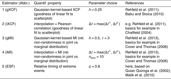
focus on different characteristic properties related to the distributions of the observa-tions, we summarize them in Table 1.

Assume that the processes X and Y generated time series x(t) and y(t). These processes, and the time series, are similar if, for example, coeval minima or maxima were observed. Comparison can then give information about functional relationships

20

between processes underlying time series: Given that two processes X and Y are not independent, there may either be a causal relationship or they are both driven by a globalcommon driver, or there are unobservable intermediate processes, as illus-trated in Fig. 2. A significant similarity estimate may therefore arise for such physical reasons - or as a false positive of the statistical test. If a transfer function between these

25

two processes exists in a form ofYt=F(Xt+ℓ), this results in a repetition of a pattern,

1

Or: apples and pears, in German.

(9)

CPD

9, 5299–5346, 2013

Title Page

Tables Figures

◭ ◮

Back Close

Full Screen / Esc

Discussion

P

a

per

|

Dis

cussion

P

a

per

|

Discussion

P

a

per

|

Discussio

n

P

a

per

|

though maybe distorted, that occurs inX_tatt0and inYtat a timet=t0+ℓ later. A

sim-ilarity estimator can help identify_F and quantifies the similarities in the contemporary evolution of two time series:

Definition 7 (Similarity estimator) A similarity estimatorS=F((tx,x)(ty,y)) reflects the similarity between x(t) and y(t) to a numeric value in an interval [a, b], S:

5

x(t)_×y(t)_→[a,b].

For most similarity measures a=−1, b=1 is considered, but for different estimators different bounds exist. Here we only require that the relationship between true depen-dency and estimated similarity is monotonically increasing. If the delay timeℓ in the transfer function is nonzero, a similarity function gives the similarity between two time

10

series for increasing delay:

Definition 8 (Similarity function) A similarity function S(ℓ)gives the estimated simi-larity over di_fferent lag timesℓ:

S(ℓ) =S(ℓ _·∆t) =f tx,x

, ty ₊ℓ _·∆t,y

. (1)

The spacing of the lag vector is uniform and depends on the mean time resolution

15

of the time series:∆ℓ=max(∆t_x,∆t_y). To indicate that we are focusing on bivariate similarity we also use the alternative notationS(X,Y) which does not explicitly refer to the possible lags.

Similarity measures as required in this context should satisfy at least four properties in an adaptation of the axiomatic definition of Batyrshin et al. (2012):

20

– Symmetry:S(x(t), (t))=S(y(t),x(t))

The statistical association should not change under a permutation of the argu-ments.

– Reflexivity:S(x(t),x(t))=b

When comparing a time series with itself the dependency is always maximal.

25

(10)

CPD

9, 5299–5346, 2013

Title Page

Tables Figures

◭ ◮

Back Close

Full Screen / Esc

Discussion

P

a

per

|

Dis

cussion

P

a

per

|

Discussion

P

a

per

|

Discussio

n

P

a

per

|

– Translation invariance:S(x(t)+c,y(t))=S(x(t),y(t)),c₆=0

Adding or subtracting a constant to one of the time series does not change the resulting estimate.

– Scale invariance:S(ax(t),y(t))=S(x(t),y(t)),a≥0

Multiplying one or both observation vectors with a constant shall not alter the

5

estimated association.

By definition the estimators presented here fulfill these requirements.

2.2.1 Kernel-based estimators for Pearson correlation

Pearson correlation is defined as the mean over co-eval products of standardized ob-servations (Chatfield, 2004). For irregular time series the inter-sampling time intervals

10

vary and the classical definition cannot be applied. Rehfeld et al. (2011) tested different correlation estimators for irregular time series and found that a Gaussian-kernel based estimator performed best. In the definition of the correlation function ˆρ(k∆τ) at the lag

k∆τ,

ˆ

ρ(k _·∆τ) =

Nx P i=1

Ny P j=1

x_iy_jb_kty_j ₋tx_i

N P i=1

N P j=1

b_kty

j −t x i

, (2)

15

thekernel bk(t y j −t

x

i) weights those products higher whose time lag lies closer tok∆τ:

b(d,k,h) = _√1

2π he

−|d|2/2h2_, ₍₃₎

where h= ∆txy/4 or 0.25 for the rescaled time axis, tx_i ₌torig

i /∆ x

t, and d

(11)

CPD

9, 5299–5346, 2013

Title Page

Tables Figures

◭ ◮

Back Close

Full Screen / Esc

Discussion

P

a

per

|

Dis

cussion

P

a

per

|

Discussion

P

a

per

|

Discussio

n

P

a

per

|

d= ∆t_{i j}xy−k∆τ,kdenotes the lag index. The standard width parameterhis chosen to result in a main lobe width of_∆txy, the mean sampling interval or common sampling period in the bivariate case. Note that the observations have to be standardized to zero mean and unit variance before the analysis.

2.2.2 Kernel-based estimators for mutual information

5

Mutual informationI(X,Y)₌Ixy is a measure of the dependency (linear or nonlinear)

between two random variables,X andY. This measure from information theory can be interpreted as the uncertainty reduction in variableX, given thatY was observed. It is symmetric, i.e. relationships of opposite sign but the same association strength, corre-lation and anti-correcorre-lation, give the same MI. By definition, the measure yields a null

10

result if, and only if, the two random variables, in this case time series of observations, are independent (Kraskov et al., 2004; Cover and Thomas, 2006).

While more complex estimators exist (e.g. Kraskov et al., 2004), the simplest estima-tor is

ˆ

Ixy = X

x,y

px,y log p_x,y

p_xp_y, (4)

15

wherepx,y is the 2-D joint probability density function of the variables X and Y and px resp.py are the one-dimensional probability distributions ofX resp.Y. The unit of

measurement of MI depends on thelogarithmchosen in the estimator: it is measured inbits, if the logarithmic base 2 is chosen, and innatsfor the natural logarithm.

In case of irregular sampling, however, the bivariate observation set (Xt,Yt) at regular

20

observation points t that is required for a scatterplot are not available. In standard interpolation procedures, both (t_x, x) and (t_y, y) would be re-sampled to obtain a bivariate set of observations with regular observation time intervals, (t_r, x_r,y_r). This is undesirable for paleoclimate records (a) because every interpolation routine involves an assumption on the dynamics of the underlying process, and this is difficult to justify

25

(12)

CPD

9, 5299–5346, 2013

Title Page

Tables Figures

◭ ◮

Back Close

Full Screen / Esc

Discussion

P

a

per

|

Dis

cussion

P

a

per

|

Discussion

P

a

per

|

Discussio

n

P

a

per

|

for climate data and (b) it reduces the observable variability in the process (Schulz and Stattegger, 1997; Stoica and Sandgren, 2006; Babu and Stoica, 2010).

There are two main points where this problem can be addressed: Either by recon-structing bivariate observations while avoiding variance reduction as much as possible or by a modification of the joint distribution, for example by introducing weights

propor-5

tional to the sampling time-distance similar to the Gaussian-kernel based XC (Rehfeld et al., 2011). For MI the latter is difficult to achieve. But following the former solution, the probabilities required for Eq. (4) are straightforward to derive from relative frequencies.

Algorithmically, this can be described as follows:

1. A local reconstruction of the signal is performed by estimating for each point i

10

in the time series X₌(tx, x) a corresponding observation from Y₌(ty, y), by estimating a local, observation-time weighted meanylr_j around a time pointtx_i in Y,

ylr_j ₌

N_y X

i=1

b(d,k,h)y_i, (5)

with the Gaussian-kernel based local weightb(d,k,h) defined as in Eq. (3). For

15

MI the standard deviation of the Gaussian weight function is set toh=0.5. If there are no observationsy_i available in a time window_±τ∆taroundt_ixthis reconstruc-tion is not performed. Repeating this for each time point j=1, . . . , Nx inX one obtains a new, bivariate set of observations

Yx ₌tx_i,x_i,ylr_i.

20

2. Afterwards the procedure is repeated by stepping throughty_j, which yields

Xy ₌ty_j,xlr_j,y_j.

(13)

CPD

9, 5299–5346, 2013

Title Page

Tables Figures

◭ ◮

Back Close

Full Screen / Esc

Discussion

P

a

per

|

Dis

cussion

P

a

per

|

Discussion

P

a

per

|

Discussio

n

P

a

per

|

3. The local reconstruction Yx and the original observations Y are then concate-nated into one vectorYr₌_{Y _∪Yx_}combining locally reconstructed and original observations. Similarly, a vectorXr=(X _∪Xy) is obtained.

4. Based on this set of bivariate observations (Xr,Yr) the joint density ofX and Y

can be estimated using standard binning estimators for MI.

5

The reconstructed set of bivariate observations can also be used to construct Gaussian-weighted scatterplots, where the size of the marker reflects the amount of weight placed on the reconstructed observation (cf. Figs. 4b and 5b). Conceptually, MI is a beautiful method, but it is difficult to estimate in practice, first and foremost because of the large bias effects produced in the inference of the joint and marginal

probabili-10

ties. Elaborate algorithms have been devised to improve this (described, for example, in Kraskov et al., 2004; Papana and Kugiumtzis, 2009; Roulston, 1999), but no straight-forward solution to this has been found yet. We have tested several algorithms and finally resorted to the most simple equidistantbinning estimator (Kraskov et al., 2004), due to its computational efficiency and simplicity. Bias effects are predominantly tied

15

to the temporal sampling and length of the time series due to the occurrence of empty bins. Thus, if necessary, we can estimate and subtract it using uncorrelated processes with the same observation times as in X and Y. However, for the use as a similar-ity measure comparable to XCF and ES in the context of paleoclimate networks we only require that the estimated MI be proportional to the actual association strength.

20

For bivariate normally distributed and linearly correlated X and Y MI is by definition proportional to their estimated correlation coe_fficientrxy2 ,

I_xy =−1

2log

1₋r2 xy

, (6)

and can, by inversion of this equation, be scaled to the positive semidefinite range of the correlation coefficient so that ˆI_∈[0, 1] (Nazareth et al., 2007). The expected value

25

(14)

CPD

9, 5299–5346, 2013

Title Page

Tables Figures

◭ ◮

Back Close

Full Screen / Esc

Discussion

P

a

per

|

Dis

cussion

P

a

per

|

Discussion

P

a

per

|

Discussio

n

P

a

per

|

Y(t+l))=−0.5 log (1₋r_xy2 (l)). For the evaluation of the joint and marginal distributions,

nbins=10 equidistant bins were employed. In principle, the number of bins should be

adapted to the respective length of the time series involved, to reduce bias e_ffects from empty bins.

2.2.3 Event synchronization function

5

The concept of event synchronization (ES) was introduced by Quian Quiroga et al. (2002). The motivation behind the development was to obtain a simple, fast method that quantifies the synchronization between time series where certainevents can be dis-tinguished. The primary application was focused on neurophysiological signals (Quian Quiroga et al., 2002; Kreuz et al., 2009), but it later was also applied for the

inves-10

tigation of rainfall patterns in the Asian Monsoon domain (Malik et al., 2010, 2011; Rheinwalt et al., 2012).

The main idea behind ES is that two time series are synchronized, if events in time seriesX occur close in time to events in time seriesY. Considering the temporal order of the events, e.g. if an event in Y occurred before one in X, it is also possible to

15

infer which process isleading. In the following we will define the Event Synchronization Function, ESF, further developing the ES concept (Quian Quiroga et al., 2002; Malik et al., 2010).

Given two time series (tx,x) and (ty,y) that represent observations of autocorrelated stochastic processes,events are given by the set of observations that are considered

20

extreme, in that their observation value lies above or below theα-th resp. (1₋α) per-centiles of the distributions ofX andY. The actualvalueof the observation at the event points is not relevant for the further analysis. Once the events are defined, only the ob-servation times are considered in the event time vectors t∗_x and t∗_y. Next a temporal thresholdτis defined to evaluate the relationship between the events inX andY with

25

a maximum separation time:

τ=max _∆tx, min _∆t_x∗,_∆t∗_y/2

. (7)

(15)

CPD

9, 5299–5346, 2013

Title Page

Tables Figures

◭ ◮

Back Close

Full Screen / Esc

Discussion

P

a

per

|

Dis

cussion

P

a

per

|

Discussion

P

a

per

|

Discussio

n

P

a

per

|

Here,∆tx is the mean sampling rate ofX, and∆t∗_x and ∆t∗_y are the inter-event times inX andY, respectively.

Subsequently, the co-occurrence of events in X and Y is counted and summed for all events as

C(X_|Y) =

N_x X

l=1 Ny

X

m=1

J_{l m}xy, (8)

5

where N_x and N_y, respectively, give the total numbers of events in X and Y. The counter variableJ_{l m}xy is defined as

J_{l m}xy =

 



1 if 0<tx_l ₋ty_m <+τ

1/2 iftx_l ₋ty_m ₌0

0 otherwise.

(9)

C(Y_|X) is obtained by exchanging X vs. Y in the above expression, and combining both,

10

Q_xy =Q_xy(X,Y) = C(X_q|Y)+C(Y|X)

N_x,N_y

(10)

gives thestrengthof the event synchronization and

q_xy = C(X_q|Y)−C(Y|X)

Nx,Ny

(11)

the direction of the association. Unless double-counting of events occurs, these are normalized to 0_≤Q_≤1 resp.₋1_≤q_≤1.Q=1 corresponds to completely synchronous

15

occurrence of events inX andY, andq=1 implies that all events inY precedethose inX.

(16)

CPD

9, 5299–5346, 2013

Title Page

Tables Figures

◭ ◮

Back Close

Full Screen / Esc

Discussion

P

a

per

|

Dis

cussion

P

a

per

|

Discussion

P

a

per

|

Discussio

n

P

a

per

|

For the previous studies (Quian Quiroga et al., 2002; Malik et al., 2010, 2011) local definitions of the temporal threshold τ were used,preventing, in most cases, events from being double-counted, and adapting it to the local inter-event rate. The chosen definition ofτis motivated by the fact that, to be able to compare the results for ES to those obtained from MI and XCF, a similarity function over thedelay is needed. Thus,

5

the delayτ cannot allowed to be arbitrarily large or small, as in Malik et al. (2010) and Quian Quiroga et al. (2002).

The ESF is obtained by shifting the observation times of time seriesXaccording to the desired lag,

ES(k∆t) ₌Qxy (tx −k∆t,x) , ty,y

(12)

10

which, using the delay time τ from Eq. (7), makes it possible to use the ESF as a similarity function.

2.3 An approach to similarity assessment of time-uncertain time series

In paleoclimate time series analysis age uncertainty is a key obstacle to be overcome for a comprehensive understanding of Earth system dynamics. To investigate the

po-15

tential dependency structure of paleoclimate processesX andY as they are reflected in natural archives, the contribution of age uncertainty to the uncertainty of the similarity

S(X,Y) is important.

Thus the aim is to estimate the distributionp(S(X,Y)) of similarity for given datasets XandY, where

20

X=hDx =

Dx,Tx,σTx , Yd =dx,x

i

and (13)

Y =

Dy =

Dy,Ty,σ_Ty ,Xd =dy,x , (14)

both input datasets consist of a dating table (Def. 3)Dwith dating depthsD, estimated ages T and their uncertainties σ_Ty and a set of proxy measurements Xd resp. Yd

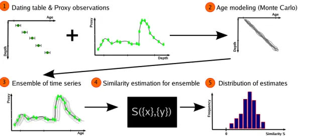
(Def. 4), visualized as step 1 in Fig. 3. The smoothing resulting from the size of the

25

(17)

CPD

9, 5299–5346, 2013

Title Page

Tables Figures

◭ ◮

Back Close

Full Screen / Esc

Discussion

P

a

per

|

Dis

cussion

P

a

per

|

Discussion

P

a

per

|

Discussio

n

P

a

per

|

samples in depth direction,σ_D, is assumed to be negligible here. The input proxy mea-surements are mapped to observation times in theage modeling process (def. 5). In general, algorithms to assess similarity between time series are not capable of pro-cessing probability distributions or confidence intervals instead of singleton values, neither for the observation times nor for the measurement values.

5

For Pearson correlation, an analytical approach to propagate the uncertainty around the input data into the correlation estimate is possible. However, Pearson correlation alone is insufficient to characterize similarity between paleoclimate time series in gen-eral and in the context of paleoclimate networks. Therefore a Monte-Carlo based ap-proach based on time series ensembles which are obtained via age modeling is used

10

here, to keep the flexibility regarding similarity estimators.

The task (assessing the uncertainty on the output statistic due to the input uncer-tainty) can be split into three parts:

– Drawing time series from the permitted ensemble of sample ages and corre-sponding observations (Monte Carlo Simulation, Fig. 3 step 3), then

15

– analyzing these samples individually, as if they had no age uncertainty (different similarity estimators), step 4 in Fig. 3,

– and finally assessing the distributions of the output values (i.e. the similarity), step 5 in Fig. 3.

Algorithmically, the approach can be described as

20

1. In a first step the input datasetsX andY are processed. The monotonicity of the control variables,d andD is checked. If it is not given, in an additional step the dataset is corrected/modified.

2. A Monte-Carlo simulation for the uncertain age estimates in the dating table is performed:Nens ages are drawn fromT

X

i ±σT_iX andT Y

j ±σT_jY, respectively, for all

25

(18)

CPD

9, 5299–5346, 2013

Title Page

Tables Figures

◭ ◮

Back Close

Full Screen / Esc

Discussion

P

a

per

|

Dis

cussion

P

a

per

|

Discussion

P

a

per

|

Discussio

n

P

a

per

|

in the dating table. This results in dating matrices ˆX and ˆY with Nens columns

containing the sampled ages. If no distribution of ages is otherwise given the ages are expected to be Gaussian distributed with the given standard deviation.

3. The age estimates in each column and ˆX( ˆY) are interpolated to the depths of the proxy observations:T=interp(D, ˆX,d) which results in a matrix, or an

ensem-5

ble, of reconstruction observation timesT. Together with the depthsd,Tforms an ensemble of possible age-depth relationships{T,d_}and with the proxy observa-tionsx it gives an ensemble of proxy time series_{T,x_}.

4. Each of the members of the ensemble of proxy time series is used as an input to the similarity statisticS(X,Y). This results in a distribution of estimatesp(S( ˆX, ˆY)).

10

5. Analysis of distribution S( ˆX, ˆY): Apart from inspection of mean, variance and skewness of this distribution, a hypothesis test can be conducted, comparing

S( ˆX, ˆY) with a distribution obtained from suitable surrogate time seriesS( ˆX∗, ˆY∗).

This approach is general in the sense that it is independent of the specific function

F([ ˆX, ˆY]) that maps the uncertain input to some output estimate. Apart from _F=S,_F

15

may represent any bivariate statistic, and with minor modification is also applicable to calculate the influence of sampling uncertainty on univariate statistics, like the auto-correlation coefficients or persistence times (Rehfeld et al., 2011; Mudelsee, 2002). Bi-variate similarity assessment is often concerned with estimation of a potentialcoupling strength S(ℓ) (hinting towards the same process of origin) and/or the lag of coupling

20

ℓ for model-building. For Pearson correlation, the ratio of shared vs. total variance be-tween two linearly correlated processes at a given lagℓ,S(ℓ) is given in the maximum of the cross-correlation function. While the relation to the overall variance of the pro-cesses does not necessarily hold by definition for other similarity measures, they, too, will observe the maximum of their similarity function max( ˆS), at the lag of couplingℓ.

25

(19)

CPD

9, 5299–5346, 2013

Title Page

Tables Figures

◭ ◮

Back Close

Full Screen / Esc

Discussion

P

a

per

|

Dis

cussion

P

a

per

|

Discussion

P

a

per

|

Discussio

n

P

a

per

|

2.3.1 Synthetic data

“True” growth histories for two synthetic stalagmites SS1 and SS2 and according cli-mate histories are obtained via simulation. These pseudo-archives are then “dated”, and correlated pseudo-proxy for the climate histories are “sampled”. Then the age modeling procedure is performed and its output is fed into similarity estimation. Finally,

5

we assess how much of the similarity that was originally present in the climate his-tory is still recognizable significantly, considering the uncertainties. The test strategy is illustrated in Fig. 3.

2.3.2 The synthetic stalagmite

A synthetic (or: virtual) stalagmite is grown for the sensitivity analysis. The main

pa-10

rameters controlled are

– the growth rateλin mm yr−1,

– the total length of the stalagmite (in mm),

– the type of accumulation (linear growth, or growth modeled via randomly dis-tributed accumulation rates).

15

A growth rate ofµ(λ(z))=1 mm yr−1 is chosen. Linear growth may be a reasonable first order approximation (Telford et al., 2004), but microscopically, the growth rates of natural archives archive vary. Therefore, γ(α, µ(λ(z))/α)-distributed accumulation times are drawn for each depthz_i={0, . . ., Z_}mm of the stalagmite, with the mean

µ(λ(z)) determined by the desired growth rate. Please refer to Rehfeld et al. (2011) for

20

a discussion of the gamma distribution for benchmark tests in paleoclimate time series analysis context, the role of parametersαandβand how they can be used to simulate increasing irregularity. The cumulative sum of the accumulation times then give the

“true” ages of the archive at the depthszi:ttruei (zi)= i P j=1

λi.

(20)

CPD

9, 5299–5346, 2013

Title Page

Tables Figures

◭ ◮

Back Close

Full Screen / Esc

Discussion

P

a

per

|

Dis

cussion

P

a

per

|

Discussion

P

a

per

|

Discussio

n

P

a

per

|

2.3.3 The simulated climate history

As in nature, each synthetic stalagmite SS1 and SS2 is attached to a climate history. The climate/pseudo-proxy simulation is based on the assumption that SS1 lies in an area whose climate is controlling that around SS2. We simulate climate variability us-ing two different coupling schemes, one linear, one nonlinear, to investigate how the

5

proposed methods perform.

Linearly coupled AR(1) processes

Assuming that the archive SS2 samples the same climate variability as SS1, in the same way though at a later time, we model such a causal sequence using coupled AR(1) processes. Then, thetrue proxy history of climate as recorded in SS1 is given

10

by

X ttrue_i ,z_i

=φXt_itrue −1

+σ_εε_i, (15)

and it determines part of the proxy history of SS2:

Y t_itrue,zi

=αXt_itrue₋_ℓ+σξξi. (16)

Here, ε and ξ are additional Gaussian white noise whose variances σ_ε and σ_ξ are

15

scaled such that the variances ofX andY are equal to unity (see Rehfeld et al., 2011, for more details),α is the coupling strength between SS1 and SS2 andφthe autocor-relation of SS1. Since there is no autocorrelative term inY_tthe expected similarityS(X,

Y) is equal to the cross correlation:S(X,Y)=ρ_xy=α.

Nonlinear threshold–AR(1) processes

20

Assume that SS1 samples climate variability in a certain place, and this can be mod-eled as in Eq. (15). Then the climate variability in another place, where SS2 is located,

(21)

CPD

9, 5299–5346, 2013

Title Page

Tables Figures

◭ ◮

Back Close

Full Screen / Esc

Discussion

P

a

per

|

Dis

cussion

P

a

per

|

Discussion

P

a

per

|

Discussio

n

P

a

per

|

could be controlled in a nonlinear manner: In principle, the processes are negatively correlated, similar to Eq. (16). If, however, a threshold in the climate system is ex-ceeded, X(t)> τ, the correlation changes and might even become positive. Such a multi-scale behavior can be modeled using Threshold-AR-processes (TAR, Tsay, 1989), which are similar to the regime-dependent AR models Zwiers and Storch (1990)

5

used to model the behavior of the Southern Oscillation. Assume that the negative cou-plingα below the thresholdτ=0, for X(t₋1)6τ _{turns into a positive correlation, with}

the same magnitude, forX(t−1)> τ. Then the proxy history of SS2 can be modeled as

Y t_itrue,zi

=α·κ ttrue

Xttrue_i₋_ℓ +σ ttrue

ξi, (17)

10

where theκ=−1 ifX(t−1)6τandκ=1 whenX(t−1)> τ. In both cases the variance

of the innovation termξis scaled such that the overall variance ofY is equal to unity.

2.3.4 “Dating” of the synthetic stalagmite

Mimicking the real life situation, the true growth history of the synthetic stalagmite,

z(ttrue) is, in the following, inaccessible. The stalagmite is subjected todatingalong its

15

depth. The dating table contains the for the dating depthsD, the estimated age at these depths,T_j, the proxy measurement sample widthσ_Dand the age uncertaintyσ_T.

In real life, the stalagmite would be dated using radiometric dating techniques based on Uranium-Thorium (Sinha et al., 2007; Dykoski et al., 2005; Breitenbach et al., 2012) or radiocarbon (Yadava et al., 2004; Webster et al., 2007), yielding an estimate ofT(z_j)

20

at a few points. The corresponding dating uncertainty, in reality dependent on many factors from initial isotope concentrations, overall age of the core, dating technique to lab and contamination (Fairchild and Baker, 2012), often lies between 0.1 to 0.5 % of the age.

For the synthetic stalagmites, dating “samples” are taken at equidistant depths D_j 25

and the center points of the assumed age distribution are taken directly from thetrue

(22)

CPD

9, 5299–5346, 2013

Title Page

Tables Figures

◭ ◮

Back Close

Full Screen / Esc

Discussion

P

a

per

|

Dis

cussion

P

a

per

|

Discussion

P

a

per

|

Discussio

n

P

a

per

|

age-depth relationship. The age uncertainty, however, is modeled as increasing pro-portionally with age, asp·T_j.p thus denotes the (im-)precision of the dating and is varied in the following numerical experiments.

2.3.5 Age modeling

Age modeling aims at reconstructing the “true” depth-age relationship that is

inacces-5

sible in real paleoclimate archives.

Based on the synthetic stalagmite dating tables Dx and Dy for SS1 and SS2, the “observation times” for the proxy observationsXd and Yd,tx andty, are constructed by interpolation from the known ages (see Eq. 13). In Monte-Carlo based numerical frameworks such as StalAge (Scholz and Hoffmann, 2011) or COPRA (Breitenbach

10

et al., 2012), an ensemble of age modelsT={t_k,z_k}k=1,...,Nens _{is created, which, in their} entirety, reflect the age uncertainty of the estimated depth-age relationship. Based on this ensemble of age models, the uncertainty in the similarity estimates can be inferred, as is visible in Fig. 3.

In summary, the test plan is thus as follows:

15

1. Simulate a growth historyz(t) of a synthetic stalagmite of length Z mm, corre-sponding to a “true” age–depth relationship t_itrue(z_i), resp. z_i(ttrue). For this, as-sume gamma-distributed growth and an accumulation rateλ=1 mm yr−1.Z can be varied to study the influence of changing time series length.

2. Simulate proxy histories_{T,x_}SS1and_{T,y_}SS2according to thetrue growth

his-20

tory using coupled autoregressive processes (cf. Eqs. 16 and 17). Forget the true growth history.

3. Sample the true growth history at the dating depths and infer corresponding un-certainties.

4. CreateNens surrogate dating tables for SS1 and SS2 with increasing uncertainty

25

(23)

CPD

9, 5299–5346, 2013

Title Page

Tables Figures

◭ ◮

Back Close

Full Screen / Esc

Discussion

P

a

per

|

Dis

cussion

P

a

per

|

Discussion

P

a

per

|

Discussio

n

P

a

per

|

5. Assess if the estimatesS_{( ˆ}_{X, ˆ}_{Y) are statistically significant for the given uncertainty,} and how they are influenced by sampling heterogeneity and time uncertainty.

The core of the COPRA algorithm is used for MC simulations.Nens=2000 MC iterations

are used to sample the probability space and linear interpolation is employed to infer ages between point estimates of the age at depth.

5

3 Tests on synthetic stalagmites

We evaluate the performance of the different estimators described in Sect. 2, for which parameter choices and references are given in Table 1.

3.1 Characterization of linear proxy dependency

We first consider the linear dependency case, where the proxy history of SS1 is

lin-10

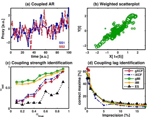
early correlated with that of SS2 a lag time ℓ later. We chose a length for the sta-lagmite of L=100 mm for which we expect the time series to be roughly 100 yr long (cf. Sect. 2.3.2) and linearly correlated, as in Fig. 4a. For each test 100 time series were generated from AR1 processes (cf. Sect. 2.3.3), where processY is coupled to process X at an intrinsic lag ℓ and with a coupling strength α. The autocorrelation

15

parameter was set to φ=0.8, the coupling lag to ℓ=5 and the coupling parameter toα=0.6. For such stochastic processes, the true similarity function is single-peaked, with its peak height determined byα, and its location on the lag-axis by the coupling lag

ℓ. The time series are irregular, therefore a direct scatterplot of the data is not possible. Figure 4b shows a weighted scatterplot where the time series have been reconstructed

20

using Gaussian weights, as for the MI estimation in Sect. 2.2.2.

The tests were guided by two questions: Do the similarity estimators reflect the actual similarity (here: the coupling strength at lag ℓ,α) truthfully and monotonically? And, how well do they identify the lag of couplingℓas the maximum of the similarity function?

(24)

CPD

9, 5299–5346, 2013

Title Page

Tables Figures

◭ ◮

Back Close

Full Screen / Esc

Discussion

P

a

per

|

Dis

cussion

P

a

per

|

Discussion

P

a

per

|

Discussio

n

P

a

per

|

To answer the first question we fix the imprecision at zero (at the dating points) and vary the coupling strength by setting the parameterα in Eq. (16) to values from 0.1 to 1. The results are given in Fig. 4c. The expected value of the similarity,αest, and

the variance of the estimate are computed from the mean and standard deviations of the estimated αest,i for 100 realizations for each value of the coupling parameter.

5

Each of the similarity measures returns estimates whose expectation values increase monotonically with the actual similarity,αtruein Eq. (16), except for the ESF, which has

a single reversal which may be due to the low number of MC realizations (100) for each point in this diagram.

In practical data analysis, the potential lag and strength of (primary) coupling,

iden-10

tified as the maximum of the similarity function is of interest (e.g. for model-building). If no age uncertainty exists at the dating points, the maximum of the similarity function correctly identified in 50–60 % of the ensemble cases. When time-scale uncertainty exists in the time series, this becomes di_fficult quickly (Fig. 4d). When the percentage has dropped to _n1

ℓ ≈0.05, where nℓ is the number of lags for which S(ℓ) has been 15

estimated, the maxima of the similarity functions are perfectly uncorrelated. This limit is approached as an imprecision of more than 10 % is reached. Increasing imprecision contained in the time series also results in increasing estimation error (i.e. RMSE, root mean square error) for the similarity at the lag of coupling,S(ℓ) (results not shown). When the stalagmite length is increased the time series length increases and both the

20

RMSE and the false identification rate decrease for all estimators.

3.2 Nonlinear dependencies

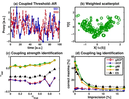
For the nonlinear TAR model, the time series in Fig. 5a are not straightforward to com-pare visually as the linearly coupled ones in Fig. 4a. The weighted scatterplot for these time series in Fig. 5b shows the two different slopes of the positive and negative

corre-25

lation regimes above and below the threshold value of zero.

The comparison of true vs. estimated coupling strength α in Fig. 5c shows no monotonous behavior for the linear correlation measures and no overall increase of

(25)

CPD

9, 5299–5346, 2013

Title Page

Tables Figures

◭ ◮

Back Close

Full Screen / Esc

Discussion

P

a

per

|

Dis

cussion

P

a

per

|

Discussion

P

a

per

|

Discussio

n

P

a

per

|

their expected similarity estimates with the coupling strength. The MI estimators retain a monotonic increase, starting from a considerable bias value, while the ESF increases monotonically, but does not show consistent similarity estimate increases until the cou-pling strength is rather large. The monotonicity and linearity of the response for gMI, iMI and ESF improve considerably when the time series are chosen longer, i.e. with a

5

length of 200 or more (results not shown).

In the identification of the maximum lag the Gaussian MI succeeds most often for im-precisions up to 2.5 %. For more imprecise datasets the ESF remains stable, while the other measures perform worse and worse. The linear estimators, gXCF and iXCF do not identify the maxima correctly, neither the coupling strength, nor the lag of coupling.

10

3.3 Error source attribution

Age uncertainty has a considerable impact on the accuracy of similarity estimates, as we have shown in the previous section. But to what extent can this impact be attributed to short length of the time series, or the time series irregularity that results from the increasing age uncertainty? The uncertainty around the ages in the dating table is,

15

in Monte-Carlo-based age-depth modeling, reflected by drawing different “dates” from distributions around these ages for each MC realization. These realizations will there-fore have different partial slopes between any dateD_i and D_i₊₁. This corresponds to different estimated growth rates for the individual segments of the synthetic core. At a proxy sampling rate over depth that is constant, this will lead to uneven observation

20

times for the time series which correspond to the MC realizations, and this irregularity increases with the age uncertainty. The RMSE of S(ℓ) is, however, also dependent on the irregularity of the time series, as it was shown for both XCF and MI previously (Rehfeld et al., 2011, 2013).

To separate these sources of uncertainty,M=2000 realizations of coupled climate

25

histories, as defined in Sect. 2.3.2, were generated in three different ways: age un-certain,irregularly and regularly sampled. The age uncertain ensembles were the di-rect product of the age modeling e_fforts, as in the previous sections and with same

(26)

CPD

9, 5299–5346, 2013

Title Page

Tables Figures

◭ ◮

Back Close

Full Screen / Esc

Discussion

P

a

per

|

Dis

cussion

P

a

per

|

Discussion

P

a

per

|

Discussio

n

P

a

per

|

parameter settings (φ=0.8, α=0.9, ℓ=5). For the irregular dataset the proxy histo-ries were re-generated with the true coupling strength on the irregular timescales of the age modeling output. To assess the impact of regular sampling, regular time se-ries of the same length, average temporal spacing and coupling scheme were also simulated. We evaluated the performance of the di_fferent estimators for the di_fferent

5

sampling schemes at increasing dating imprecision using theroot mean square error

(RMSE) of the estimators for the target coupling parameterα:

RMSE (αest) = q

var (αest)+bias (αest)2, (18)

where bias(αest)=αtrue−αest.

We did this separately for each sampling scheme to obtain the RMSEreg, the

10

“baseline” RMSE for each estimator under regular sampling, RMSE_irreg for the irreg-ularly sampled ensembles and the RMSEau for the age uncertain ensemble. Coupling

strength, autocorrelation and time series length were fixed to the same values for the three different sampling schemes. To improve the comparability for the MI estimators the bias offset was estimated from uncorrelated time series with the same

autocorrela-15

tion and length and subtracted prior to the conversion to the XCF scale.

Based on the assumption that the RMSE should increase from regular to irregular to age uncertain time series,

RMSE_reg <RMSE_irreg <RMSE_au,

the “baseline” contribution is estimated from regular time series as RMSEreg, the

ad-20

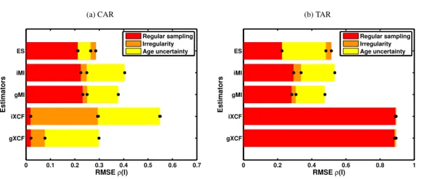
ditional contribution from time scale irregularity as RMSE_irreg₋RMSE_reg and the addi-tional RMSE of the age uncertain time series’ similarity as RMSEageunc−RMSEirreg.

The results, averaged over the realistic imprecision values (the 2nd–5fth points in Figs. 4d and 5d), are given in Fig. 6.

Ideally the RMSE should of course be as small as possible. For the linear (CAR)

25