Comparison of three methods for the estimation of cross-shock electric potential using Cluster data

(1)

www.ann-geophys.net/29/815/2011/ doi:10.5194/angeo-29-815-2011

Annales

Geophysicae

Comparison of three methods for the estimation of cross-shock

electric potential using Cluster data

A. P. Dimmock1, M. A. Balikhin1, and Y. Hobara2

1_{Automatic Control & Systems Engineering, University of Sheffield, Sheffield, UK}

2_{Department of Communication Engineering and Informatics, The University of Electro-Communications, Tokyo, Japan}

Received: 28 February 2011 – Revised: 15 April 2011 – Accepted: 18 April 2011 – Published: 13 May 2011

Abstract. Cluster four point measurements provide a com-prehensive dataset for the separation of temporal and spa-tial variations, which is crucial for the calculation of the cross shock electrostatic potential using electric field mea-surements. While Cluster is probably the most suited among present and past spacecraft missions to provide such a sep-aration at the terrestrial bow shock, it is far from ideal for a study of the cross shock potential, since only 2 components of the electric field are measured in the spacecraft spin plane. The present paper is devoted to the comparison of 3 differ-ent techniques that can be used to estimate the potdiffer-ential with this limitation. The first technique is the estimate taking only into account the projection of the measured components onto the shock normal. The second uses the ideal MHD condition

E_·B₌0 to estimate the third electric field component. The last method is based on the structure of the electric field in the Normal Incidence Frame (NIF) for which only the po-tential component along the shock normal and the motional electric field exist. All 3 approaches are used to estimate the potential for a single crossing of the terrestrial bow shock that took place on the 31 March 2001. Surprisingly all three methods lead to the same order of magnitude for the cross shock potential. It is argued that the third method must lead to more reliable results. The effect of the shock normal inac-curacy is investigated for this particular shock crossing. The resulting electrostatic potential appears too high in compari-son with the theoretical results for low Mach number shocks. This shows the variability of the potential, interpreted in the frame of the non-stationary shock model.

Keywords. Space plasma physics (Electrostatic structures; Shock waves)

Correspondence to: A. P. Dimmock

(a.dimmock@sheffield.ac.uk)

1 Introduction

(2)

ultra-relativistic shocks associated with gamma ray burst af-terglow indicate such shocks are formed by filamentational instability as in classical anomalous process based shock models.

However, as mentioned above for the quasi-perpendicular planetary and interplanetary shocks that are observed in the solar system, macro electric and magnetic fields in the shock front can explain the energy redistribution without invoking models based on instabilities (Wu, 1984; Leroy and Man-geney, 1984; Scudder et al., 1986; Balikhin and Gedalin, 1994). Therefore comprehensive measurements of electro-static potential and the magnetic field structure of the shock front are required to understand the evolution of the plasma parameters across these shocks. The number of studies de-voted to the magnetic field structure of the terrestrial bow shock significantly outnumber the studies of the electric field. One of the possible reasons is due to the complexity of the electric field measurements across the region with nonuni-form plasma temperature/density. Only a few papers de-voted to the electric field and electrostatic potential in the shock have been published (Heppner et al., 1978; Wygant et al., 1987; Formisano, 1982; Scudder et al., 1986; Balikhin et al., 2002; Scholer et al., 2003) in comparison to hun-dreds dedicated to the magnetic field structure of the various types of shocks. The estimate of the cross shock potential is also susceptible to the inaccuracy of the calculated rela-tive shock/spacecraft velocity, because it requires the spacial integration of the electric field over the spatial coordinates. Therefore, the ability to distinguish between temporal and spatial variations is crucial for the reliable identification of the shock front potential. Four closely spaced satellites such as Cluster appear ideal for the analysis of the shock poten-tial. However, the electric field instrument onboard each of the Cluster satellites does not measure all three components of the electric field, providing only the X- and Y-components in the satellite spin plane. In order to exploit the spatio-temporal potential of the Cluster mission, additional assump-tions are required to estimate the potential in such cases. A straight-forward approach which involves no computation prior to the calculation of the potential assumes that if the angle between the spin plane and the shock normal is small, then the potential can be estimated using only the two avail-able electric field components. If the spin plane is not almost perpendicular to the shock normal such an estimate should give a correct order of magnitude for the cross shock poten-tial. The second method that has been used is based on the assumptionE_·B₌0 (ideal MHD). This condition allows the identification of the third component of the electric field and subsequently the cross shock potential. This methodology has been used in a number of studies (Bale and Mozer, 2007; Bale et al., 2008). The final method to be considered in the present study uses the structure of electric field in the Nor-mal Incidence Frame (NIF) in which the upstream velocity lies along the shock normal. Only two components of elec-tric field exist in this frame: the potential along the shock

normal, andV_×B. As velocity is directed along the normal, only the component of the magnetic field that is perpendicu-lar to the shock normalBperpcontributes to the termV×B.

ThereforeE_·_B_perp_{must be equal to zero, giving the}

possibil-ity to determine the missing third component of the electric field and therefore identify the cross-shock potential. The present paper is devoted to the comparative study of these 3 methods applied to a particular shock observed by the four Cluster spacecraft on 31 March 2001.

2 Data and instrumentation

The data used in this study were collected by the Clus-ter spacecraft during a day of 11 bow shock crossings on 31 March 2001. The electric field measurements were made by the Electric Fields and Waves experiment (EFW) (Gustafsson et al., 1997), which is part of the wave con-sortium controlled by the Digital Wave Processor (DWP) (Woolliscroft et al., 1997). The EFW instrument consists of 4 spherical probes deployed on 44 m wire booms (88 m sen-sor separation), the potential difference between the probes is used to measure the electric field components in the spin plane of the spacecraft (ISR2). In the ISR2 frame, the spacecraft spin axis is represented by the X-axis. When the ISR2 frame is inverted about the spin axis it varies by

<6◦of the geocentric solar ecliptic (GSE) frame. A signi-ficant limitation of this instrument is the absence of a third field vector, as a result only 2 components are recorded in the ISR2 frame. The Fluxgate Magnetometer (FGM) in-strument (Balogh et al., 1997) provides magnetic field mea-surements which are used to identify the shock crossing re-gion, and correlate with the EFW datasets. The time reso-lution of the EFW and FGM datasets are 25 Hz and 22 Hz respectively. Ion density (Ni) used to calculate Alfv´en

Mach number(Ma), was estimated using the electron plasma

frequency ωpe measured by the WHISPER instrument

(D´ecr´eau et al., 1997). The solar wind upstream bulk flow velocity Vup

was obtained from the Cluster Ion Spectro-meter (CIS) instrument (R`eme et al., 1997).

3 Shock crossing: 31 March 2001, 18:28 UT

The present paper is devoted to a particular shock that oc-curred on 31 March 2001 at 18:28 UT. On this day solar wind conditions were to some extent irregular due to the passage of a CME. The magnetic field and solar wind velocity up-stream of the shock measured by the Cluster 1 spacecraft were 27 nT and 590 km s−1, respectively. The model normal (Farris et al., 1991) in the GSE frame is [0.92,−0.09, 0.37], and the shock velocity was determined to be 29 km s−1. Re-maining parameters areθBN=88◦and plasma densityNi=

(3)

0 5 10 15 20 25 30 0

50 100 150

|B| (nT)

Time in seconds since ï 18:28:00

Shock crossing observed by all 4 Cluster spacecraft on 31 March 2001

Cluster 1 Cluster 2 Cluster 3 Cluster 4

0 10 20 30 0 10 20

0 50 100

Ex

(mV m

ï

1)

Time in seconds past ï 18:28:00 Cluster 1

0 10 20 30 0 10 20

0 50 100

Ex

(mV m

ï

1)

0 10 20 30 0 10 20

0 50 100

Ex

(mV m

ï

1)

0 10 20 30 0 10 20

0 50 100

Ex

(mV m

ï

1)

Fig. 1. Measurements made by the four Cluster spacecraft as they observed one of eleven bow shock crossing on 31 March 2001 at 18:28 UT.

The top panel illustrates the magnitude of the magnetic field profile measured by the four FGM instruments onboard each spacecraft. The four lower panels show the electric field measurements recorded by the relative EFW instruments over the same time period.

10 20 30 40 50 60 70 80 90 100 110

|B| (nT)

Shock crossing observed by Cluster 1 on 31 March 2001

0 5 10 15 20 25

ï20 0 20 40 60 80 100

Ex

(mV m

ï

1)

Time in seconds past ï 18:28:00

Fig. 2. A shock crossing observed by the Cluster 1 spacecraft at 18:28 on 31 March 2001. The upper panel shows the magnitude of the

magnetic field profile measured the Cluster 1 FGM instrument across the shock. The lower panel shows the x-component of the electric field recorded by the EFW instrument over the same time interval (in the spacecraft spin frame).

The sequence in which the Cluster spacecraft encountered the bow shock was C4, C2, C1 and finally C3. This is illus-trated by the top panel of Fig. 1. Additionally Fig. 2 shows the measurements during the shock crossing recorded by the FGM and EFW instruments onboard the Cluster 1 space-craft. The top panel of Fig. 2 displays the magnitude of the magnetic field several seconds before and after the shock. The magnetic profile displays an abundance of low frequency plasma waves prior to the shock crossing which commence at

approximately 18:28:07 UT. The lower panel illustrates the X-component of the EFW measurements in the spacecraft spin frame. The electric field appears constant upstream of the shock at around 5 mV m−1which reflects theV_×B_term.

(4)

0 5 10 15 20 25 30 35 40 45

ï40

ï20 0 20 40 60 80 100

|B| (nT)

Shock crossing observed by the Cluster 1 and 4 spacecraft on 31 March 2001

ï5 0 5 10 15 20 25 30 35 40

ï40

ï20 0 20 40 60 80 100

|B| (nT)

|B| Bn

Cluster 4 Cluster 1

Fig. 3. The magnetic field profile of a shock crossing observed by the Cluster 1 and 4 satellites on 31 March 2001. The time interval shows

the crossing several seconds upstream and around 30 s downstream of the crossing. The black line shows the magnitude of the magnetic field whereas the grey line is the magnetic field projected along the normal. The upper and lower panels represent the Cluster 1 and Cluster 4 spacecraft, respectively.

of the terrestrial bow shock and have been statistically stud-ied by Walker et al. (2004). The lower panels of Fig. 1 demonstrate that a small scale structure within the shock front, has been observed in the electric field by all four Clus-ter spacecraft.

4 Shock normal

The shock normaln_ˆ _{is one of the key parameters in the}

esti-mate of the cross-shock potentialφ. This is not only because it is the electric field component parallel ton_ˆ ₍_E_n_{) that}

con-tributes toφ, but also due to the effect of the normal shock-spacecraft velocity on the spatial integration of the electric field. In the present paper the shock normalnhas been iden-tified using the Farris et al. (1991) model shock surface. The multi spacecraft timing analysis (Schwartz, 1998) produces a normal that has a very small angle (<5◦_{) with} _n_ˆ_.

Fig-ure 3 displays|B|and the projection of the magnetic field alongn_ˆ ₍_B_n_{), for the Cluster 1 (top) and Cluster 4 (bottom)}

spacecraft. It can be seen that the average values ofBn do

not possess any significant change within the ramp where

|B|experiences a 60–70 nT change. The change of the av-erage value from the far upstream to the deep downstream is also insignificant, supporting the estimate of the normal

ˆ

n_{. Spacecraft 2 and 3 show similar results. However, for all}

four spacecraft the decreasing portions of overshot coincide with deviation inBn as also can be seen in Fig. 3. This can

be explained by a presence of an additional ripple-like local structure.

The velocity along the shock normal was determined based on a selection of the 6 possible geometric parings of the 4 Cluster satellites as they encountered the bow shock. Only 3 pairs of crossings have been used, since the other 3 separation vectors were close to being perpendicular to

ˆ

n_{. The following 3 spacecraft pairings were used, C1}_→_C4,

C2→C3 and C3→C4. The total variation between the 3 identified velocities was less that 15 %. The mean of the 3 velocity pairings 29.4 km s−1has been used as the shock ve-locityVs.

5 Methodology for the estimation of cross-shock potential

As the electric field is frame dependent, the Lorentz transfor-mation should be used to estimate the cross shock potential in the NIF frame using the electric field data measured in the spacecraft frame. The electric field components resulting fromVsandVnif(NIF frame velocityVnif=nˆ× Vu×nˆ)

could reach quite significant values of a few mV m−1which may contribute errors leading to the miscalculation ofφ.

Electric field measurements made by the EFW instrument onboard all 4 Cluster spacecraft consist of only 2 components directed along the X and Y directions in the spacecraft spin frame. As a result only an estimate ofφcan be calculated. The present paper is devoted to three separate techniques for estimating cross shock potential.

The estimate of the cross shock potentialφestcan be

(5)

0 5 10 15 20 25 0

20 40 60 80 100 120 140 160

|B| (nT)

q

(V / 20, / 100E

i

up

)

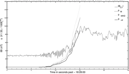
Three estimates of the crossïshock electric potential for a shock observed by Cluster 1 on 31 March 2001

|B

C1|

q_M

q_MHD

q_nif

Fig. 4. A shock crossing made by the Cluster 1 spacecraft around 18:28 on 31 March 2001. The grey line shows the magnetic field magnitude

measured by the Cluster 1 FGM instrument during the bow shock crossing. The dotted black line is the estimate based on the assumption that the electric field alongB_{is zero. The black dashed line shown the estimate based on only the 2 measured electric field components. The black}

solid line represents the potential estimate by evaluating the missing electric field component based on the NIF condition (ENIF·B⊥=0).

this procedure is that the direction of the shock normal is not almost perpendicular to the axis of the spacecraft spin plane. Such an estimate will provide a correct spatial scale of the cross shock potential and a reasonable estimate of its magni-tude. However, this method cannot be expected to produce a precise magnitude of the potential|φ|.

To obtain more reliable and accurate values of the cross shock potential from Cluster data, the properties of the elec-tric field in the NIF frameENIFof reference can be used. In

the NIF the motional componentV_u_×B_{is perpendicular to}

the electrostatic component which is the gradient ofφalong the normal. The upstream magnetic field can be decomposed into the component parallel ton_ˆ ₍_B_n_{), and a perpendicular}

componentB⊥. The conditionENIF·B⊥=0 allows the

de-termination of the third unmeasured component of the elec-tric field.

Often when only two components of the electric field are available the third component is reconstructed by assuming that the component ofE _alongB _{is zero (Bale and Mozer,}

2007)E_·B₌_{0 (ideal MHD). It is worth noting that whilst}

this approximation might provide an accurate estimate for some other structures and regions, it is unacceptable for the terrestrial bow shock. This can be illustrated by electron dy-namics. The de-Hoffman-Teller frame (HTF) of reference is defined by the condition that the upstream velocity is parallel to the upstream magnetic field. Therefore the motional com-ponent of electric field vanishes, leading to charged particle energy conservation in the HTF. As discussed by Goodrich and Scudder (1984) the electrostatic potential in the HTF is directly related to the electron energization. Setting the par-allel electric field to zero will distort the value of the

electro-static potential in HTF for quasi-perpendicular shocks. As a result the “bump on flattop” electron distributions (Feldman et al., 1983) would not be observed. In spite of all this crit-icism of the E_·B₌_{0 assumption, it will be used in the}

present paper for comparison with the results obtained by the first two methods.

It is worth noting that upstream of the shock front the only component that contributes to the DC electric field is the mo-tional V_×B _{field. This value will be constant across the}

shock. Therefore, the upstream value ofV_×B _{can be used}

to account for the motional electric field across the whole shock front.

Finally to calculate the electrostatic potential,ENIFis

spa-tially integrated through the shock front, including both the foot and shock ramp regions. The integration is discontinued at the end of the shock ramp just prior to downstream.

6 Results

The change of the electrostatic potential within the shock crossing measured by the Cluster 1 spacecraft, is displayed in Fig. 4, together with the magnitude of the magnetic field (grey solid line). The zero level reference line ofφ=0 is also shown in this figure. Three methods of potential esti-mates lead to the differences in theφ. The lowest value of the potential is a result of the method based on the NIF con-ditionENIF·B⊥=0 (solid line). The highest is based on the

(6)

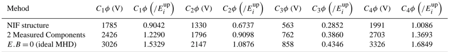
Table 1. Cross shock potential estimates for each electric field dataset. Provided are calculations for the potential in Volts and also the

potential normalised with respect to the upstream ion kinetic energy (Eup_i ).

Mehod C₁φ(V) C₁φ/E_iup C₂φ(V) C₂φ/E_iup C₃φ(V) C₃φ/E_iup C₄φ(V) C₄φ/E_iup

NIF structure 1785 0.9042 1330 0.6737 563 0.2852 1991 1.0086

2 Measured Components 2426 1.2290 1796 0.9098 762 0.3860 2703 1.3693

E.B=0 (ideal MHD) 3026 1.5329 2147 1.0876 858 0.4346 3326 1.6849

1 2 3 4

0 0.5 1 1.5 2 2.5 3

Limits for q ± 5o variation of normal components

Cluster Spacecraft #

q

/ E

i

up

q_MHD q_M q_NIF

Fig. 5. Electric cross-shock potential estimates of all four

Clus-ter spacecraft. The circle markers represent the potential estimates prior to any variation whereas, the error bars represent the upper and lower limits of the maximum and minimum potential evaluations as a result of a variation about the model normal of±5◦.

Volts and the upstream ion energyE_iup=miV

2 up

2 . Table 1

sum-marises the values of the overall cross shock potential change obtained by these 3 techniques for all four Cluster spacecraft. It can be seen that the relative values of the potential estimate by all 3 methods are similar to these obtained by the Clus-ter 1 spacecraft. The lowest and highest values are always resulting fromENIF·B⊥=0 andE·B=0, respectively. The

2 component based estimate values are always intermediate with respect to the other methods. Even the lowest of the potential estimates obtained using NIF condition appear too high in the case of the Cluster 1 and 4 crossings. The possible physical reasons for such high values of the potential will be explained later in the Discussion section. To ensure that these values are not the result of an error during the identification of the shock normal and consequent shock velocity, the ef-fect of the normal variation has been investigated for the NIF condition based method. The direction of the normaln_ˆ has been subjected to a variation of a 10◦cone around its iden-tified model value. Obviously any variation in the direction of the normal leads to variation in the shock velocity, NIF frame,ENIFetc. The extreme minimal and maximum values

resulting from such a variation within the cone are shown as the upper and lower boundaries for the error bars in Fig. 5. It can be seen that even minimal values of the potential for

Cluster 4 resulting from such variation is quite high at about 80 % of the upstream ion kinetic energy.

7 Discussion

The change of the cross shock potential for Cluster 1 dis-played in Fig. 4 is representative of the four spacecraft cross-ings of this shock. The increase in the potential starts up-stream of the ramp in the region of low frequency turbulence. Since ISEE and AMPTE projects, it is known that this region almost coincides with the foot of a quasi-perpendicular shock (e.g. Krasnoselskikh et al., 1991). Initially it was thought that these waves are the result of plasma instabilities caused by the counter streaming plasma flow and the beam of re-flected ions. However, data from closely spaced spacecraft (inside the coherency length of the turbulence) enabled the dismissal of these models and indicated that these waves are the result of the nonlinear evolution of the shock front itself (Krasnoselskikh, 1985; Balikhin et al., 1997, 1999; Walker et al., 2008). The increase of the potential in the foot is about a quarter of the overall change. The rest of the in-crease corresponds to the region of the magnetic ramp. A small scale structure is evident in the electric field at around 18:28:13.5 in Fig. 1 which contributes around 15 % of the electrostatic potential. According to the estimation based on the NIF condition, the contribution of this small scale struc-ture is around 300 V. Such a considerable increase of the po-tential over a small spatial scale should lead to non-adiabatic dynamics of electrons and a corresponding increase of tem-perature (Gedalin et al., 1995; Balikhin and Gedalin, 1994; Balikhin et al., 1998). The increase of the cross shock poten-tial should also lead to the decrease of the ion thermal energy downstream of the shock e.g. Ofman et al. (2009).

(7)

protons). Therefore the value of the upstream average ion kinetic energy based on the proton mass should lead to sig-nificant underestimation. The second reason is the unusual CME observed on this day. There are a total of 9 crossings of the terrestrial bow shock in a short period of about 2 and a half hours. This indicates non-stationarity of the solar wind conditions. Such non-stationarity can lead to shock reforma-tion induced by the change in the abnormal solar wind con-ditions, and results in unusual values of the potential for this particular crossing.

The main conclusion that should be drawn from this study is that all three methods lead to the same order of magni-tude of the cross shock potential, and exactly the same spa-tial scales of the potenspa-tial change. However as these methods still lead to a significant difference in the potential estimates, the NIF derived method should be used for a more accurate estimation. As theE_·B₌0 technique is based on an as-sumption that is not valid at the shock front. The simplistic methodology of the potential estimate when only two mea-sured components are taken into account (without any other additional assumptions) are able to provide the same relia-bility ofφspatial scales as the more sophisticated technique that uses the NIF conditionENIF·B⊥=0. The spatial scales

of the shock are one of the most important parameters, as they are related to the physical processes that balance non-linearity and lead to the shock structure formation (Kennel et al., 1985; Sagdeev, 1979; Papadopoulos, 1981). In ad-dition, the spatial scale determines the mechanism of inter-action between the incoming solar wind particles, and the macro electric and magnetic fields within the shock. While there are many studies of the magnetic field scales within the shock front (e.g. Balikhin et al., 1995; Hobara et al., 2010; Newbury and Russell, 1996), only a few studies are devoted to the scales of the electric field e.g. Walker et al. (2004). The results of the present study facilitate the ability to estimateφ

spatial scales in the case of limited electric field datasets such as Cluster, and can allow an easier comprehensive statistical study of these scales based on a large number of shocks ob-served by Cluster.

Acknowledgements. This work was supported by STFC and EP-SRC grants. The authors wish to acknowledge the Custer FGM, EFW, CIS, WHISPER and DWP teams for providing the datasets for this study.

Guest Editor M. Gedalin thanks L. Ofman and another anony-mous referee for their help in evaluating this paper.

References

Bale, S. D. and Mozer, F. S.: Measurement of Large Parallel and Perpendicular Electric Fields on Electron Spatial Scales in the Terrestrial Bow Shock, Phys. Rev. Lett., 98, 205001, doi:10.1103/PhysRevLett.98.205001, 2007.

Bale, S. D., Mozer, F. S., and Krasnoselskikh, V. V.: Direct mea-surement of the cross-shock electric potential at low plasmaβ, quasi-perpendicular bow shocks, ArXiv e-prints, 2008.

Balikhin, M. and Gedalin, M.: Kinematic mechanism of electron heating in shocks: Theory vs observations, Geophys. Res. Lett., 21, 841–844, doi:10.1029/94GL00371, 1994.

Balikhin, M., Krasnosselskikh, V., and Gedalin, M.: The scales in quasiperpendicular shocks, Adv. Space Res., 15, 247–260, doi:10.1016/0273-1177(94)00105-A, 1995.

Balikhin, M. A., Walker, S. N., de Wit, T. D., Alleyne, H. S. C. K., Woolliscroft, L. J. C., Mier-Jedrzejowicz, W. A. C., and Baumjo-hann, W.: Non-stationarity and low frequency turbulence at a quasiperpendicular shock front, Adv. Space Res., 20, 729–734, doi:10.1016/S0273-1177(97)00463-8, 1997.

Balikhin, M., Krasnoselskikh, V. V., Woolliscroft, L. J. C., and Gedalin, M.: A study of the dispersion of the electron distribu-tion in the presence of E and B gradients: Applicadistribu-tion to electron heating at quasi-perpendicular shocks, J. Geophys. Res., 103, 2029–2040, doi:10.1029/97JA02463, 1998.

Balikhin, M. A., Alleyne, H., Treumann, R. A., Nozdrachev, M. N., Walker, S. N., and Baumjohann, W.: The role of nonlinear in-teraction in the formation of LF whistler turbulence upstream of a quasi-perpendicular shock, J. Geophys. Res. (Space Physics), 104, 12525–12536, doi:10.1029/1998JA900102, 1999.

Balikhin, M. A., Nozdrachev, M., Dunlop, M., Krasnoselskikh, V., Walker, S. N., Alleyne, H. S. C. K., Formisano, V., An-dre, M., Balogh, A., Eriksson, A., and Yearby, K.: Obser-vation of the terrestrial bow shock in quasi-electrostatic sub-shock regime, J. Geophys. Res. (Space Physics), 107, 1155, doi:10.1029/2001JA000327, 2002.

Balikhin, M. A., Zhang, T. L., Gedalin, M., Ganushkina, N. Y., and Pope, S. A.: Venus Express observes a new type of shock with pure kinematic relaxation, Geophys. Res. Lett., 35, L01103, doi:10.1029/2007GL032495, 2008.

Balogh, A., Dunlop, M. W., Cowley, S. W. H., Southwood, D. J., Thomlinson, J. G., Glassmeier, K. H., Musmann, G., Lühr, H., Buchert, S., Acuña, M. H., Fairfield, D. H., Slavin, J. A., Riedler, W., Schwingenschuh, K., and Kivelson, M. G.: The Cluster mag-netic field investigation, Space Sci. Rev., 79, 65–91, 1997. Décréau, P. M. E., Fergeau, P., Kranoselskikh, V., Lévêque, M.,

Martin, P., Randriamboarison, O., Sen´e, F. X., Trotignon, J. G., Canu, P., and M¨ogensen, P. B.: WHISPER, a resonance sounder and wave analyser: performances and perspectives for the Clus-ter mission, Space Sci. Rev., 79, 157–193, 1997.

Farris, M. H., Petrinec, S. M., and Russell, C. T.: The thickness of the magnetosheath – Constraints on the polytropic index, Geo-phys. Res. Lett., 18, 1821–1824, doi:10.1029/91GL02090, 1991. Feldman, W. C., Anderson, R. C., Bame, S. J., Gary, S. P., Gosling, J. T., McComas, D. J., Thomsen, M. F., Paschmann, G., and Hoppe, M. M.: Electron velocity distributions near the earth’s bow shock, J. Geophys. Res., 88, 96–110, doi:10.1029/JA088iA01p00096, 1983.

Formisano, V.: Measurement of the potential drop across the earth’s collisionless bow shock, Geophys. Res. Lett., 9, 1033–1036, doi:10.1029/GL009i009p01033, 1982.

(8)

of plasma electrons and the frame dependence of the cross-shock potential at collisionless magnetosonic shock waves, J. Geophys. Res., 89, 6654–6662, doi:10.1029/JA089iA08p06654, 1984. Gustafsson, G., Bostrom, R., Holback, B., Holmgren, G., Lundgren,

A., Stasiewicz, K., Ahlen, L., Mozer, F. S., Pankow, D., Harvey, P., Berg, P., Ulrich, R., Pedersen, A., Schmidt, R., Butler, A., Fransen, A. W. C., Klinge, D., Thomsen, M., Falthammar, C., Lindqvist, P., Christenson, S., Holtet, J., Lybekk, B., Sten, T. A., Tanskanen, P., Lappalainen, K., and Wygant, J.: The Electric Field and Wave Experiment for the Cluster Mission, Space Sci. Rev., 79, 137–156, doi:10.1023/A:1004975108657, 1997. Heppner, J. P., Maynard, N. C., and Aggson, T. L.: Early results

from ISEE-1 electric field measurements, Space Sci. Rev., 22, 777–789, 1978.

Hobara, Y., Balikhin, M., Krasnoselskikh, V., Gedalin, M., and Ya-magishi, H.: Statistical study of the quasi-perpendicular shock ramp widths, J. Geophys. Res. (Space Physics), 115, 11106, doi:10.1029/2010JA015659, 2010.

Kennel, C. F., Edmiston, J. P., and Hada, T.: A quarter century of collisionless shock research, Washington D.C. American Geo-physical Union GeoGeo-physical Monograph Series, 34, 1–36, 1985. Krasnoselskikh, V.: Nonlinear motions of a plasma across a

mag-netic field, Sov. Phys. Jetp, 62, 282–293, 1985.

Krasnoselskikh, V. V., Vinogradova, T., Balikhin, M. A., Alleyne, H. S. C., Pardaens, A. K., Woolliscroft, L. J. C., Klimov, S. I., Petrukovich, A., Mier-Jedrzejowicz, W. A. C., and Southwood, D. J.: On the nature of low frequency turbulence in the foot of strong quasi-perpendicular shocks, Adv. Space Res., 11, 15–18, doi:10.1016/0273-1177(91)90002-2, 1991.

Leroy, M. M. and Mangeney, A.: A theory of energization of solar wind electrons by the earth’s bow shock, Ann. Geophys., 2, 449– 456, 1984.

Leroy, M. M., Winske, D., Goodrich, C. C., Wu, C. S., and Pa-padopoulos, K.: The structure of perpendicular bow shocks, J. Geophys. Res., 87, 5081–5094, doi:10.1029/JA087iA07p05081, 1982.

Newbury, J. A. and Russell, C. T.: Observations of a very thin col-lisionless shock, Geophys. Res. Lett., 23, 781–784, 1996. Ofman, L., Balikhin, M., Russell, C. T., and Gedalin, M.:

Col-lisionless relaxation of ion distributions downstream of lami-nar quasi-perpendicular shocks, J. Geophys. Res., 114, A09106, doi:10.1029/2009JA014365, 2009.

Papadopoulos, K.: Comments on high Mach number magnetosonic shocks, Tech. rep., European Space Agency, 1981.

Papadopoulos, K.: Microinstabilities and anomalous transport, Washington D.C. American Geophysical Union Geophysical Monograph Series, 34, 59–90, 1985.

Rème, H., Bosqued, J. M., Sauvaud, J. A., Cros, A., Dandouras, J., Aoustin, C., Bouyssou, J., Camus, T., Cuvilo, J., Martz, C., Médale, J. L., Perrier, H., Romefort, D., Rouzaud, J., D’Uston, C., Möbius, E., Crocker, K., Granoff, M., Kistler, L. M., Popecki, M., Hovestadt, D., Klecker, B., Paschmann, G., Scholer, M., Carlson, C. W., Curtis, D. W., Lin, R. P., Mcfadden, J. P., Formisano, V., Amata, E., Bavassano-Cattaneo, M. B., Baldetti, P., Belluci, G., Bruno, R., Chionchio, G., Di Lellis, A., Shel-ley, E. G., Ghielmetti, A. G., Lennartsson, W., Korth, A., Rosen-bauer, H., Lundin, R., Olsen, S., Parks, G. K., Mccarthy, M., and Balsiger, H.: The Cluster ion spectrometry (CIS) experiment, Space Sci. Rev., 79, 303–350, 1997.

Sagdeev, R. Z.: Cooperative Phenomena and Shock Waves in Col-lisionless Plasmas, Rev. Plasma Phys., 4, 23–90, 1966.

Sagdeev, R. Z.: The 1976 Oppenheimer lectures: Critical problems in plasma astrophysics. II. Singular layers and reconnection, Rev. Modern Physics, 51, 11–20, doi:10.1103/RevModPhys.51.11, 1979.

Sagdeev, R. Z. and Galeev, A. A.: Nonlinear Plasma Theory, W.A. Benjamin, 1969.

Scholer, M., Shinohara, I., and Matsukiyo, S.: Quasi-perpendicular shocks: Length scale of the cross-shock potential, shock refor-mation, and implication for shock surfing, J. Geophys. Res., 108, 1014, doi:10.1029/2002JA009515, 2003.

Schwartz, S. J.: Shock and Discontinuity Normals, Mach Numbers, and Related Parameters, ISSI Scientific Reports Series, 1, 249– 270, 1998.

Scudder, J. D., Aggson, T. L., Mangeney, A., Lacombe, C., and Harvey, C. C.: The resolved layer of a collisionless, high beta, supercritical, quasi-perpendicular shock wave. I – Rankine-Hugoniot geometry, currents, and stationarity, J. Geophys. Res., 91, 11019–11052, doi:10.1029/JA091iA10p11019, 1986. Walker, S. N., Alleyne, H. St. C. K., Balikhin, M. A., Andr´e, M.,

and Horbury, T. S.: Electric field scales at quasi-perpendicular shocks, Ann. Geophys., 22, 2291–2300, doi:10.5194/angeo-22-2291-2004, 2004.

Walker, S. N., Balikhin, M. A., Alleyne, H. St. C. K., Hobara, Y., Andr´e, M., and Dunlop, M. W.: Lower hybrid waves at the shock front: a reassessment, Ann. Geophys., 26, 699–707, doi:10.5194/angeo-26-699-2008, 2008.

Woolliscroft, L. J. C., Alleyne, H. S. C., Dunford, C. M., Sumner, A., Thompson, J. A., Walker, S. N., Yearby, K. H., Buckley, A., Chapman, S., and Gough, M. P.: The Digital Wave-Processing Experiment on Cluster, Space Sci. Rev., 79, 209–231, 1997. Wu, C. S.: A Fast Fermi Process: Energetic Electrons

Acceler-ated by a Nearly Perpendicular Bow Shock, J. Geophys. Res., 89, 8857–8862, doi:10.1029/JA089iA10p08857, 1984.