M
s
Based Approach for Simple Robust PI
Controller Tuning Design
R. Vilanova, V. Alfaro, O. Arrieta
Abstract—This paper addresses the problem of providing simple tuning rules for a Two-Degree-of-Freedom (2-DoF) PI controller (P I2) with robustness considerations. In order to
deal with the well known performance/robustness tradeoff, an analysis is conducted first that allows the determination of the lowest closed-loop time constant that guarantees a desired robustness. Simple tuning rules are generated by considering specific values for the Maximum Sensitivity value. These tuning rules, provide all the controller parameters parameterized in terms of the open-loop normalized dead-time allowing the user to select a High/Medium/Low robust closed-loop control system.
Index Terms—PI control, Robustness, Process Control
I. INTRODUCTION
Most of the single-loop controllers used in practice are found under the form of a PI/PID controller. Their success is mainly due to its simple structure and meaning of the corresponding three parameters. This fact makes PID control easier to understand by the control engineers than other most advanced control techniques. This fact has motivated a continuous research effort to find alternative tuning and design approaches to improve PI/PID based control system’s performance.
Recently, tuning methods based on optimization ap-proaches with the aim of ensuring good stability robustness have received attention in the literature [1], [2]. Also, great advances on optimal methods based on stabilizing PID solutions have been achieved [3], [4]. However these meth-ods, although effective, use to rely on somewhat complex numerical optimization procedures and do not provide tuning rules. Instead, the tuning of the controller is defined as the solution of the optimization problem.
Among the different approaches, the direct or analytical synthesis constitutes a quite straightforward approach to PID controller tuning. With this respect, the usual approach is to specify the desired closed-loop transfer function and to solve analytically for the feedback controller. In cases where the process model is of simple structure, the resulting controller has the PI/PID structure. Most of the analytically developed tuning rules are related with the servo-control problem while the consideration of the load-disturbance specifications has received not so much attention. However it is well known that if we optimize the closed-loop transfer function for
This work has received financial support from the Spanish CICYT program under grant DPI2010-15230 and project AECI - PCI A/025100/09. Also, the financial support from the University of Costa Rica and from the MICIT and CONICIT of the Government of the Republic of Costa Rica is greatly appreciated.
R. Vilanova and O. Arrieta are with the Departament de Telecomunicaci´o i d’Enginyeria de Sistemes, Escola d’Enginyeria, Universitat Aut`onoma de Barcelona, 08193 Bellaterra, Barcelona, Spain.
V.M. Alfaro is with the Departamento de Autom´atica, Escuela de Inge-nier´ıa El´ectrica, Universidad de Costa Rica, P.O. Box 11501-2060 UCR San Jos´e, Costa Rica.
a step-response specification, the performance with respect to load-disturbance attenuation can be very poor [5]. This is indeed the situation, for example, for IMC controllers that are designed in order to attain a desired set-point to output transfer function presenting a sluggish response to the disturbance [6].
The need to deal with both kind of properties and the recognition that a control system is, inherently, a system with Two Degrees-of-Freedom (2-DoF) - two closed-loop transfer functions can be adjusted independently -, motivated the introduction of 2-DoF PI/PID controllers [7]. The point is that, with a few exceptions such as the AMIGO [8] and Kappa-Tau; κ−τ; [9] methods, no analytical expressions are provided for all controller parameters (feedback and reference part) and, at the same time, ensure a certain robustness degree for the resulting closed-loop. To provide simple tuning expressions and, at the same time, guarantee some degree of robustness are the main contributions of the paper.
This second degree of freedom is found on the presented literature as well as in commercial PID controllers under the form of the well known set-point weighting factor (usually called β) that ranges within 0 ≤ β ≤ 1.0, being the main purpose of this parameter to avoid excessive proportional control action when a reference change takes place. There-fore the use ofjust a fractionof the reference.
As the design is based on a load-disturbance specification, in order to improve the resulting step-response performance, the available second degree of freedom under the form of a set-point weighting factor will be fully included into the design. While in [10] just some ad-hoc values are used that show that better step response can be obtained, in this work a selection rule is provided on the basis of a desired set-point to output transfer function. Therefore providing the a full tuning for a 2-DoF PI controller.
Even the presented procedure can be applied with any desired robustness level, maybe in practice the designer would like to use the robustness parameter on a more qualitative way, having, for example, three choices depending on the desired degree of robustness: (low, medium, high). This is to say the use of a controller with a minimum acceptable robustness level (that would be represented by
Ms = 2.0), a robust controller (that would be represented
by Ms = 1.6) or a highly robust controller (that would be
represented byMs= 1.4). With this consideration on hand,
the previous corresponding values of Ms are introduced
Fig. 1. 2-DoF Control System.
based design problem is formulated. Section 3 presents the development of the robust approach to PI design. Section 4 is devoted to the obtention of simple direct tuning rules for the most usual robustness levels. Section 5 presents comparative simulation examples and, finally, on Section 6 conclusions are conducted as well as an outline of continuing research.
II. PROBLEMFORMULATION
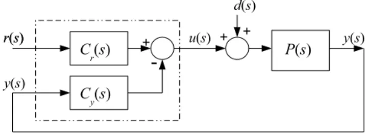
Consider the Two-Degree-of-Freedom (2-DoF) feedback control system of Fig. 1 whereP(s)is the controlled process transfer function, Cr(s) the set-point controller transfer
function,Cy(s)thefeedback controllertransfer function, and r(s) the set-point, d(s) the load-disturbance, and y(s) the controlled variable. The output of the 2-DoF controller is given by
u(s) =Cr(s)r(s)−Cy(s)y(s) (1)
For a P I2 controller [11] it is
u(s) =Kc
β+ 1
Tis
| {z }
Cr(s)
r(s)−Kc
1 + 1
Tis
| {z }
Cy(s)
y(s) (2)
whereKcis the controller gain,Tithe integral time constant,
andβ the set-point weighting factor (0≤β≤1).
The closed-loop control system response to a change in any of its inputs, will be given by
y(s) = Cr(s)P(s)
1 +Cy(s)P(s)
| {z }
Myr(s)
r(s) + P(s)
1 +Cy(s)P(s)
| {z }
Myd(s)
d(s) (3)
whereMyr(s)is the transfer function from set-point to
pro-cess variable: theservo-controlclosed-loop transfer function or complementary sensitivity functionT(s); and Myd(s) is
the one from load-disturbance to process variable: the reg-ulatory control closed-loop transfer function or disturbance sensitivity function Sd(s).
If β = 1, all parameters of Cr(s) are identical to the
ones of Cy(s). In such situation, it is impossible to specify
the dynamic performance of the control system to set-point changes, independently of the performance to load-disturbances changes. Otherwise, if the contrary, β < 1, given a controlled process P(s), the feedback controller
Cy(s) can be selected to achieve a target performance for
the regulatory control Myd(s), and then use the set-point
weighting factor in the set-point controllerCr(s), to modify
the servo-control performanceMyr(s).
The proposed Analytic Robust Tuning of Two-Degree-of-Freedom PI controllers (ART2) [12], [13], is aimed at producing a control system that responds fast and without oscillations to a step load-disturbance, with a maximum sensitivity lower than a specified value; in order to assure robustness; and which will also show a fast non-oscillating response to a set-point step change, not requiring strong or excessive control effort variations (smoothcontrol).
A. Outline of Controller Design Procedure
The first step in the Two-Degree-of-Freedom controller synthesis consists of obtaining the feedback controllerCy(s),
required to achieve a target Mt
yd(s) regulatory closed-loop
transfer function. From 3 once the controlled process is given and the target regulatory transfer function,Mt
yd(s), specified
the required feedback controller can be synthesized. The resulting feedback controller design equation is
Cy(s) =
P(s)−Mt
yd(s) P(s)Mt
yd(s)
= 1
Mt
yd(s)
−P1(s) (4)
Once, as a first step, the feedback controller Cy(s), is
obtained from 4, on a second step, the set-point controller
Cr(s)free parameter (β) can be used in order to modify the
servo control closed-loop transfer functionMyr(s).
III. TUNINGRULES FOR2-DOF PI CONTROL
Consider the First-Order-Plus-Dead-Time (FOPDT) con-trolled process given by
P(s) =Kpe−
Ls
T s+ 1 (5)
whereKpis the process gain,T the time-constant, andLits
dead-time. From here and after,τo=L/T will be referred
as the controlled processnormalized dead-time. In this work process models with normalized dead-time τo ≤ 2 are
considered. Processes with long dead-time will need some kind of dead-time compensation scheme (a Smith predictor, for example).
For the FOPDT process the specified regulatory control target closed-loop transfer function is chosen as
Mydt (s) =
Kse−Ls
(τcT s+ 1)2
(6)
and the closed-loop target function selected for the servo-control as
Mt
yr(s) =
e−Ls
τcT s+ 1
(7)
whereτc will be the dimensionless design parameter. It is
the ratio of the closed-loop control system time constant to the controlled process time constant.
A. Controller Parameters
In order to synthesize the 2-DoF PI controller for the FOPDT process it is necessary to use a rational function in s as an approximation of the controlled process dead-time. This approximation will affect the closed-loop response characteristics. Using the Maclaurin first order series for the dead-time
e−Ls
≈1−Ls (8)
and 5 and 6 in 4, the P I2 controller tuning equations are obtained as
κc=KcKp=
2τc−τc2+τo
(τc+τo)2
(9)
τi=
Ti
T =
2τc−τc2+τo
1 +τo
(10)
whereκc andτi are the controller normalized parameters.
In order to assure that the controller parameters 9 and 10 have positive values, the design parameter τc must be
selected within the range
0< τc ≤1 +
√
1 +τo (11)
The resulting regulatory control closed-loop transfer func-tion is
Myd(s) =
Tise−Ls Kc(τcT s+ 1)2
(12)
B. Set-point Weighting Factor
As the closed-loop transfer functions are related by
Myr(s) =Cyr(s)Myr(s), by using controllerCr(s),Myr(s)
can be written as
Myr(s) =
Kc(βTis+ 1)
Tis
Myd(s) (13)
Introducing in 13 the regulatory control closed-loop trans-fer function 12 and also the controller parameters 9 and 10, the servo-control transfer function then becomes
Myr(s) =
(βTis+ 1)e−Ls
(τcT s+ 1)2
(14)
As the servo-control target transfer function was specified in 7, from 7, 13 and 14 in order to obtain a non-oscillatory response, an adequate selection of the set-point weighting factor would beβ=τcT /Ti, and then
β= τcT
Ti
, 0< τc≤1 (15)
outside this range
β= 1, 1< τc<1 +
√
1 +τo (16)
This weighting factor also has influence in the controller output when the set-point changes. Effectively, the instan-taneous change on the control signal caused by a sudden change in the reference signal of magnitude∆ris given by
∆ur=Kcβ∆e=Kcβ∆r (17)
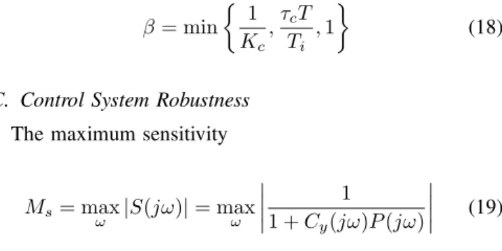
therefore, when very fast regulatory control responses are desired, high controller gain values are required, and the controller instantaneous output change when the set-point changes may be high. Then the controller output will be limited to be not greater than the total change on the set-point and then the set-set-point weighting factor selection criteria becomes
β= min
1
Kc
,τcT Ti
,1
(18)
C. Control System Robustness
The maximum sensitivity
Ms= max
ω |S(jω)|= maxω
1
1 +Cy(jω)P(jω)
(19)
will be used as an indication of the closed-loop control system robustness.
A robustness analysis has been performed. This analysis shows that the control system maximum sensitivity Ms
depends of the model normalized dead-timeτoand the design
parameterτc.
In order to avoid the loss of robustness when a very lowτc
is used, it is necessary to establish a lower limit to this design parameter. This relative loss of stability is greater when the normalized model dead-timeτo is high.
The design parameter lower limit for a given robustness level can be expressed in parameterized form as
τcmin=k1(Ms) +k2(Ms)τo (20)
where thek1 andk2 are show in Table I.
TABLE I EQUATION20 CONSTANTS
Ms 1.2 1.4 1.6 1.8 2.0
k1 0.4836 0.4152 0.3441 0.3254 0.3042 k2 1.8982 0.9198 0.6659 0.4853 0.3822
The design parameter equations (20) can be expressed as a single equation as
τcmin = k11(Ms) +
k21(Ms) k22(Ms)
τo (21)
k11(Ms) = 1.384−1.063Ms+ 0.262Ms2
k21(Ms) =−1.915 + 1.415Ms−0.077Ms2
k22(Ms) = 4.382−7.396Ms+ 3.0Ms2
Also it can be seen that; as usual; as the system becomes slower its robustness increases but if very slow responses are specified the system robustness starts to decrease, therefore the upper limit of the design parametersτc also needs to be
constrained By combining the design parameter performance and robustness constraints it may be selected within the range
max(0.50, τcmin)≤τc≤1.50 + 0.3τo (22)
IV. SIMPLIFIEDAUTOTUNINGRULES FOR2-DOF PI CONTROL
To provide the possibility of specify any possible desired robustness level within the range Ms ∈ [1.2 − 2.0] is
of great interest as this provides a complete view of the robustness-performance tradeoff and a quantified measure of how restrictive a robustness level can be depending on the process normalized dead-time. However, from a more practical point of view, the following question arises: When a desired Ms = 1.57 will be specified? With this respect,
as the Ms value is being recognized as ade factostandard
measure of robustness, an Ms value of 2.0 is recognized
as the minimum acceptable robustness level. This could be considered alowdegree of robustness. According to a similar measure, and in order to make the analysis simpler, amedium
degree of robustness is associated here withMs= 1.6while
a high degree of robustness will correspond to Ms = 1.4.
This broad classification allows a qualitative specification of the control system robustness.
According to this principle, the above mentioned three values of Ms are used here to generate the corresponding
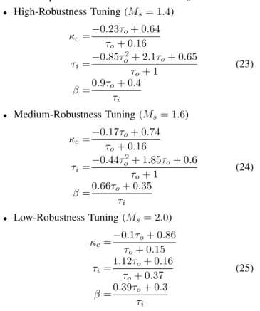
estimate for the lowest allowable closed-loop time-constant with 20 and introduce such time -constant value into the PI parameter equations (9), (10) and (15). The resulting controller parameters will be, in this case, expressed just in terms of the process normalized dead-timeτo as:
• High-Robustness Tuning (Ms= 1.4)
κc =−
0.23τo+ 0.64
τo+ 0.16
τi =−
0.85τ2
o+ 2.1τo+ 0.65
τo+ 1
(23)
β =0.9τo+ 0.4 τi
• Medium-Robustness Tuning (Ms= 1.6)
κc =−
0.17τo+ 0.74
τo+ 0.16
τi =−
0.44τ2
o+ 1.85τo+ 0.6
τo+ 1
(24)
β =0.66τo+ 0.35 τi
• Low-Robustness Tuning (Ms= 2.0)
κc=−
0.1τo+ 0.86
τo+ 0.15
τi=
1.12τo+ 0.16
τo+ 0.37
(25)
β=0.39τo+ 0.3 τi
Fig. 2 shows the generated values for a grid ofτo∈[0.1− 2.0] as well as the regression curves that gives rise to the above formulae for the normalized gain (κc) and integral
time (τi) as well as for the set-point weighting factor β.
V. EXAMPLES
Consider the FOPDT controlled process
P1(s) =
e−0.5s
s+ 1 (26)
0 0.5 1 1.5 2 0
0.5 1 1.5 2 2.5
Closed−Loop time constant τc
τo
0 0.5 1 1.5 2 0
0.5 1 1.5 2 2.5 3 3.5
Normalized gain κc
τo
0 0.5 1 1.5 2 0.4
0.5 0.6 0.7 0.8 0.9 1 1.1
Normalized integral time τi
τo 0 0.5 1 1.5 2
0 1 2 3 4 5
Set−point weighting β
τo o M
s = 1.4
+ M
s = 1.6
x Ms = 2.0
Fig. 2. PI Normalized Parameters for Low, Medium and High Robustness.
By using the full design equations, the controller param-eters and achieved robustness for different values of the desired closed-loop time constantτc are given in Table II.
TABLE II
EXAMPLE1 -ART2PI PARAMETERS
τc Kc Ti β Ms
0.6 1.11 0.98 0.67 1.75 0.8 0.86 0.97 0.82 1.49 1.2 0.51 0.97 1.0 1.26 1.4 0.37 0.89 1.0 1.20
As can be seen from Table II, to increase the control system robustness is necessary to decrease its speed. The designer may tackle the design problem in the inverse way, specifying the control system minimum robustness. Using the process normalize dead-time (τo= 0.5for this example)
and equations 20 and 22 the recommended lower limit for the design parameter to obtain a specified minimum robustness are estimated and listed in Table III.
TABLE III
DESIGNPARAMETERMINIMUMVALUES
Md
s 2.0 1.8 1.6 1.4 1.2
τcmin 0.5 0.567 0.677 0.875 1.433
In order to evaluate the performance of the simple tuning rules, the corresponding values ofMd
s are taken. The
con-troller parameters for the complete and autotuning relations are shown in Table IV.
TABLE IV
EXAMPLE1 - PI PARAMETERS; COMPLETE ANDAUTOTUNING
Complete Tuning Autotuning
Md
s Kc Ti β Kc Ti β
1.4 0.7914 0.9789 0.8688 0.7955 0.9917 0.8571 1.6 0.9958 0.7346 0.6864 0.9924 0.9333 0.7286 2.0 1.2547 0.8312 0.5978 1.2462 0.8276 0.5981
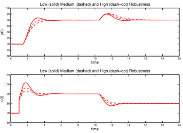
0 2 4 6 8 10 12 14 16 18 20 60
65 70 75 80 85 90 95 100
Low (solid) Medium (dashed) and High (dash−dot) Robustness
y(t)
time
0 2 4 6 8 10 12 14 16 18 20
60 70 80 90 100 110
Low (solid) Medium (dashed) and High (dash−dot) Robustness
u(t)
time
Fig. 3. Example 1 - System responses for the three robustness levels and comparing the complete and simple autotuning rules.
VI. CONCLUSIONS
An approach for automatic tuning of robust PI 2-DoF controller has been proposed. The method is analytically based; therefore called Analytical Robust Tuning (ART2); and starts from a First-Order-Plus-Dead-Time controlled process model to obtain a control system that responds fast and without oscillations to a step load-disturbance, with a maximum sensitivity lower than a specified value; in order to assure robustness; and which will also show a fast non-oscillating response to a set-point step change, not requiring strong or excessive control effort variations (smoothcontrol). Given a prescribed robustness level expressed in terms of the Maximum Sensitivity value (Ms), the lowest allowable
closed-loop time constant is determined. On that basis, the disturbance to output transfer function is matched and, on a second step, the control system performance to a set-point modified by an adequate selection of the Two-Degree-of-Freedom controller set-point weighting factorβ. The use of
β ≤1 values allows to decrease the servo-control response maximum overshot when very fast responses have been specified for the regulatory control. However, values larger than 1 may be generated if the system response is too slow. The resulting tuning can take any desired value for Ms as
the design parameter and generate, in a parameterized way, the three controller parameters (Kc,Ti andβ).
On the basis of the general approach, three different robustness levels are defined corresponding to the Maxi-mum Sensitivity values of: Ms = 1.4, Ms = 1.6 and Ms= 2.0. Simple tuning rules are generated by considering
these Ms values. The resulting autotuning rules provide
all the controller parameters parameterized in terms of the model normalized dead-time allowing the user to select for a High/Medium/Low Robust closed-loop system. The proposed autotuning expressions are therefore compared with other well known tuning rules also conceived with the same robustness spirit, showing the proposed approach is able to guarantee the same robustness level with an improvement of the system time performance.
Current research is conducted on the extension of the approach to a 2-DoF PID and to introduce alternative ways of designing the disturbance attenuation characteristics.
ACKNOWLEDGMENTS
This work has received financial support from the Spanish CICYT program under grant DPI2010-15230 and project AECI - PCI A/025100/09.
Also, the financial support from the University of Costa Rica and from the MICIT and CONICIT of the Government of the Republic of Costa Rica is greatly appreciated.
REFERENCES
[1] M. Ge, M. Chiu, and Q. Wang, “Robust PID Controller design via LMI approach,”Journal of Process Control, vol. 12, pp. 3–13, 2002. [2] R. Toscano, “A simple PI/PID controller design method via numerical optimization approach,”Journal of Process Control, vol. 15, pp. 81– 88, 2005.
[3] G. Silva, A. Datta, and S. Battacharayya, “New Results on the Synthesis of PID controllers,”IEEE Trans. Automat. Contr., vol. 47, no. 2, pp. 241–252, 2002.
[4] M. Ho and C. Lin, “PID controller design for Robust Performance,”
IEEE Trans. Automat. Contr., vol. 48, no. 8, pp. 1404–1409, 2003. [5] O. Arrieta and R. Vilanova, “PID Autotuning settings for balanced
Servo/Regulation operation,” in15th IEEE Mediterranean Conference on Control and Automation (MED07), June 27-29, Athens-Greece, 2007.
[6] S. Skogestad, “Simple analytic rules for model reduction and PID controller tuning,” Modeling, Identification and Control, vol. 25(2), pp. 85–120, 2004.
[7] M. Araki and H. Taguchi, “Two-Degree-of-Freedom PID Controllers,”
International Journal of Control, Automation, and Systems, vol. 1, pp. 401–411, 2003.
[8] T. H¨agglund and K. ˚Astr¨om, “Revisiting the Ziegler-Nichols tuning rules for PI control,”Asian Journal of Control, vol. 4(4), pp. 364– 380, 2002.
[9] K. ˚Astr¨om and T. H¨agglund, PID Controllers: Theory, Design and Tuning. Instrument Society of America, Research Triangle Park, NC, USA, 1995.
[10] D. Chen and D. E. Seborg, “PI/PID Controller Design Based on Direct Synthesis and Disturbance Rejection,”Ind. Eng. Cherm. Res., vol. 41, pp. 4807–4822, 2002.
[11] K. ˚Astr¨om and T. H¨agglund, Advanced PID Control. ISA - The Instrumentation, Systems, and Automation Society, 2006.
[12] V. M. Alfaro, “Analytical Tuning of Optimum and Robust PID Reg-ulators,” Master’s thesis, Escuela de Ingenier´ıa El´ectrica, Universidad de Costa Rica, 2006, (in Spanish).