Impact of Chaos Functions on Modern Swarm Optimizers.

Impact of Chaos Functions on Modern

Swarm Optimizers

E. Emary1,2, Hossam M. Zawbaa3,4*

1Department of Information Technology, Faculty of Computers and Information, Cairo University, Cairo, Egypt,2Computing Department, Faculty of Computer Studies, Arab Open University, Shrouq, Egypt, 3Department of Information Technology, Faculty of Computers and Information, Suef University, Beni-Suef, Egypt,4Department of Computer Science, Faculty of Mathematics and Computer Science, Babes-Bolyai University, Cluj-Napoca, Romania

*hossam.zawbaa@gmail.com

Abstract

Exploration and exploitation are two essential components for any optimization algorithm. Much exploration leads to oscillation and premature convergence while too much exploita-tion slows down the optimizaexploita-tion algorithm and the optimizer may be stuck in local minima. Therefore, balancing the rates of exploration and exploitation at the optimization lifetime is a challenge. This study evaluates the impact of using chaos-based control of exploration/ exploitation rates against using the systematic native control. Three modern algorithms were used in the study namely grey wolf optimizer (GWO), antlion optimizer (ALO) and moth-flame optimizer (MFO) in the domain of machine learning for feature selection. Results on a set of standard machine learning data using a set of assessment indicators prove advance in optimization algorithm performance when using variational repeated periods of declined exploration rates over using systematically decreased exploration rates.

1 Introduction

Chaos is the form of non-linear movement of the dynamics system and can experience any state according to its own regularity. Chaos has the ability of information processing that is applied widely in many fields like optimization problems, machine learning, and pattern recog-nition. The searching techniques based on chaos are similar to genetic algorithms (GA), but it uses the chaos variables. Because of the chaos is not repetition system, it can execute the overall search process in less computational time than stochastic ergodic techniques based on the probability [1]. Lately, the thought of applying the chaotic systems rather than random opera-tions has been observed in the optimization theory. The randomness role can be worked by chaotic motion rather than random processes in the optimization algorithms [2]. Numerous studies state as true that the advantages of applying the chaotic-based processes instead of ran-dom-based processes are usually visible despite the fact that a general principle can not be planned [3]. Chaos optimization algorithm (COA) has the chaos properties like ergodicity that can more efficiently escape from local minima than whatever other stochastic optimization algorithm [2]. COA utilizes the consistency exist as a part of a chaotic motion to escape from a11111

OPEN ACCESS

Citation:Emary E, Zawbaa HM (2016) Impact of Chaos Functions on Modern Swarm Optimizers. PLoS ONE 11(7): e0158738. doi:10.1371/journal. pone.0158738

Editor:Zhaohong Deng, Jiangnan University, CHINA

Received:March 31, 2016

Accepted:June 21, 2016

Published:July 13, 2016

Copyright:© 2016 Emary, Zawbaa. This is an open access article distributed under the terms of the

Creative Commons Attribution License, which permits unrestricted use, distribution, and reproduction in any medium, provided the original author and source are credited.

Data Availability Statement:Datasets are downloaded from the UCI Machine Learning Repository, [http://archive.ics.uci.edu/ml]. Irvine, CA: University of California, School of Information and Computer Science, 2013. All data sets names are available in Section 3, Results and Discussion (subsection 3.1 Data description).

local minima, but the random-based procedures escape from the local minima by perceiving some unacceptable solutions with a particular probability [2,4,5].

Over the previous years, the number of features in machine learning and pattern recogni-tion applicarecogni-tions have expanded from hundreds to thousands of input features. Feature selec-tion is a procedure for distinguishing the subset of significance features and remove the repetitive ones. Additionally, this technique is valuable when the size of input features is vast and not every one of them are required for describing the data [6]. Feature selection prompts the decrease of the dimensionality of features space that will enhance the classification perfor-mance. Moreover, it will help in better data understanding and reduce the computation time during the classification process [7,8]. There are two different techniques of feature selection approaches: filter-based and wrapper-based [9]. Thefilter-based approachsearches for a subset of features that optimize a given data-dependent criterion [10]. Thewrapper-based approach

applies the machine learning strategy as the evaluation component that has better results than the filter-based approach [11]; however, it is computationally costly [12].

Generally, feature selection is formulated as amulti-objectiveproblem with two goals: mini-mizethe number of selected features andmaximizethe classification performance. These two goals are conflicting and the optimal solution ought to adjust between them. A sort of search methods has been applied, for example, sequential forward selection (SFS) [13] and sequential backward selection (SBS) [14]. Nonetheless, these feature selection methods still experience the ill effects of stagnation in the local optima [15]. Evolutionary computing (EC) algorithms adap-tively search the space by using a set of search operators that contact in a social way to achieve the optimal solution [16,17].

The chaos genetic feature selection optimization method (CGFSO) investigates the search space with every conceivable combination of a given data set. Each individual in the population represents a candidate solution and the feature dimension is the same length as chromosomes length [18,19]. The chaotic time series with an EPNet algorithm requires a small network archi-tecture whereas the expansion of neural parts might debase the performance amid the evolution and gives more survival probabilities to smaller networks in the population [20,21]. The chaotic antlion optimization (CALO) can converge to the same optimal solution for a higher number of applications regardless of the stochastic searching and the chaotic adjustment [22].

In this paper, our aim is to propose an optimization algorithm based on two chaotic func-tions that employed to analyze their performance and impact on three bio-inspired optimiza-tion algorithms namely grey wolf optimizaoptimiza-tion (GWO), antlion optimizaoptimiza-tion (ALO), and moth-flame optimization (MFO). The rest of this paper is comprised as follows: Section 2 gives the foundation information of three used bio-inspired optimization algorithms and describes the usage of chaotic variants of GWO, ALO, and MFO in feature selection. Experimental results with discussions are displayed in Section 3 and the conclusions and future work are pro-vided in Section 4.

2 Materials and Methods

The following subsections provide the short brief of the applied three bio-inspired optimization algorithms and chaotic maps. After that, it describes the usage of chaotic variants of GWO, ALO, and MFO in feature selection.

2.1 Preliminaries

This subsection provides a brief summary of the three modern bio-inspired optimizers namely grey wolf optimization (GWO), antlion optimization (ALO), and moth-flame optimization (MFO). Moreover, we have provided a short introduction to the chaos theory.

1. Gray wolf optimization (GWO)

GWO is a relatively new optimization algorithm proposed by Mirjalili et al. in 2014 [23]. This algorithm mimics the hunting process of grey wolves. Grey wolves often live in a pack with strict leadership hierarchy.Table 1describes such hierarchy and the responsibility of each agent in the pack.

For a pack to hunt prey, a set of phases are to be applied in sequence [24]:

Prey encircling: the pack encircles a prey by repositioning individual agents according to the prey location. The encircling is modeled as in givenEq (1):

X

!

ðtþ1Þ ¼!XpðtÞ þA

!

:!D; ð1Þ

where!D is as defined inEq (2),tis the iteration number,!A and!C are coefficient vectors,

X

!

pis the prey position, and!X is the gray wolf position. D

!

¼ j!C:!X_pðtÞ !XðtÞj; ð2Þ

where!A,!C vectors are calculated as in Eqs(3)and(4).

A

!

¼2a:!r₁ a; ð3Þ

C

!

¼2r!2; ð4Þ

whereais linearly decreased from 2 to 0 over the course of iterations controllingexploration

andexploitation, andr1,r2are random vectors in [0, 1]. The value ofais the same for all

wolves in the pack.

By the end of encircling stage, the hunting stages start.

Hunting: is performed by the whole pack based on the information coming from the alpha, beta and delta wolves which are expected to know the prey location. Alpha, beta, and delta are assumed to have better knowledge about the potential location of prey and hence are used as guides for hunting. Individual wolf in the pack updates its position as shown in the

Eq (5):

X

!

ðtþ1Þ ¼ X1 !_{þ X}

2 !_{þ X}

3 !

3 ; ð5Þ

Table 1. The leadership hierarchy of the grey wolves pack.

Agent Responsibility

Alphas Decision making for the whole pack regarding hunting, sleeping,. . .etc. Beta Help the alpha in decision-making and candidate to be the alpha. Delta This group have many rules and classes such as:

•Scouts: Responsible for watching the boundaries of the territory and warning the pack in case of any danger.

•Sentinels protect and guarantee the safety of the pack.

•Elders are the experienced wolves who used to be alpha or beta.

•Hunters help the alphas and betas when hunting prey and providing food for the pack.

•Caretakers are responsible for caring for the weak, ill, and wounded wolves in the pack. Omega Babysitters in the pack and it is the last wolf allowed eating.

whereX!₁,X!₂,X!₃ are defined as in Eqs(6),(7)and(8)respectively.

X1 !_{¼ jX}

a

! _A

1 !_:D

a

!_{j; ð6Þ}

X2 !_{¼ jX}

b

! _A

2 !

:Db

!

j; ð7Þ

X3 !_{¼ jX}

d

! _A

3 !

:Dd !_j

; ð8Þ

whereX!_{a, X}

b

!_,X

d

!_{are thefirst three best solutions in the swarm at a given iterationt, A} 1 !_, A₂

!_,A 3 !_{are de}

fined as inEq (3), andD!_a,D!_b,D!_g are defined using Eqs(9),(10)and(11)

respectively.

Da !_{¼ jC}

1

!

:Xa ! !_Xj

; ð9Þ

Db !_{¼ jC}

2 !_:X

b

! !_{Xj; ð10Þ}

Dd !_{¼ jC}

3 !_:X

d

! !_{Xj; ð11Þ}

whereC!₁,C!₂, andC!₃ are defined as inEq (4).

By the end of preying stage, the pack attacks the prey in what is called attacking stage.

Attacking stage: the attacking phase is performed by allowing the agents to approach the prey which is achieved by decrementing the exploration rateaas outlined inEq 4witha2[1,2]. Byfinishing the attacking phase the pack is ready to search for a new prey which is the next phase.

Search for prey: in this phase, wolves diverge from each other tofind a new prey. This behav-ior is modeled by allowing large value for the parameterato allow for exploration of the search space as outlined inEq 4witha2[0, 1].

Algorithm 1 outlines the gray wolf optimization (GWO) algorithm.

Algorithm 1:Grey wolf optimization (GWO) algorithm

1:Inputs:nNumber of gray wolves in the pack,

NIterNumber of iterations for optimization.

2:Outputs:xαOptimal gray wolf position,

f(xα) Best fitness value.

3: Initialize a population ofngray wolves positions randomly. 4: Find theα,β, andδsolutions based on their fitness values. 5:whilestopping criteria is not metdo

6: for allWolfi2packdo

7: Update current wolf_’s position according toEq (5). 8: end for

9: Updatea,A, andCas in Eqs(2)and(3). 10: Evaluate the positions of individual wolves.

11: Updateα,β, andδpositions as in Eqs(9),(10)and(11). 12:end while

13: Select the optimal position (xα) and its fitness (f(xα)).

2. Antlion optimization (ALO)

agents utilized as a part of ALO algorithm to be specificantsandantlions. Antlion always dependably burrows a trap to chase ants, and when an ant falls in the hole, the antlion tosses sand towards it until it is slaughtered and ingested. After that, the antlion readies the trap again for the next chase.

In the artificial optimizer, the ants change their positions according to the antlions posi-tions. Individual ant performs two local searches around the elite antlion and the selected antlion; then updates itself position as the average of these two random walks as inEq (12):

Antt i ¼

Rt AþR

t E

2 ; ð12Þ

where_RtAis the random walk around the roulette wheel selected antlion, and_RtEis the ran-dom walk around the elite antlion.

The random walking of an ant_Xtant

iaround a given antlionXtantlionj

is modeled as in the

Eq (13):

Xt anti ¼

ðXi aiÞ ðdi c t iÞ

ðbt i aiÞ

þci; ð13Þ

where_Xtant

iis the updated ant numberiposition at iterationt,aiis the minimum of

ran-dom walk_Xtiini−thdimension, andbiis the maximum of random walkXtiini−th

dimension,Xiis defined inEq 14,canddare the lower and upper bounds of the random

walk.

XðtÞ ¼ ½0;cumsumð2rðt₁Þ 1Þ;cumsumð2rðt2Þ 1Þ;

:::;cumsumð2rðtTÞ 1ފ;

ð14Þ

wherecumsumcalculates the cumulative sum, andr(t) is a stochastic function characterized as in theEq (15):

rðtÞ ¼

1if rand>0:5

0if rand0:5;

(

ð15Þ

whererandis a random number created with uniform distribution in the interim of [0, 1].

canddparameters are adapted according to Eqs16and17to limit the range of the random walk around the given antlion.

ct i ¼

lb I þX

t

antlionj ifrand<0:5

lb I þX

t

antlionj otherwise;

8 > > > < > > > :

ð16Þ

dt i ¼

ub I þX

t

antlionj ifrand >0:5

ub I þX

t

antlionj otherwise;

8 > > > < > > > :

ð17Þ

rate and is defined inEq (18):

I¼10w t

T; ð18Þ

whereTis the maximum number of iterations,wis a constant characterized taking into account the present iteration (w= 2 whent>0.1T,w= 3 whent>0.5T,w= 4 when

t>0.75T,w= 5 whent>0.9T, andw= 6 whent>0.95T). The constantwcan modify the

accuracy level of exploitation.

Finally, the selection operation is applied where an antlion is replaced by an ant if the ant becomesfitter. As indicated by the above conditions ALO optimizer can be formulated as in the following algorithm 2.

Algorithm 2:Antlion optimization (ALO) algorithm

1:Inputs:nnumber of ants,

Nnumber of antlions,

Tmaximum number of iterations. 2:Outputs: The elitist antlion.

3: Initialize a population ofnant’s positions andNantlion’s positions randomly.

4: Calculate the fitness of all ants and antlions. 5: Find the fittest antlion (the elite).

6:t= 0.

7:whiletTdo

8: for allantido

9: Select an antlion utilizing the roulette wheel selection.

10: Slide ants towards the antlion; perform random pursuit around this selected antlion and normalize it.

11: Create a random walk forantiaround the elite antlion and normalize it.

12: Updateantiposition as the average of the two obtained random walks.

13: end for

14: Calculate the fitness of all ants.

15: Replace an antlion with its corresponding ant it if gets to be fitter. 16: Update elite if an antlion gets to be fitter than the elite.

17:end while

18: Select the elitist antlion and its fitness.

3. Moth-flame optimization (MFO)

Mirjalili proposed moth-flame optimization (MFO) in 2015 [26] that is motivated by the moths navigation approach. Moths depend ontransverse orientationfor navigation where a moth flies by keeping up a settled point concerning the moon. At the point when moths see the human-made artificial light, they endeavor to have a similar angle of the light to fly in the straight line. Moths and flames are the primary components of the artificial MFO algo-rithm. MFO is a population-based algorithm with the set ofnmoths are used as search operators. Flames are the bestNpositions of moths that are acquired so far. In this manner, every moth seeks around a flame and updates it if there should be an occurrence of finding a better solution. Given logarithmic spiral, a moth updates its position concerning a given flame as in theEq (19)[26]:

SðMi;FjÞ ¼Di:ebt:cosð2ptÞ þFj; ð19Þ whereDishows the Euclidian distance of thei−thmoth for thej−thflame,bis a constant

to define the shape of the logarithmic spiral,Midemonstrate thei−thmoth,Fjshows thej

As might be found in the above equation, the next position of a moth is characterized with respect to aflame. Thetparameter in the spiral equation describes how much the next posi-tion of the moth ought to be near theflame. The spiral equation permits a moth tofly around aflame and not necessarily in the space betweenflames taking into account both exploration and exploitation of solutions. With a specific end goal to further emphasize exploitation, we suppose thattis a random number in [r, 1] whereris linearly decreased from−1 to−2 through the span of emphasis and is called convergence constant. With this

technique, moths tend to exploit their correspondingflames more precisely corresponding to the number of iterations. In order to upgrade the likelihood of converging to a global solution, a given moth is obliged to update its position utilizing one of theflames (the corre-spondingflame). In every iteration and in the wake of updating theflame-list, theflames are sorted based on theirfitness values. After that, the moths update their positions as for their correspondingflames. To permit much exploitation of the best encouraging solutions, the number offlames to be taken after is diminished as for the iteration number as given in the

Eq (20):

Nflames¼round N l N 1

T

; ð20Þ

wherelis the present iteration number,Nis the maximum number offlames, andT demon-strates the maximum number of iterations. The moth-flame optimization (MFO) is exhib-ited in algorithm 3.

Algorithm 3:Moth-flame optimization (MFO) algorithm

1:Inputs:nnumber of moths,

Nnumber of flames,

Tmaximum number of iterations.

2:Outputs:Bestthe optimal flame position,

f(Best) the optimal flame fitness value.

3: Initialize a population ofnflames positions randomly in the search space.

4:whileStopping criteria is not metdo

5: Update theNnumber of flames as inEq (20). 6: Compute the fitness value for each moth. 7: iffirst iterationthen

8: Sort the moths from best to worst as per their fitness and place the result in the flame list.

9: else

10: Merge the population of past moths and flames. 11: Sort the merged population from best to worst.

12: Select the bestNpositions from the sorted merged population as the new flame list.

13: end if

14: Calculate the convergence constantr. 15: for allMothiwithindo

16: Computetast= (r−1)rand+ 1. 17: ifiNthen

18: UpdateMothiposition as indicated byFlameiapplyingEq (19).

19: else

20: UpdateMothiposition as indicated byFlameNusingEq (19).

21: end if

22: end for

23:end while

4. Chaotic maps

Chaotic systems are deterministic systems that display unpredictable (or even random) con-duct and reliance on the underlying conditions. Chaos is a standout amongst the most prominent phenomena that exist in nonlinear systems, whose activity is complex and like that of randomness [27]. Chaos theory concentrates on the conduct of systems that take after deterministic laws yet seem random and unpredictable, i.e., dynamical systems [16]. To be considered as chaotic, the dynamical system must fulfill the chaotic properties, for example, delicate to starting conditions, topologically blend, dense periodic orbits, ergodic, and stochastically intrinsic [28]. Chaotic components can experience all states in specific reaches as per their own particular consistency without redundancy [27]. Because of the ergodic and dynamic properties of chaos elements, chaos search is more fit for slope-climb-ing and gettslope-climb-ing away from local optima than the random search, and in this way, it has been applied for optimization [27]. It is generally perceived that chaos is a principal method of movement basic all common phenomena. A chaotic map is a guide that shows some sort of chaotic behavior [28]. The basic chaotic maps in the literature are:

a. Sinusoidal map:represented by theEq (21)[27]:

xkþ1¼a x 2

k sinðpxkÞ; ð21Þ which creates chaotic numbers in the range (0, 1) witha= 2.3.

b. Singer map:given in theEq (22)[29]:

xkþ1¼mð7:86xk 23:31x 2

kþ28:75x 3

k 13:3x 4

kÞ; ð22Þ withxk2(0,1) under the condition thatx02(0, 1),μ2[0.9, 1.08].

2.2 The proposed chaos-based exploration rate

As specified in [30], meta-heuristic optimization strategies dependably utilize high-level data to guide its trial and error mechanism for discovering satisfactory solutions. All meta-heuristic algorithms apply particular tradeoff of randomization and local search. Two noteworthy parts control the performance of a meta-heuristic algorithm to be specificexploitation (intensifica-tion) andexploration(diversification) [30]. Diversification intends to produce various solu-tions in order to investigate the search space on the large scale while intensification intends to concentrate on the pursuit in a local region by exploiting the data that an immediate decent solution is found in this area. The good combination of these two components will guarantee that the global optimality is achievable [30].

Some optimizers switches between exploration and exploitation gave some randomly gener-ated values, for example, bat algorithm (BA) [31] and flower pollination algorithm (FPA) [32]. Numerous late investigates done in the optimization area to use a single versatile equation to accomplish both diversification and intensification with various rates as in GWO [23], ALO [25], and MFO [26]. In the both cases, the optimizer begins with large exploration rate and iter-atively decrements this rate to improve the exploitation rate. The exploration rate takes after linear shape in GWO [23] and MFO [26] while it keeps the piece-wise linear shape in ALO [25]. In spite of the fact that exploration rate functions demonstrated proficient for tackling various optimization problems, despite this methodology has the following disadvantages:

enhancing the solutions that have as of now been found, regardless of the possibility that they are local optima.

2. Sub-optimal selection:toward the start of the optimization prepare, the optimizer has extremely exploration ability yet with this enhanced explorative force it might leave a prom-ising locale to less encouraging because of the oscillation and extensive training rates; see

Fig 1for such case in 1D representation.

These issues motivate using interleaved successive periods of exploration and exploitation all through the optimization time. In this way, when achieving a solution, the exploitation will be applied, followed by another exploration that permits the optimizer to jump to another promising region, then exploitation again to improve further the solution found. Chaotic sys-tems with their intriguing properties, for example, topologically blend, ergodicity, and intrinsic stochasticity, which can be applied to adjust the exploration rate parameter, taking into account the required equilibrium between the diversification and intensification [16].

The diversification rate in the native GWO is calledaand is linearly diminished from 2 to 0 throughout the course of iterations; as in theEq (4). Theaturns out to be under 1 to demon-strate the case that the wolf quit moving and approaches the prey. Along these lines, the follow-ing position of a wolf might be at any point between the wolf position and the prey position; seeFig 2[23]. At the point when the estimation ofais greater than 1, wolves separate from

Fig 1. An example of leaving the promising region for the less promising one in 1-D case.

doi:10.1371/journal.pone.0158738.g001

Fig 2. Exploration versus exploitation periods depending on the parameterain GWO [23].

each other to hunt down prey and merge to assault prey. Additionally, for the values greater than 1, the grey wolves are compelled to locate a fitter prey ideally; as inFig 2[23].

In ALO, the exploration or exploitation are controlled by contracting the span of updating ant’s positions and imitates the ant sliding procedure inside the pits by using the parameterIas appeared inFig 3. The span of ants’random walks hypersphere is decreased adaptively, and this behavior can be mathematically modeling as in theEq (23).

I¼10w t

T; ð23Þ

wheretis the present iteration,Tis the maximum number of iterations,wis a constant charac-terized taking into account the present iteration (w= 2 whent>0.1T,w= 3 whent>0.5T,

w= 4 whent>0.75T,w= 5 whent>0.9T, andw= 6 whent>0.95T). The constantwcan

conform the exactness level of exploitation.

In the case of MFO, theTparameter in the spiral equation characterizes how much the next position of the moth ought to be near (the corresponding) flame (T=−1 is the nearest position

to the flame whileT= 1 demonstrates the most remote one) as shown inFig 4. The spiral equa-tion permits a moth to fly around a flame and not as a matter of course in the space between them. In this manner, the exploration and exploitation of the search space can be ensured [26]. For switching between the exploration and exploitation operations, the parameterais charac-terized and linearly decremented amid the optimization from -1 to -2 to control the furthest reaches of theTvalue. The definite moth position in a given dimension is computed as given in

Eq (24).

T ¼ ða 1Þ randþ1; ð24Þ

whererandis a random number drawn from uniform distribution in the extent [0, 1] andais computed as in theEq (25).

a¼ 1þt frac 1MaxIter; ð25Þ wheretis the iteration number andMaxIteris the total number of iteration.

Fig 3. The shrinking of the random walk limits as per the parameterI[25].

In the proposed chaos adjustment of exploration rates, the adjustment of the parameterain GWO is controlled by the given chaos function; seeFig 5. A comparative strategy is utilized to adjust the parameterIthat confines the exploration rate in ALO; as in theFig 6. While the same conduct is applied to MFO where theaparameter controls the parametrictvalue that decides the moth position regarding the corresponding flame; as shown inFig 6. Two chaotic functions were used in this study to analyze their performance and impact on GWO, ALO, and MFO. The two chaotic functions have fit the progressive decrement of exploration and exploi-tation at successive periods are theSingerandSinusoidalfunctions which are embraced here as examples.

Fig 4. The possible positions of a given moth with respect to the corresponding flame [26].

doi:10.1371/journal.pone.0158738.g004

Fig 5. The Singer exploration rate versus the native exploration used as a part of GWO, ALO, and MFO.

2.3 Application of chaotic variants of GWO, ALO, and MFO for feature

selection

In this section, the proposed chaotic variations are employed in feature selection for classifica-tion problems. For a feature vector sizedN, the diverse feature subsets would be 2Nwhich is an immense space of features to be searchedexhaustively. Therefore, GWO, ALO, and MFO are used adaptively to explore the search space for best feature subset. The best feature subset is the one with greatestclassification performanceand leastnumber of selected features. The fitness function applied as a part of the optimizer to assess every grey wolf/antlion/moth position is as given by the followingEq (26):

Fitness¼a g_RðDÞ þb jC Rj

jCj ; ð26Þ

whereγ_R(D) is the classification performance of condition feature setRwith respect to choice

D,Ris the length of selected feature subset,Cis the aggregate number of features,αandβare two parameters relating to the significance of classification performance and subset length,α2

[0, 1] andβ= 1−α.

We can highlight that the fitness function maximizes the classification performance;γ_R(D), and the proportion of the unselected features to the aggregate number of features; as in the termjC R_jCjj. The above equation can be effectively changed over into a minimization by using the error rate as opposed to the classification performance and the selected features proportion as opposed to the unselected feature size. The minimization problem can be formulated as in the followingEq (27):

Fitness¼aERðDÞ þb

jRj

jCj; ð27Þ

whereER(D) is the error rate for the classifier of condition feature set,Ris the length of selected

feature subset, andCis the aggregate number of features.α2[0, 1] andβ= 1−αare constants

to control the significance of classification performance and feature selection;β= 0.01 in the current experiments.

The principle characteristic of wrapper-based in feature selection is the usage of the classi-fier as a guide during the feature selection procedure. K-nearest neighbor (KNN) is a super-vised learning technique that classifies the unknown examples and determined based on the minimum distance from the unknown samples to the training ones. In the proposed system, KNN is used as a classifier to guarantee the goodness of the selected features [33].

Fig 6. The Sinusoidal exploration rate versus the native exploration used as a part of GWO, ALO, and MFO.

3 Results and Discussion

3.1 Data description

21 datasets inTable 2from the UCI machine learning repository [34] are used as a part of the analyses and examinations results. The data sets were chosen to have different numbers of features and instances of the various problems that the proposed algorithms will be tried on.

In this study, the wrapper-based approach for feature selection is using the KNN classifier. KNN is used in the experiments based on trial and error basis where the best decision ofKis chosen (K= 5) as the best performing on all the data sets [33]. Through the training process, every wolf/antlion/moth position represents one solution (feature subset). The training set is used to assess the KNN on the validation set all through the optimization to guide the feature selection procedure. The test data are kept avoided the optimization and is let for final assess-ment. The global and optimizer-specific parameter setting is sketched out inTable 3. Every one of the parameters is set either as indicated by particular domain learning as theα,β

parameters of the fitness function or based on trial and error on small simulations or regular in the literature.

3.2 Evaluation criteria

Singular data sets are divided randomly into three different similar parts to be specific: training, validation, and testing sets in cross-validation manner. The apportioning of the data is repeated for 20 times to guarantee stability and statistical significance of the results. In every run, the fol-lowing measures are recorded from the validation data:

Table 2. Description of the data sets used in the study.

Data set No. features No. instances

Lymphography 18 148

WineEW 13 178

BreastEW 30 569

Breastcancer 9 699

Clean1 166 476

Clean2 166 6598

CongressEW 16 435

Exactly 13 1000

Exactly2 13 1000

HeartEW 13 270

IonosphereEW 34 351

KrvskpEW 36 3196

M-of-n 13 1000

PenglungEW 325 73

Semeion 265 1593

SonarEW 60 208

SpectEW 22 267

Tic-tac-toe 9 958

Vote 16 300

WaveformEW 40 5000

Zoo 16 101

• Classification performance: is a marker characterizes the classifier given the selected feature set and can be detailed as in theEq (28).

Performance¼ 1

M XM

j¼1 1 N

XN

i¼1

MatchðCi;LiÞ; ð28Þ

whereMis the number of times to run the optimization algorithm to choose the feature sub-set,Nis the number of samples in the test set,Ciis the classifier label for data samplei,Liis

the reference class label for data samplei, andMatchis a function that yields 1 when the two input labels are the same and produces 0 when they are distinctive.

• Mean fitness: is the average of solutions obtained from running an optimization algorithm for variousMrunning that can be given inEq (29).

Mean¼ 1

M XM

i¼1 gi

; ð29Þ

• Standard deviation (std) fitness: is a representation for the variety of the acquired best solu-tions found for running a stochastic optimizer forMdifferent times.Stdis employed as a pointer for the optimizer stability and robustness, thoughstdis smaller this implies that the optimizer always converges to the same solution; while bigger values forstdmean many ran-dom results as in theEq (30).

Std¼

ffiffiffiffiffiffiffiffiffiffiffiffiffiffiffiffiffiffiffiffiffiffiffiffiffiffiffiffiffiffiffiffiffiffiffiffiffiffiffiffiffiffiffiffiffiffiffi 1

M 1

X

ðgi

MeanÞ

2 r

; ð30Þ

whereMeanis the average characterized as in theEq (29).

• Selection features size: demonstrates the mean size of the selected features to the aggregate number of features as in theEq (31).

Selection¼ 1

M XM

i¼1 sizeðgi

Þ

D ; ð31Þ

wheresize(x) is the number of values for the vectorx, andDis the number of selected fea-tures in data set.

Table 3. Parameter setting for experiments.

Parameter Value(s)

No. of search agents 8

No. of iterations 100

Problem dimension No. of features in the data

Search domain [0 1]

No. Repetitions of runs 20

αparameter in thefitness function [0.9, 0.99]

βparameter in thefitness function 1—[0.9, 0.99]

inertia factor of PSO 0.1

• Wilcoxon rank-sum test: the null hypothesis is that the two examples originate from the same population, so any distinction in the two rank aggregates comes just from the inspecting error. The rank-sum test is described as the nonparametric version of thettest for two inde-pendent gatherings. It tests the null hypothesis that data inxandyvectors are samples from continuous distributions with equivalent medians against the option that they are not [35].

• T-test: is statistical importance demonstrates regardless of whether the contrast between two groups’midpoints in all probability mirrors a“real”distinction in the population from which the groups were inspected [36].

The three embraced optimizers were evaluated against their corresponding chaos controlled one where the three optimizers; GWO, ALO, and MFO were employed with two chaotic func-tions (SinusoidalandSinger) used as a part of the study. Also, the used optimizers and their chaotic variants are compared against one of the conventional optimizers namely particle swarm optimizer (PSO) [37].

3.3 Experimental results

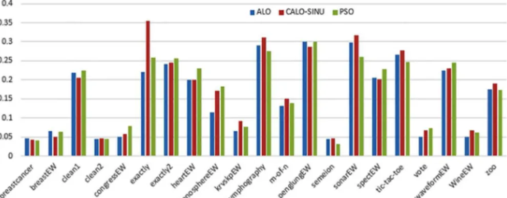
Figs7and8outline the performance of the native ALO versus its chaotic one where the singer and the sinusoidal function is employed in all 21 data sets. We can observe from the figures that the chaotic ALO version [22] is superior in performance to the native ALO performance on most of the data set regardless of the used chaotic function. Comparable results are

Fig 7. Mean fitness values for the ALO versus CALO using the Singer function.

doi:10.1371/journal.pone.0158738.g007

Fig 8. Mean fitness values for the ALO versus CALO using the Sinusoidal function.

illustrated in Figs9and10applying the GWO. In the case of MFO, less enhance in perfor-mance is remarked where the chaotic and the native MFO have practically identical results as shown in Figs11and12. The principle purpose behind this, a random value is utilized to choose the position of a moth that is joined with the used exploration rate, so it decreases its

Fig 9. Mean fitness values for the GWO versus CGWO using the Singer function.

doi:10.1371/journal.pone.0158738.g009

Fig 10. Mean fitness values for the GWO versus CGWO using the Sinusoidal function.

doi:10.1371/journal.pone.0158738.g010

Fig 11. Mean fitness values for the MFO versus CMFO using the Singer function.

effect. Besides, the native MFO is relied upon to give variability in exploration toward the end stages of the optimization as found inFig 13.Fig 13demonstrates the conceivable positions for a moth in given dimension where the flame is situated at 1 while the moth is initially situated at 0 in that dimension at the differentavalues. We can highlight from the figure that it conceiv-able to provide exploration and exploitation at all the optimization stages and henceforth there is no improve in performance for the chaotic MFO.

Comparative conclusions and comments can be found in Figs14–19that outline the perfor-mance of the selected features by the different optimizers on the test data. Moreover, we can remark that there is clear progress in performance for using chaotic versions with both ALO and GWO while the native MFO has practically identical performance on test data with it cha-otic version. For assessing optimizer repeatability and capability to convergence to the global optimal regardless of the initial positioning of search agents, we have employed the standard deviation (std) of the acquired fitness function value over all the runs for the different optimiz-ers. Figs20–22outline the obtained std values for the native and chaotic variants of three used optimizers. We can highlight from the figures that the chaotic versions of the optimizers have practically comparable std values in spite of the fact that they rely on upon chaotic functions as opposed to systematic functions which motivate using such models.

Fig 12. Mean fitness values for the MFO versus CMFO using the Sinusoidal function.

doi:10.1371/journal.pone.0158738.g012

Fig 13. Possible positions for a moth using the different values for the a parameter.

The secondary objective in the used fitness function is minimizing the number of selected features. Tables4–6. We can remark that the three optimizers with their variants can optimize the number of selected features as well as improve the classifier performance. We can notice that this secondary objective is much achieved in the case of using the chaotic variants as the

Fig 14. Average classification performance for the ALO versus CALO using the Singer function.

doi:10.1371/journal.pone.0158738.g014

Fig 15. Average classification performance for the ALO versus CALO using the Sinusoidal function.

doi:10.1371/journal.pone.0158738.g015

Fig 16. Average classification performance for the GWO versus CGWO using the Singer function.

chaos allows the algorithms to continue exploring the space for the better solution even in the final periods of the optimization process. For assessing the significance of performance of the optimizers and their corresponding chaotic variants both thet-testand theWilixicontest were measured inTable 7.Table 7demonstrates the significant advance in utilizing the chaotic ver-sion of the ALO and GWO at a significance level of 0.05 while there is no remarkable progress

Fig 18. Average classification performance for the MFO versus CMFO using the Singer function.

doi:10.1371/journal.pone.0158738.g018

Fig 17. Average classification performance for the GWO versus CGWO using the Sinusoidal function.

doi:10.1371/journal.pone.0158738.g017

Fig 19. Average classification performance for the MFO versus CMFO using the Sinusoidal function.

in using the chaotic variant of MFO. A comparable conclusion can be derived from remarking the p-value of the t-test where the chaotic variant of ALO and GWO are much clear while there is no reasonable improve in performance for using the chaotic variant of MFO.

When using different weights of objectivesαandβin the fitness function, we change the priority of each objective in the optimization process. Changing such weights affect the shape of the objective function and hence affects the performance of the used optimizers. The change in the shape of fitness function can result in appearance/disappearance of local minima and/or change of the global optima for such fitness function. Figs23–25depict the impact of changing the weight factorαon the performance of individual optimizers. We set the range of change of theαparameter to the range [0.99, 0.9] and theβparameter is set as 1−αas the rational Fig 20. Standard deviation (std) of the obtained optimal fitness values for ALO versus CALO using the Singer and Sinusoidal functions.

doi:10.1371/journal.pone.0158738.g020

Fig 21. Standard deviation (std) of the obtained optimal fitness values for GWO versus CGWO using the Singer and Sinusoidal functions.

setting. The figures display the obtained sum of fitness function values obtained by the 10 dif-ferent employed optimizers over all the data sets used. We can view from the figures that the chaotic versions of the optimizers still performs well with changing the shape of the fitness function which prove the capability of such variant to tolerate local optimal and convergence to a global one.

Fig 22. Standard deviation (std) of the obtained optimal fitness values for MFO versus CMFO using the Singer and Sinusoidal functions.

doi:10.1371/journal.pone.0158738.g022

Table 4. Average selection features size for the chaotic and native ALO over all the data sets.

Data CALO-SING ALO PSO CALO-SIN

Breastcancer 0.444 0.519 0.519 0.481

BreastEW 0.500 0.478 0.456 0.522

Clean1 0.329 0.456 0.462 0.442

Clean2 0.510 0.679 0.518 0.661

CongressEW 0.104 0.167 0.375 0.200

Exactly 0.564 0.641 0.615 0.569

Exactly2 0.538 0.077 0.385 0.282

HeartEW 0.718 0.590 0.538 0.667

IonosphereEW 0.069 0.088 0.402 0.401

KrvskpEW 0.550 0.583 0.426 0.569

Lymphography 0.333 0.315 0.407 0.204

M-of-n 0.615 0.795 0.590 0.674

PenglungEW 0.089 0.190 0.425 0.317

Semeion 0.377 0.519 0.472 0.447

SonarEW 0.506 0.528 0.439 0.456

SpectEW 0.121 0.318 0.333 0.242

Tic-tac-toe 0.667 0.889 0.556 0.826

Vote 0.104 0.208 0.458 0.317

WaveformEW 0.733 0.883 0.575 0.767

WineEW 0.667 0.667 0.590 0.592

Zoo 0.375 0.479 0.354 0.417

Table 5. Average selection features size for the chaotic and native GWO over all the data sets.

Data CGWO-SING ALO PSO CGWO-SIN

Breastcancer 0.444 0.519 0.519 0.519

BreastEW 0.367 0.478 0.456 0.267

Clean1 0.263 0.456 0.462 0.315

Clean2 0.259 0.679 0.518 0.373

CongressEW 0.354 0.167 0.375 0.125

Exactly 0.410 0.641 0.615 0.410

Exactly2 0.205 0.077 0.385 0.154

HeartEW 0.359 0.590 0.538 0.385

IonosphereEW 0.255 0.088 0.402 0.304

KrvskpEW 0.250 0.583 0.426 0.370

Lymphography 0.241 0.315 0.407 0.204

M-of-n 0.487 0.795 0.590 0.487

PenglungEW 0.191 0.190 0.425 0.160

Semeion 0.338 0.519 0.472 0.341

SonarEW 0.256 0.528 0.439 0.261

SpectEW 0.182 0.318 0.333 0.212

Tic-tac-toe 0.593 0.889 0.556 0.556

Vote 0.208 0.208 0.458 0.188

WaveformEW 0.392 0.883 0.575 0.375

WineEW 0.410 0.667 0.590 0.410

Zoo 0.271 0.479 0.354 0.313

doi:10.1371/journal.pone.0158738.t005

Table 6. Average selection features size for the chaotic and native MFO over all the data sets.

Data CMFO-SING ALO PSO CMFO-SIN

Breastcancer 0.407 0.519 0.519 0.481

BreastEW 0.489 0.478 0.456 0.467

Clean1 0.500 0.456 0.462 0.490

Clean2 0.528 0.679 0.518 0.514

CongressEW 0.542 0.167 0.375 0.479

Exactly 0.718 0.641 0.615 0.513

Exactly2 0.513 0.077 0.385 0.385

HeartEW 0.615 0.590 0.538 0.513

IonosphereEW 0.412 0.088 0.402 0.471

KrvskpEW 0.435 0.583 0.426 0.472

Lymphography 0.389 0.315 0.407 0.407

M-of-n 0.487 0.795 0.590 0.462

PenglungEW 0.456 0.190 0.425 0.416

Semeion 0.501 0.519 0.472 0.494

SonarEW 0.517 0.528 0.439 0.422

SpectEW 0.485 0.318 0.333 0.318

Tic-tac-toe 0.556 0.889 0.556 0.556

Vote 0.604 0.208 0.458 0.292

WaveformEW 0.525 0.883 0.575 0.575

WineEW 0.564 0.667 0.590 0.436

Zoo 0.458 0.479 0.354 0.479

4 Conclusions

In this study, two chaos functions were employed to control the exploration rate for three of the modern bio-inspired optimization algorithms. The fundamental assumption of the work evaluates the impact of using such chaos functions as a replacement for the originally used lin-ear or quasi-linlin-ear functions. The study evaluates the proposed two chaotic versions of the algorithms as well as the original ones in the domain of machine learning for feature selection. The results were conducted on a set of data sets drawn from the UCI repository and were assessed using different assessment indicators. The study found that utilizing exploration with high rate toward the end stages of optimization offers the algorithm some assistance with

Table 7. Significance tests for optimizers pairs.

Optimzer_1 Optimizer_2 Wilcoxon T-test

MFO MFO-Sin. 0.699 0.202

MFO MFO-Singer 0.589 0.030

MFO PSO 0.058 0.049

MFO-Sin. PSO 0.05 0.048

MFO-Singer PSO 0.047 0.049

GWO GWO-Sin. 0.072 0.034

GWO GWO-Singer 0.050 0.027

GWO PSO 0.049 0.046

GWO-Sin. PSO 0.043 0.048

GWO-Singer PSO 0.037 0.039

ALO ALO-Sin. 0.081 0.046

ALO ALO-Singer 0.026 0.038

ALO PSO 0.044 0.045

ALO-Sin. PSO 0.048 0.044

ALO-Singer PSO 0.047 0.049

doi:10.1371/journal.pone.0158738.t007

Fig 23. Fitness sum over all the used data sets for CALO versus ALO and PSO at a different setting of

α.

avoiding the local optima and premature convergence. Additionally, using the exploitation with high rate at the beginning of optimization helps the algorithm to select the most promis-ing regions in the search space. Henceforth, the paper proposes uspromis-ing successive periods of exploration and exploitation during the optimization time. The chaos functions are the illustra-tion of such funcillustra-tions that can provide successive exploraillustra-tion and exploitaillustra-tion and thus it pro-vides excellent performance when used with GWO and ALO.

Acknowledgments

This work was partially supported by the IPROCOM Marie Curie initial training network, funded through the People Programme (Marie Curie Actions) of the European Union’s Sev-enth Framework Programme FP7/2007-2013/ under REA grant agreement No. 316555.

Fig 24. Fitness sum over all the used data sets for CGWO versus GWO and PSO at a different setting ofα.

doi:10.1371/journal.pone.0158738.g024

Fig 25. Fitness sum over all the used data sets for CMFO versus MFO and PSO at a different setting of

α.

Author Contributions

Conceived and designed the experiments: EE HMZ. Performed the experiments: EE. Analyzed the data: HMZ. Contributed reagents/materials/analysis tools: HMZ EE. Wrote the paper: HMZ EE.

References

1. Wang D.F., Han P., Ren Q.,“Chaos Optimization Variable Arguments PID Controller And Its Applica-tion To Main System Pressure Regulating System”, First International Conference On Machine Learn-ing And Cybernetics, BeijLearn-ing, November, 2002.

2. Tavazoei M.S., Haeri M.“An optimization algorithm based on chaotic behavior and fractal nature”, Computational and Applied Mathematics, Vol. 206, pp. 1070–1081, 2007. doi:10.1016/j.cam.2006.09. 008

3. Bucolo M., Caponetto R., Fortuna L., Frasca M., Rizzo A.,“Does chaos work better than noise”, Circuits and Systems Magazine, IEEE, Vol. 2, No. 3, pp. 4–19, 2002. doi:10.1109/MCAS.2002.1167624

4. Li B., Jiang W.,“Optimization complex functions by chaos search”, Cybernetics and Systems, Vol. 29, No. 4, pp. 409–419, 1998. doi:10.1080/019697298125678

5. Yang J.J., Zhou J.Z., Wu W., Liu F., Zhu C.J., Cao G.J.,“A chaos algorithm based on progressive opti-mality and Tabu search algorithm”, International Conference on Machine Learning and Cybernetics, Vol. 5, pp. 2977–2981, 2005.

6. Chizi B., Rokach L., Maimon O.,“A Survey of Feature Selection Techniques”, IGI Global, pp. 1888–

1895, 2009.

7. Chandrashekar G., Sahin F.,“A survey on feature selection methods”, Computers & Electrical Engi-neering, Vol. 40, No. 1, pp. 16–28, 2014. doi:10.1016/j.compeleceng.2013.11.024

8. Huang C.L.,“ACO-based hybrid classification system with feature subset selection and model parame-ters optimization”, Neurocomputing, Vol. 73, pp. 438–448, 2009. doi:10.1016/j.neucom.2009.07.014

9. Kohavi R., John G.H.,“Wrappers for feature subset selection”, Artificial Intelligent, Vol. 97, No. 1, pp. 273–324, 1997. doi:10.1016/S0004-3702(97)00043-X

10. Chuang L.Y., Tsai S.W., Yang C.H.,“Improved binary particle swarm optimization using catsh effect for attribute selection”, Expert Systems with Applications, Vol. 38, pp. 12699–12707, 2011.

11. Xue B., Zhang M., Browne W.N.,“Particle swarm optimisation for feature selection in classification: Novel initialisation and updating mechanisms”, Applied Soft Computing, Vol. 18, PP. 261–276, 2014. doi:10.1016/j.asoc.2013.09.018

12. Guyon I., Elisseeff A.,“An introduction to variable and attribute selection”, Journal of Machine Learning Research, Vol. 3, pp. 1157–1182, 2003.

13. Whitney A.,“A direct method of nonparametric measurement selection”, IEEE Trans. Comput. Vol. C-20, No. 9, pp. 1100–1103, 1971. doi:10.1109/T-C.1971.223410

14. Marill T., Green D.,“On the effectiveness of receptors in recognition systems”, IEEE Trans. Inf. Theory, Vol. IT-9, No. 1, pp. 11–17, 1963. doi:10.1109/TIT.1963.1057810

15. Bing X., Zhang M., Browne W.N.,“Particle swarm optimization for feature selection in classification: a multi-objective approach”, IEEE transactions on cybernetics, Vol. 43, No. 6, pp. 1656–1671, 2013. doi:

10.1109/TSMCB.2012.2227469

16. Hassanien A.E., Emary E.,“Swarm Intelligence: Principles, Advances, and Applications”, CRC Press, Taylor & Francis Group, 2015.

17. Shoghian S., Kouzehgar M.,“A Comparison among Wolf Pack Search and Four other Optimization Algorithms”, World Academy of Science, Engineering and Technology, Vol. 6, 2012.

18. Oh I.S., Lee J.S., Moon B.R.,“Hybrid genetic algorithms for feature selection”, IEEE Transactions on Pattern Analysis and Machine Intelligence, Vol. 26, No. 11, pp. 1424–1437, 2004. doi:10.1109/ TPAMI.2004.105

19. Chen H., Jiang W., Li C., Li R.,“A Heuristic Feature Selection Approach for Text Categorization by Using Chaos Optimization and Genetic Algorithm”, Mathematical Problems in Engineering, Vol. 2013, 2013.

20. Gholipour A., Araabi B.N., Lucas C.,“Predicting chaotic time series using neural and neurofuzzy mod-els: A comparative study”, Neural Processing Letters, Vol. 24, No. 3, pp. 217–239, 2006. doi:10.1007/ s11063-006-9021-x

22. Zawbaa H.M., Emary E., Grosan C.,“Feature selection via chaotic antlion optimization”, PLoS ONE, Vol. 11, No. 3, e0150652, 2016. doi:10.1371/journal.pone.0150652

23. Mirjalili S., Mirjalili S.M., Lewis A.,“Grey Wolf Optimizer”, Advances in Engineering Software, Vol. 69, pp. 46–61, 2014. doi:10.1016/j.advengsoft.2013.12.007

24. Emary E., Zawbaa H.M., Grosan C., Hassanien A.E.,“Feature subset selection approach by Gray-wolf optimization”, 1st International Afro-European Conference For Industrial Advancement, Ethiopia, November, 2014.

25. Mirjalili S.,“The Ant Lion Optimizer”, Advances in Engineering Software, Vol. 83, pp. 83–98, 2015. doi:

10.1016/j.advengsoft.2015.01.010

26. Mirjalili S.,“Moth-Flame Optimization Algorithm: A Novel Nature-inspired Heuristic Paradigm”, Knowl-edge-Based Systems, Vol. 89, pp. 228–249, 2015. doi:10.1016/j.knosys.2015.07.006

27. Ren B., Zhong W.,“Multi-objective optimization using chaos based PSO”, Information Technology, Vol. 10, No. 10, pp. 1908–1916, 2011. doi:10.3923/itj.2011.1908.1916

28. Vohra R., Patel B.,“An Efficient Chaos-Based Optimization Algorithm Approach for Cryptography”, Communication Network Security, Vol. 1, No. 4, pp. 75–79, 2012.

29. Aguirregabiria J.M.,“Robust chaos with variable Lyapunov exponent in smooth one-dimensional maps”, Chaos Solitons & Fractals, Vol. 42, No. 4, pp. 2531–2539, 2014. doi:10.1016/j.chaos.2009.03. 196

30. Yang X.S.,“Nature-Inspired Metaheuristic Algorithms”, Luniver Press, 2nd edition, 2010

31. Yang X.S.,“A New Metaheuristic Bat-Inspired Algorithm”, Nature Inspired Cooperative Strategies for Optimization (NISCO), Studies in Computational Intelligence, Springer, Vol. 284, pp. 65–74, 2010. 32. Yang X.S.,“Flower pollination algorithm for global optimization”, Unconventional Computation and

Nat-ural Computation, Lecture Notes in Computer Science, Vol. 7445, pp. 240–249, 2012. doi:10.1007/ 978-3-642-32894-7_27

33. Yang C.S., Chuang L.Y., Li J.C., Yang C.H.,“Chaotic Binary Particle Swarm Optimization for Feature Selection using Logistic Map”, IEEE Conference on Soft Computing in Industrial Applications, pp. 107–

112, 2008.

34. Frank A., Asuncion A.,“UCI Machine Learning Repository”, 2010.

35. Wilcoxon F.,“Individual Comparisons by Ranking Methods”, Biometrics Bulletin, Vol. 1, No. 6. pp. 80–

83, 1945. doi:10.2307/3001968

36. Rice J.A.,“Mathematical Statistics and Data Analysis”, 3rd edition, Duxbury Advanced, 2006. 37. Kennedy J., Eberhart R.,“Particle swarm optimization”, IEEE International Conference on Neural