J. Braz. Soc. Mech. Sci. & Eng. vol.28 número4

Peter C. Müller

mueller@srm.uni-wuppertal.de Safety Control Engineering University of Wuppertal D-42097 Wupperta. Germany

Modified Lyapunov Equations for LTI

Descriptor Systems

For linear time-invariant (LTI) state space systems it is well-known that its asymptotic stability can be related to solution properties of the Lyapunov matrix equation according to so-called inertia theorems. The question now arises how analogous results can be obtained for LTI descriptor systems (singular systems, differential-algebraic equations). The stability behaviour of a LTI descriptor system is characterized by the eigenvalues of the related matrix pencil. Additionally, by a quadratic Lyapunov function the stability problem can be discussed by solution properties of a generalized Lyapunov matrix equation including a singular coefficient matrix. To overcome this difficult problem of singularity, the Lyapunov matrix equation will be modified such that a regular Lyapunov matrix equation appears and asymptotic stability is preserved. This aim can be reached by shifting the system matrices in a well defined manner. For that the a priori knowledge of an upper bound of the eigenvalues is assumed. It will be discussed how to get such bound. The paper ends with an inertia theorem where the solution properties of a regular modified Lyapunov matrix equation are uniquely related to the asymptotic stability of the LTI descriptor system.

Keywords: Descriptor systems, asymptotic stability, Lyapunov matrix equations, inertia theorem

Introduction

For linear time-invariant state space systems xɺ(t)=Ax(t) it is well known that its asymptotic stability can be discussed by inertia theorems for the Lyapunov matrix equation ATP+AP=−Q, cf. (Müller, 1977). The question now arises how analogous results can be obtained for descriptor systems. In the last two decades the modelling of dynamical systems by descriptor systems (singular systems, differential-algebraic equations) became more and more familiar leading to.1

x dim n 1 rkE ), t ( Ax ) t ( x

Eɺ = = < = (1)

for linear time-invariant systems where x is an n-dimensional generalized state vector (descriptor vector) and E is a quadratic singular matrix. It is assumed that the related matrix pencil

) A E

(λ − is regular, i.e. det(λE−A)≠0. Then system (1) can be decomposed in a “slow” and in a “fast” subsystem: there exist two regular matrices R S such that ,



    

=

     

=

2 1 1

I A RAS , N I

RES (2)

where N is a nilpotent matrix of degree k which is called the index of the descriptor system (1). Then the

decomposition is represented by

     

=

2 1 x x S x

) t ( x ) t ( x N ), t ( x A ) t (

xɺ1 = 1 1 ɺ2 = 2

, n n n , n ) x

dim( i = i 1+ 2= (3)

Presented at XI DINAME – International Symposium on Dynamic Problems of Mechanics, February 28th - March 4th, 2005, Ouro Preto. MG. Brazil. Paper accepted: June, 2005. Technical Editors: J.R.F. Arruda and D.A. Rade.

where the x - and the ₁ x - subsystems are called the slow and the 2 fast subsystem, correspondingly, cf. (Dai, 1989).

Mechanical Descriptor Systems

Lagrange’s equations of the first and second kinds are well established in analytical mechanics. They describe the dynamic behaviour of discrete systems, particularly of multibody systems. The difference between the two kinds consists in the manipulation of the kinematic constraints. If a kinematic description of the system has been given in generalized coordinates which are consistent with the constraints, the Lagrange’s equations of the second kind can be derived, leading to a set of differential equations only. However, if a redundant set of coordinates is used to describe kinematically the system containing still some constraints explicitly, then Lagrange’s equations of the first kind follow. For LTI multibody systems these equations result in

2 T 1 T

G F ) t ( Kq ) t ( q D ) t ( q

Mɺɺ + ɺ + = λ + λ (4)

, 0 ) t (

Fq = holonomic constraints, (5)

, 0 ) t ( Hq ) t ( q

Gɺ + = nonholonomic constraints. (6)

Here, q represents the q-dimensional displacement vector, M, D, K stand for the mass matrix, the dissipative and gyroscopic matrix, and the displacement and circulatory matrix, correspondingly. The f- and g-dimensional vectors λ1 and λ2 characterize the Lagrange’s multipliers (constraint forces) due to the constraints (5) and (6).

The first order representation of section 1.1 is obtained by defining the descriptor vector

T 2 T 1 T T T

q q

x = ɺ λ λ (7)

q

I

M E

0 0

= ,

0 0 G H

0 0 0 F

G F D K

0 0 I 0

A

T T q

− −

= (8)

The equations (4-6) are represented equivalently by Eq. (1) using the expressions (7,8).

It should be mentioned that some properties of the system (4-6) can be characterized by certain system conditions. (1) The matrix pencil

((((

λE−−−−A

))))

is assumed to be regular:det(λE−−−−A)≠≠≠≠0. For that it is necessary that

g f

rank = +

G F

(9)

holds.

(2) The classification of independent holonomic and nonholonomic constraints requires the necessary and sufficient

Conditions

rank = f +g G F

, rank = f+g H F

(10)

(3) The existence of a unique static equilibrium 0

, 0 , 0

q==== λ₁==== λ₂==== is guaranteed by

g f q

rank = + +

− −

0 0 H

0 0 F

G F

K T T

(11)

or equivalently by Eq. (10) and

(

f g

)

q

rank _= − +

  

  

−

    

  

−

+ +

H F H

F I K G

F G F

I _q

T T

q (12)

where (.)+ means the Moore-Penrose inverse of a matrix (.).

The remarks (1), (2), (3) represent a series of requirements in ascending order. If Eq. (11) is satisfied, then the equations (10) and (9) are satisfied also.

Mechanical descriptor systems (4-6) are a special but important application of the general descriptor systems (1) of

which the asymptotic stability will be considered in detail.

Asymptotic Stability

The stability behaviour of Eq. (1) is defined by the eigenvalues of the matrix pencil

((((

λE−−−−A

))))

which coincide with the eigenvalues of the system matrix A of the slow subsystem. By the quadratic ₁

Lyapunov function υ====₂1xTPExthe stability problem can be also

discussed by solution properties of the generalized Lyapunov matrix equation

Q PA E PE

AT ++++ T ====−−−− . (13)

Now the problem arises how the asymptotic stability of (1), i.e.

((((

0

))))

Reλi<<<< for all eigenvalues of A , relates to solution properties 1

of Eq. (13), i.e. how inertia theorems can be developed for linear time-invariant descriptor systems.

Because the matrix E is singular, the matrix Q can not be chosen as a regular matrix. The singularity of E results in a difficult problem for the solution of Eq. (13). Until now, only special inertia theorems are known. The results of Ishihara and Terra (2002) are restricted to systems of index k = 1 (which excludes mechanical descriptor systems with holonomic constraints being of index k = 3), where (Ishihara and Terra, 2002) gives some corrections of (Lewis, 1986). The results of Müller (1993), Owens and Debeljkovic (1985), Stykel (2002 a, 2002 b) require the calculation of the transformation matrices R , S of Eq. (2). But then A1 of the slow subsystem is also known and the stability behaviour can be discussed by A directly. ₁

Recently in (Wang et al, 2002) a new aspect for the stability discussion of system (1) has been introduced. If the fast subsystem, cf. Eq. (3), is replaced by an asymptotically stable subsystem with finite eigenvalues, then the stability properties of system (1) remain unchanged. This replacement can be achieved by changing E into a suitable regular matrix E⌢. Unfortunately, this procedure for determining E⌢ again requires the matrices R, S which is disadvantageous as mentioned above. But nevertheless, we shall follow this idea.

Modified System

The aim is to modify the system (1) into a system with the

matrix pencil

((((

λEˆ−−−−Aˆ

))))

such that

- Eˆ is regular leading to a "regular" Lyapunov matrix equation (19),

- asymptotic stability is preserved,

- the transformation matrices R , S are not required. Assuming a linear modification

E A Aˆ , A E

Eˆ ==== −−−−α ==== ++++β (14)

the infinite eigenvalues of system (1) correspond to

λˆi∞∞∞∞====−−−−_α1 <<<<0 forα>>>>0, i====1,...,n2 (15)

of the modified system. The finite eigenvalues of system (1), i.e. the

eigenvalues of A , relate to eigenvalues ₁ λˆ_jof the matrix pencil

(

λEˆ−Aˆ

)

by

1 j

1 ˆ ˆ

j , ˆ 1 0, j 1,...,n

j j

==== ≠≠≠≠ ++++ ====

−−−− −−−−

λ α λ

λ α

β λ

(16)

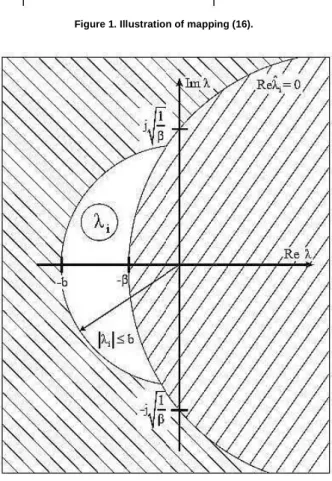
The half plane Reλˆ>>>>0is mapped by Eq. (16) into the λ

-plane in

the interior of the circle with the centre λ0====₂1(_α1−−−−β) α and the

radius r====₂1(_α1++++β)α assuming α > 0 according to Eq. (15). For

α

β 1

0<<<< <<<< the circle crosses the imaginary axis in the points

α β j

±±±± , cf. Fig. 1.

Obviously the stability behaviours of the original system (1) and the modified system represented by the matrices (14) do not agree. Only in the limit case of α → 0 , β → 0 , β /α → ∞ an agreement is

obtained.

2

β

α ==== small, ₂

b 1

<<<<

β (17)

are chosen where b is an upper bound of the eigenvalues

1 j ≤≤≤≤b,j====1,...,n

λ . (18)

Combining Eq. (16) and Eq. (18), the asymptotic stability of the modified system leads to the asymptotic stability of the original system (1) where the finite eigenvalues λj, j====1,...,n1, are located in a crescent-shaped region in the open left λ

-plane. An illustration of this case is represented in Fig. 2.

Figure 1. Illustration of mapping (16).

Figure 2. Stability region of system (1).

Modified Lyapunov Matrix Equation

Summarizing the results of section 3 the stability behaviour of (1) can be discussed by an inertia theorem of the modified Lyapunov matrix equation

Qˆ Aˆ Pˆ Eˆ Eˆ Pˆ

AˆT ++++ T ====−−−− . (19)

Theorem: If E⌢, Aˆ are defined by Eq. (14) with α , β according to

Eq. (17,18), then the descriptor system (1) is asymptotically stable if and only if for at least one symmetric, positive definite matrix

0 Qˆ

Qˆ ==== T >>>> (and then for all Qˆ ====QˆT>>>>0) there is a symmetric,

positive definite solution matrix Pˆ====PˆT>>>>0of Eq. (19).

The proof follows immediately from the standard Lyapunov

matrix equation for the system matrix AˆEˆ−−−−1or equivalently for Aˆ

Eˆ−−−−1 .

Remarks on the Eigenvalue Bound (18)

General Remarks

From state space discussions a theoretical eigenvalue bound b is known according to the slow subsystem (3):

1 A

b==== (20)

where each matrix norm can be applied. However, this bound again has the disadvantage that the transformationmatrices R , S (2) have to be known. The problem arises to find a bound b without knowing R , S .

This problem has been discussed by Müller (2004) recently. Still there is no general result with respect to the matrices E, A, but for the special case of semi-explicit systems with uniform index nice results have been found.

Semi-Explicit Systems with Uniform Index

Very often the descriptor system (1) is represented in semi-explicit form

) t ( x A ) t ( x A ) t (

xɺ1 ==== 11 1 ++++ 12 2 (21)

0====A₂₁x₁(t)++++A₂₂x₂(t) (22)

(Remark: Here the notation x1,x2is different to that of Eq. (3); in the following it will be referred to the new notation

of Eq. (21, 22) only.)

The index of a LTI descriptor system, which was mentioned with Eq. (2), indicates how often the algebraic equations (22) have to be differentiated to obtain ordinary differential equations for

((((

x (t) ...

))))

x2 ɺ2 ==== additionally. For one number less, k − 1 , the algebraic equations are solvable with respect to x2.

Each singular algebraic equation of the vector algebraic equation (22) may lead to an individual index. The utmost individual index represents the system index k . In the following it is assumed for simplicity of notation that the individual indices agree such that a uniform index is assumed. In the following the three cases of uniform indices k = 1 , k = 2 , k = 3 are considered.

Uniform Index 1

If system (21, 22) has index k = 1 then A₂₂is regular and

) t ( x A A ) t (

x2 ====−−−− 22−−−−1 21 1 (23)

((((

A A A A

))))

x(t) )

t (

xɺ₁ ==== ₁₁−−−− _{12 22}−−−−1 _{21 1} (24)

representing a state space system. This results immediately to the upper bound

λj ≤≤≤≤b==== A11−−−−A12A−−−−221A21 (25)

Uniform Index 2

Here A22and regularity of A21A12is assumed. Differentiating Eq. (22) leads to A21xɺ1(t)====A22(A11x1(t)++++A12x2(t))and

therefore ) t ( x A A ) A A ( ) t (

x2 ====−−−− 21 12 −−−−1 21 11 1 (26)

is obtained. Inserting Eq. (26) into Eq. (21) results in

) t ( x ] A A ) A A ( A A [ ) t (

xɺ₁ ==== ₁₁−−−− _{12 21 12} −−−−1 _{21 11 1} (27)

From here the upper bound

11 21 1 12 21 12 11

j≤≤≤≤b==== A −−−−A (A A )−−−−A A

λ (28)

is obtained.

Uniform Index 3

In this case the assumptions on system (21, 22) are

12 11 21 12

21

22 0, A A 0, A A A

A ==== ==== regular. Then

) t ( x A A ) A A A ( ) t (

x2 ====−−−− 21 11 12 −−−−1 21 112 1 (29)

holds resulting in the differential equation

) t ( x ] A A ) A A A ( A A [ ) t (

xɺ₁ ==== ₁₁−−−− _{12 21 11 12} −−−−1 _{21 11}2 ₁ (30)

The bound becomes

λj ≤≤≤≤b==== A11−−−−A12(A21A11A12)−−−−1A21A112 (31)

In this special cases eigenvalue bounds are available. But with increasing index the calculation becomes more and more expensive.

Example: Mechanical descriptor system with holonomic constraints

For example the mechanical descriptor system (4) with holonomic constraints (5) is considered. Then a semi-explicit representation (21, 22) is given by

; x ], q q [

x₁T==== T ɺT ₂====λ₁ (32)

0 A , 0 F A , F M 0 A , D M K M I 0 A 22 21 T 1 12 1 1 q 11 ==== ==== ====       −−−− −−−− ==== −−−− −−−− −−−− (33)

Assuming a regular mass matrix M and independent holonomic constraints, rankF====f , then it is easily shown that the mechanical descriptor system has uniform index k = 3:

T 1 12 11 21 12 21

22 0, A A 0, A A A FM F

A ==== ==== ==== −−−− (34)

According to Eq. (29) the constraint forces are determined by

[[[[

]]]]

      ==== −−−− −−−− −−−− −−−− ) t ( q ) t ( q D FM K FM ) F FM ( ) t

( 1 T 1 1 1

1

ɺ

λ (35)

System (30) runs as

) t ( x D K I 0 ) t ( x 1 q 1       −−−− −−−− ==== ɺ (36) with F ) F FM ( F M I P , D PM D , K PM

K==== −−−−1 ==== −−−−1 ==== q−−−− −−−−1 T −−−−1 T −−−−1 (37)

The upper eigenvalue bound (31) is given by

D K I 0 b q −−−− −−−− ==== (38)

In the case of symmetric matrices trices

T T T K K , D D , M

M==== ==== ==== this bound may be replaced by the

bound

((((

D8, K8

))))

max

b==== (39)

which follows by a discussion of the Rayleigh quotients according to a second order representation of Eq. (36). The index s characterizes the spectral norm.

Conclusions

It has been shown that for a matrix pencil

((((

λE−−−−A

))))

a modified

matrix pencil

((((

λEˆ−−−−Aˆ

))))

can be assigned such that the asymptotic stability of the new matrix pencil includes the asymptotic stability of the original pencil. The advantage of this modification consists in the regularity of the matrix ˆE and thus in the regularity of the modified Lyapunov matrix equation (19). The asymptotic stability can be guaranteed by the inertia theorem of section 4.

This result does not require any knowledge on the transformation matrices R , S for the Weierstrass-Kronecker representation (2) of the system, but it uses an upper bound (18) of the eigenvalues. This problem has been discussed in section 5 showing some first results but still simpler solutions are desired.

References

Dai, L., 1989, “Singular Control System”, Lecture Notes in Control and Information Sciences, Vol. 118, Berlin- Heidelberg, 332p.

Ishihara, J.Y. and Terra, M.H., 2002, “On the Lyapunov Theorem for Singular Systems”, IEEE Trans. Autom. Control, Vol. 47, pp. 1926-1930.

Lewis, F.L., 1986, “A Survey of Linear Singular Systems”, Circuits, Syst., Sig. Proc., Vol. 5, pp. 3-36.

Müller, P.C., 1993, “Stability of Linear Mechanical Systems with Holonomic Constraints”, Appl. Mech. Rev., Vol. 46, No. 11, Part 2, pp. S160-S164.

Müller, P.C., 2004, “Eigenvalue Bounds of Matrix Pencils”, PAAM-Proc. Appl. Math. Mech., Vol. 4, to appear.

Owens, D.H. and Debeljkovic, D.L., 1985, “Consistency and Lyapunov Stability of Linear Descriptor Systems: A

General Analysis”, IMA J. Math. Control & Inform., Vol. 2, pp. 139-151.

Stykel, T., 2002 a, “Stability and Inertia Theorems for Generalized Lyapunov Equations”, Linear Algebra and its Applications, Vol. 355, pp. 297-314.

Stykel, T., 2002 b, “On Criteria for Asymptotic Stability of Differential-Algebraic Equations”, Z. Angew. Math. Mech., Vol. 82, pp. 147-158.