Parsimonious Wavelet Kernel Extreme Learning Machine

(1)

Journal of Engineering Science and Technology Review 8 (5) (2015) 2129- 226

Research Article

Parsimonious Wavelet Kernel Extreme Learning Machine

Wang Qin1, Shen Yuantong2, Kuang Yu3, Wu Qiang4* and Sun Lin5

1_{Department of Information Technology, Hainan Medical University, Haikou 571101, China}

2

School of Mathematics and Physics, China University of Geosciences, Wuhan 430074, China 3

Department of Medical Physics, University of Nevada Las Vegas, Las Vegas, NV 89154, United States

4 _{Affiliated Hospital of Hainan Medical University, Haikou 571101, China}

5 _{Foreign Languages Department, Hainan Medical University, Haikou 571101, China}

Received 19 August 2015; Accepted 10 November 2015

___________________________________________________________________________________________

Abstract

In this study, a parsimonious scheme for wavelet kernel extreme learning machine (named PWKELM) was introduced by combining wavelet theory and a parsimonious algorithm into kernel extreme learning machine (KELM). In the wavelet analysis, bases that were localized in time and frequency to represent various signals effectively were used. Wavelet kernel extreme learning machine (WELM) maximized its capability to capture the essential features in “frequency-rich” signals. The proposed parsimonious algorithm also incorporated significant wavelet kernel functions via iteration in virtue of Householder matrix, thus producing a sparse solution that eased the computational burden and improved numerical stability. The experimental results achieved from the synthetic dataset and a gas furnace instance demonstrated that the proposed PWKELM is efficient and feasible in terms of improving generalization accuracy and real time performance.

Keywords:

Kernel extreme learning machine, Wavelet kernel function, Householder matrix, Sparse solution

__________________________________________________________________________________________

1. Introduction

The support vector machine (SVM) proposed by Vapnik solves quadratic regression problems with inequations [1]. Least squares support vector machine (LS-SVM) is a modified version of the standard SVM, and replaces the inequality constraints in addressing quadratic programming [2]. Thus, the training speed of LS-SVM is higher than that of SVM. Unfortunately, LS-SVM loses the sparseness of support vector, thereby degrading the generalization performance of SVM. In view of the sparseness of LS-SVM, a ﬁxed-size LS-SVM was proposed to realize the sparse representation in primal weight space [3]. Upon adding a bias term to the objective function, LS-SVM was solved through forward least squares approximation; thus, a sparse solution is generated in the least square sense [4]. Afterward,

a sparse algorithm of least squares support vector regression was established based on Householder transformation [5]. This algorithm can effectively sparsify the solution of LS-SVM.

The extreme learning machine(ELM) for single hidden-layer feedforward networks (SLFNs) has garnered significant interests among researchers since Huang et al.[6] first proposed their seminal work on ELM. In this machine, the input weights are chosen at random; the output weights can be analytically determined via the simple generalized inverse operation on the hidden layer output matrices. Empirical studies have indicated that the generalization

capability of ELM is comparable to or even better than that of SVMs and its variants [7].Thus, ELM has successfully been applied for classification [8] and regression [9].

Nonetheless, the number of hidden layer nodes, which is an important parameter of ELM, usually should be determined beforehand by users through some time-consuming methods. A special batch variant of ELM, namely, kernel extreme learning machine (KELM) [7], is proposed to avoid the problem of hidden nodes' selection. KELM transposes the explicit activation function into implicit kernel mapping. Unlike LS-SVM, KELM does not constrain Lagrange multipliers α_i ’s, therefore, LS-SVM generates a solution that is suboptimal to ELM. As with the conventional kernel methods, the core problem of KELM is the selection of kernel functions. In consideration of the nonstationary signals, an appropriate kernel function that can accurately capture the underlying information is expected to yield a compact representation. Commonly used kernel functions include Gauss function and polynomial function.

Wavelet analysis technology has recently been widely used to optimize neural networks. This technology is characterized by multiscale interpolation and the localization feature in both frequency and time domains. At present, wavelet kernel extreme learning machine (WKELM) has performed excellently in terms of classification [10].

In theory, the entire training sample in WKELM must be stored in the memory, which may generate redundant or unimportant wavelet kernel functions. A fundamental principle followed in system modeling is the well-recognized Occam’s razor hypothesis: “plurality should not be posited without necessity.” In other words, the simpler a solution is, the more reasonable it is. Sparse models are preferable in engineering applications because the

______________

J

estr

Engineering Science

and Technology Review

(2)

computational complexity of a model scales with its model complexity. Deng et al. recently proposed a reduced KELM (RKELM) that is capable of locating sparse topology by randomly selecting a subset from a training dataset [11]. However, numerical instability still exists. A fast sparse approximation scheme for KELM (FSA-KELM) [12] was recently introduced to obtain a simple sparse solution; this process begins with a null solution and gradually selects a new hidden node according to some criteria. This procedure is repeated until the stopping criterion is met.

In the current study, a parsimonious algorithm and wavelet technique are developed for KELM on the basis of the aforementioned analysis, the resultant model is referred to as parsimonious wavelet kernel extreme learning machine (PWKELM). Wavelet function benefits from multiscale interpolation and is also suitable for the local analysis and detection of transient signals. As a result, a wavelet expansion representation is compact and is easy to implement. Householder matrix is also used to orthogonalize the linear equation set in WKELM, and significant wavelet kernel functions are recruited iteratively. Thus, a sparse solution is established. Synthetic and real-world data sets are utilized in conducting experiments whose results confirm the effectiveness and feasibility of the proposed PWKELM.

The rest of this paper is organized as follows: ELM and WKELM are introduced in Section 2. The PWKELM algorithm and its detailed procedure are listed as well. The experimental results and analyses are presented in Section 3. Conclusions follow in the final section.

2. Methodology

2.1 ELM

ELM is based on the perceptron model with a single hidden-layer and has a simple three hidden-layer structure. This structure is composed of the input, output, and hidden layers. If we randomly assign the input weights and bias values, we need not to adjust the input weights or hidden layer bias throughout the learning process.

For N training samples

{

(

xi,ti

)

}

_i =1

N ,x

i∈!

n

,t_i_∈_!, the

SLFN model with _N! _{hidden nodes (additive or RBF nodes)} can be formulated as

β_ig w

i,bi,xj

(

)

i=1

!

N

∑

=o_j,j=1,",N (1)

where βi is the output weight connected to the ith hidden

layer node, w

i and bi are learning parameters of hidden

layer nodes,o_j∈! is the output of ELM, and g

( )

i _{is the}

activation function. Eq. (1) can be written compactly as

Hβ=o ₍₂₎

where

o =[o

1,!,oN] T

,β=[β₁,!_,_β_" N]

T ,

H=

g w

1⋅x1+b1

(

)

!_g

(

w_N"⋅x₁+b_N"

)

#!#

g w

1⋅xN+b1

(

)

!_g

(

w_N"⋅x_N+b_N"

)

⎡

⎣ ⎢ ⎢ ⎢ ⎢

⎤

⎦ ⎥ ⎥ ⎥ ⎥_N×_N"

.

H is called the output matrix of the hidden layer. If the ELM model with N! _{hidden nodes can approximate}_N samples with zero error, then it means that there exist βi

such that

β_iG w

i,bi,xj

(

)

i=1

!

N

∑

=t_j,j=1,",N

(3)

where t_j is the target value. Eq. (3) can be expressed in the

following matrix-vector form

Hβ=T (4)

where T= t

1,t2,!,tN

⎡⎣ ⎤⎦T

. The hidden nodes’ learning

parameters w

i and bi are randomly generated in the beginning. Thus Eq. (4) then becomes a linear system and the output weights β can be computed analytically by finding the minimum norm least squares’ solution as follows

β=_H†

T (5)

where _H†

is the Moore-Penrose generalized inverse of _H_.

2.2 WKELM

The universal approximation capability of ELM with hidden nodes has been proven. KELM is proposed in response to the problem of selecting the demanding hidden nodes. KELM substitutes the kernel function mapping for the hidden layer mappingh x

( )

_.

Given a training set x_i,t i

(

)

{

}i

=1

N

,x_i_∈!n,t

i∈! , the original optimization problem of KELM can be expressed as

min L

ELM =

1 2||β||

2

+C

2ξi 2

s_.t_.h x i

( )

β=t

i−ξi, i=1,!,N

(6)

The corresponding Lagrangian dual problem can be formatted as

L ELM=

1 2||β||

2 +C

2 ξi

2

i=1 N

∑

− αi

(

h x

( )

i β −ti+ξi

)

i=1

N

∑

(7)

The KKT optimality conditions of Eq. (7) are as follows

β=HT_α

(8)

I

C

+_HHT

⎛ ⎝⎜

⎞ ⎠⎟α=T

(9)

The feature mapping h x

( )

_{can be unknown, but the}

corresponding kernel is usually given, the kernel matrix of ELM can be deﬁned as follow

K

ELM=HH

T :K

(3)

Consequently, the output function of KELM can be written as

f

( )=

x h x

( )

HT I C+

HHT ⎛ ⎝⎜

⎞ ⎠⎟ −1

T

=

k x, x

1

(

)

M k

(

x, x_N

)

⎡

⎣ ⎢ ⎢ ⎢ ⎢

⎤

⎦ ⎥ ⎥ ⎥ ⎥ T

I

C+KELM

⎛ ⎝⎜

⎞ ⎠⎟ −1

T

(11)

The wavelet is a ﬁnite-length waveform that is characterized as follows: (1) either time domain or approximation is compactly supported; And (2) the advantages of wavelet analysis are integrated into the time and frequency domains. The time domain characteristics of wavelet transform can be expressed with wavelet functions that are translated from a wavelet kernel function. Meanwhile, we apply different wavelet functions to approximate the original signals. Wavelet analysis is a relatively new signal processing tool that is widely applied by many researchers in power systems due to its excellent characteristics. Thus, the combination of the wavelet analysis technique and KELM is significant.

If a function satisﬁes the Mercer theorem, then it is a kernel function. The function can also be used as a kernel function of the KELM. Many wavelet functions satisfy the translation-invariant kernel conditions, including the Mexican hat wavelet kernel function [13]. In this study, WKELM is utilized for regression.

2.3 PWKELM

Given a wavelet kernel function k

(

x, y

)

, the function

k

(

x, xi

)

corresponds to a wavelet kernel function for each

training sample x

i . A set of wavelet kernel functions V=

{

k

|i_∈Q

{

}

according to some criteria by starting with an empty index set S=∅ and a full index setQ=

{

1,!,N

}

.

Then, the index p is removed fromQand added to S. At

the

(

n₋₁

)

_{th iteration, the number of wavelet kernel}

functions in the set

{

k

(

x, x_i

)

|i_∈S

}

_{is presumably}_n₋₁_{. Eq.}

(9) is rearranged as

KSαS

*₍n−₁₎

=T (12)

where

K

S=⎣⎡ki,!,kj⎤⎦

(

i,j∈S

)

with _k

i=ki+ei/C , _k

i is the

i th column vector of _K , and α S

∗₍n−₁₎ is a subvector

consisting of elements that are confined to the index set S at the _n

−1

(

)

th iteration. Eq. (12) is an overdetermined linear

equation set; its solution is simply equivalent to finding the optimal solution to the following problem

min

α S

n−1

( ) GS n−₁ ( )

= KSα

S n−₁ ( )₋

T

{

}

(13)

The optimal solution of Eq. (13) can be analytically determined as follows

α S

∗₍n−₁₎

= KS T

KS

(

)

−₁

KS T

T (14) Thus, we can get the minimizer of (13) with

G

S ∗₍n−₁₎

= KSαS ∗₍n−₁₎

−_T (15)

Eq. (13) indicates that the larger the _G S

∗₍n₋₁₎ value is, the

worse the approximate effectiveness becomes. If

k

(

x, x_p

)

is

recruited as the new wavelet kernel function at the nth

iteration, then

G_S∪{ }p

∗( )n can be obtained by following by the

similar lines

G_S∗_∪( )n_{{ }}_p = K

Skp

⎡ ⎣ ⎤⎦

α

S ∗( )n

α

p ∗

⎡

⎣ ⎢ ⎢

⎤

⎦ ⎥ ⎥−T

(16)

Consequently, G_S∪{ }p

∗( )n _≤

G_S∗(n−1), andΔG_p( )n ≥0. Thus, the

criterion of recruiting the next wavelet kernel function at the

nth iteration is obtained as follows

p=arg max

i∈Q ΔGi n

( )

(17)

where

Q=

{

1,…_,_N

}

_\_S . Eq. (17) indicates that at each

iteration, the wavelet kernel function introducing the most significant decrease on _G is recruited as the new kernel function. Eq. (13) can be solved by using Eq. (14) to calculate _G and _ΔG at each iteration. The use of Eq. (14)

incurs two potential risks: on the one hand, the reliability and robustness of calculating

KS T

KS

(

)

−1 is closely related to

its condition number, defined as

κ KS T

KS

(

)

=_κ2

KS

( )

=µmax

2

µmin 2

(18)

where µmax

and

µ_min represent the maximum and minimum

nonzero singular values of KS

, respectively. In general, the

larger the condition number is, the less stable the numerically calculating result is. The condition number easily incurs roundoff errors if it is excessively large. On the other hand, the recursive strategy is more difficult to use for recruiting new wavelet kernel function at the nth iteration.

(4)

Based on knowledge regrading matrix transformation, matrix

KS

can be decomposed as

KS=QN×N n−1

( ) R(n−1)×(n−1)

n−1

( )

0

N+1−n

( )×(n−1)

⎡ ⎣ ⎢ ⎢ ⎤ ⎦ ⎥ ⎥

through QR decomposition [14]. In

the present study, QN!N

n₋₁

( ) is an orthogonal matrix that

satisfies QN_×N

n₋₁

( )

(

)

T

QN_×N n₋₁

( )

=QN_×N n₋₁

( ) _Q

N_×N n₋₁

( )

(

)

T and

R(n−1)×(n−1) n₋₁

( ) is an

upper triangular matrix with the same rank as _KS. Thus,

G

S n−1

( ) = KSαS

n−1

( )₋_T = QN×N

n−1

( )

(

)

T

KSαS n−1

( )₋ QN×N

n−1

( )

(

)

T

=

R₍n−₁₎×₍n−₁₎

n−1

( )

0

N₊₁−n

( )×(n−1) ⎡ ⎣ ⎢ ⎢ ⎤ ⎦ ⎥ ⎥αS

n−1

( )₋ ⌢

T

n−1

( )×1 n−1

( )

"

T

N−n₊₁

( )×1 n−1

( ) ⎡ ⎣ ⎢ ⎢ ⎢ ⎤ ⎦ ⎥ ⎥ ⎥ ⎧ ⎨ ⎪ ⎩ ⎪ ⎫ ⎬ ⎪ ⎭ ⎪

= R(n−1)×(n−1)

n−1

( ) _α

S n−1

( )₋_T⌢

n×1 n−1

( )

+ T"

N−n₊₁

( )×1 n−1

( )

(19)

Given that !

T(N₋n₊₁)_×₁ n₋₁

( ) _{is constant, the matrix is an upper}

triangular matrix and α

S

∗(n−₁)

can easily be obtained by solving

R₍n−₁₎×₍n−₁₎ n−₁

( ) _α

S n−₁ ( )

=T⌢n×₁ n−₁

( ) ₍₂₀₎

For Eq. (14), κ KS T

KS

(

)

=µmax

2

/µmin 2

; however,

κ R₍n₋1₎×₍n₋1₎

n₋1 ( )

(

)

=_κ _K

S

( )

=µ_max/µ_min in Eq. (20). Generally, κ>1, which indicates that the optimal solution of Eq. (13) derived from Eq. (20) is more stable numerically than that from Eq. (14). In addition,

G

S

∗₍n₋₁₎

=T!₍N₋n₊₁_)×1 n₋₁

( ) ₍₂₁₎

In the following iteration, if k

(

x, x_p

)

is recruited as the

new wavelet kernel function, thenG_S∪{ }p

∗( )n _{is obtained through}

a lower-cost strategy rather than from scratch through Eq. (19).

Let

(

Q(n−1)

)

T

⌢ K_n−

1 ( )×₍N−n+1₎

n−1

( )

" K

N+1−n ( )×₍N−n+1₎

n−1 ( ) ⎡ ⎣ ⎢ ⎢ ⎢ ⎤ ⎦ ⎥ ⎥ ⎥

=K_Q. Householder matrix

[15] is applied as follows

G_S( )n_∪_{{ }}_p=

I₍_n₋₁₎_×₍_n₋₁₎ 0 0 H_p( )n

⎡ ⎣ ⎢ ⎢ ⎤ ⎦ ⎥ ⎥ QN×N

n−1 ( )

(

)

T

K_Sk_p

⎡⎣ ⎤⎦ αS

n ( ) αp ⎡ ⎣ ⎢ ⎢ ⎤ ⎦ ⎥ ⎥−T ⎛ ⎝ ⎜ ⎜ ⎞ ⎠ ⎟ ⎟ =

I₍_n₋₁₎_×₍_n₋₁₎ 0 0 H_p( )n

⎡ ⎣ ⎢ ⎢ ⎤ ⎦ ⎥ ⎥

R₍(_nn₋−₁1₎)_×₍_n₋₁₎ k⌢_p(n−1) 0

N+1−n ( )×(n−1)k"p

n−1 ( ) ⎡ ⎣ ⎢ ⎢ ⎢ ⎤ ⎦ ⎥ ⎥ ⎥ αS n ( ) αp ⎡ ⎣ ⎢ ⎢ ⎤ ⎦ ⎥ ⎥− ⌢ T

n−1 ( )×1

n−1 ( )

" T

N−n+1 ( )×1

n−1 ( ) ⎡ ⎣ ⎢ ⎢ ⎢ ⎤ ⎦ ⎥ ⎥ ⎥ ⎛ ⎝ ⎜ ⎜ ⎞ ⎠ ⎟ ⎟ =

R₍(_nn₋−₁1₎)_×₍_n₋₁₎ k⌢_p(n−1)

0

1×(n−1) −sign k"p n−1 ( )

(

)

1

"

k_p(n−1)

0 N−n

( )×(n−1) 0(N−n)×1

⎡ ⎣ ⎢ ⎢ ⎢ ⎢ ⎢ ⎤ ⎦ ⎥ ⎥ ⎥ ⎥ ⎥ αS n ( ) αp ⎡ ⎣ ⎢ ⎢ ⎤ ⎦ ⎥ ⎥− ⌢ T

n−1 ( )×1

n−1 ( )

⌢ T_p( )n

" T

N−n ( )×1

n ( ) ⎡ ⎣ ⎢ ⎢ ⎢ ⎢ ⎢ ⎤ ⎦ ⎥ ⎥ ⎥ ⎥ ⎥ ⎛ ⎝ ⎜ ⎜ ⎜ ⎜ ⎜ ⎞ ⎠ ⎟ ⎟ ⎟ ⎟ ⎟ =

R₍(_nn₋−₁1₎)_×₍_n₋₁₎ k⌢_p(n−1)

0

1×(n−1) −sign k"p n−1 ( )

(

)

₁ k"_p(n−1)

⎡ ⎣ ⎢ ⎢ ⎢ ⎤ ⎦ ⎥ ⎥ ⎥ αS n ( ) αp ⎡ ⎣ ⎢ ⎢ ⎤ ⎦ ⎥ ⎥− ⌢ T

n−1 ( )×1

n−1 ( )

⌢ T_p( )n

⎡ ⎣ ⎢ ⎢ ⎤ ⎦ ⎥ ⎥ ⎛ ⎝ ⎜ ⎜ ⎜ ⎞ ⎠ ⎟ ⎟ ⎟

+ T" N−n ( )×1

n ( )

(

22)

where k⌢

p n−1

( ) _and _k! p

n−1

( ) _{are derived from} ⌢

K₍n₋₁_)×₍N₋n₊₁₎ n₋₁

( ) _and

!

K(N+1−n)_×(N₋n₊₁) n₋₁

( ) _{corresponding to the index} p.Hp

n

( )_{is derived}

as

H p

n ( )

==I₋₂

v p

n ( ) _v

p n ( )

( )

T

v p

n ( )

( )

T

v p

n

( ) (23)

where

v p

n

( ) =k!

p n-1

( )

+sign( k! p

n-1

( )

(

)

1 ) k!

p n-1

( ) _e

1 (24)

Rn×n n

( )_{, together with}⌢ Tn"1

n−1

( )_{, is updated as}

R n×n n ( ) = R n−1

( )×(n−1)

n−1 ( ) k⌢ p n−1 ( ) 0

1×₍n−1₎ −sign k"p n−1

( )

(

)

1

" k p n−1 ( ) ⎡ ⎣ ⎢ ⎢ ⎢ ⎤ ⎦ ⎥ ⎥ ⎥

，_Tn×⌢ 1 n

( )

=

⌢

T(_n−1)×1 n−1 ( ) ⌢ Tp n ( ) ⎡ ⎣ ⎢ ⎢ ⎤ ⎦ ⎥ ⎥ (25)

Thus, the optimal solution at the n th iteration is determined with

R n−1 ( )×(n−1)

n−1 ( ) _k⌢

p n−1 ( )

0

1×(n−1) −sign k"p n−1 ( )

(

)

1 " k p n−1 ( ) ⎡ ⎣ ⎢ ⎢ ⎢ ⎤ ⎦ ⎥ ⎥ ⎥ α S n ( ) α p ⎡ ⎣ ⎢ ⎢ ⎤ ⎦ ⎥ ⎥= ⌢ T n−1 ( )×1

n−1 ( )

⌢ T_p( )n ⎡ ⎣ ⎢ ⎢ ⎤ ⎦ ⎥

⎥ (26)

The following is obtained as well

G_S∪{ }p

∗( )n

= T!(N−n)×1 n

(5)

Hence, according to Eqs. (21) , (22), and (27), the following is obtained

ΔG_p( )n = _T!_N −n+1

( )×1 n−1

( )

− T!(N−n)×1

n

( )

= Hp n

( )_! T(N−n+1)×1

n−1

( )

− T!(N−n)×1

n

( )

=T⌢p n

( ) (28)

The criterion considered in recruiting the next wavelet kernel function is

p=arg max i∈Q

⌢

T_i( )n (29)

According to Eq. (22), T⌢p n

( )_{is easily gained explicitly as}

⌢ Ti n

( ) = H

p n

( )_" T(N−n+1)×1

n−1 ( )

(

)

₁

= T"(N−n+1)×1

n−1 ( )

(

)

₁−2

v

i n

( )

₁ v

i n

( )

T

" T(N−n+1)×1

n−1 ( )

v

i n

( )

T

v

i n

( )

(30)

where

( )

⋅₁represents the extraction of the first element of a

given column vector. Hp n

( )_{should be constructed when the}

new wavelet kernel function k

(

x, x_p

)

is determined;

subsequently, Eq. (25) and the index setsS←_S∪

{ }

_p _{, and}

Q←_Q\

{ }

p are updated. Then, K⌢_{( )×}n ₍N₋n₋₁₎ n

( ) _and !

K₍N₋n_)×₍N₋n₋₁₎ n

( )

can be refreshed as

⌢ K

n

( )×(N−n) n

( )

" K

N−n

( )×(N−n) n−1 ( ) ⎡

⎣ ⎢ ⎢ ⎢

⎤

⎦ ⎥ ⎥ ⎥

=

I₍_n₋₁₎_×₍_n₋₁₎ 0 0 H

p n

( ) ⎡

⎣ ⎢ ⎢

⎤

⎦ ⎥ ⎥

⌢ K

n−1 ( )×₍N−n+1₎

n−1

( ) _\_k⌢

p n−1 ( )

" K

N+1−n

( )×₍N−n+1₎

n−1

( ) _\_k_"

p n−1 ( ) ⎡

⎣ ⎢ ⎢ ⎢

⎤

⎦ ⎥ ⎥ ⎥

(31)

In this study, the value of index nstarts from 1. Thus, we must first initialize PWKELM. Let

ki=Qiri

(

i=1,!,N

)

(31)

where k

i is obtained from K=KELM+I/C that corresponds

to the index i. Q_i is obtained via QR decomposition.

According to Eq. (19), Ti!( )0 is derived as

!

Ti

0

( )₌

Q_iT\_T⌢ i

0

( ) ₍₃₂₎

Thus, the first wavelet kernel function is selected as follows

p=arg min

i∈Q !

Ti( )0 (33)

In summary, the flowchart of PWKELM is depicted as follows

Step 1) Initializations

Obtain the training data set x_i,t i

(

)

{

}i

=1 N

.

Choose the appropriate regularization and wavelet kernel parameters.

Let S=∅ and Q=

{

1,!,N

}

, n=1.

Calculate !

Ti

0

( )_{according to (32).}

Recruit the first k

(

x, x_p

)

according to (33).

Let S←S∪

{ }

p ,Q←Q\

{ }

p , n=2.

Let H( )1=Q_p _,_R( )1=

( )

rp

1, calculate ⌢

K1×N 1

( ) _and ! K₍N₋₁_)×N

1 ( )

via

⌢

K1×N( )1

"

K₍N−1₎×N 1 ( )

⎡

⎣ ⎢ ⎢

⎤

⎦ ⎥

⎥=H

1 ( )

KELM+I/C

(

)

, compute

⌢

T1×1 1

( )_and! T(N₋₁)×1

1

( ) _{according to} ⌢

T1×1 1 ( )

"

T(N−1)×1 1 ( ) ⎡

⎣ ⎢ ⎢

⎤

⎦ ⎥ ⎥=H

1 ( )

T.

Choose a positive M or a small ε_>0_.

Step 2) If n>M or ⌢

T

p i

( )

2

i=0

n

∑

T <ε Step 3) Go to step 11

Step 4) Else

Step 5) Calculate v

i n

( )_and⌢

Ti( )n according to (24) and (30) respectively.

Step 6) Choose the next k

(

x, x_p

)

according to (29).

Step 7) Update R( )n and T⌢( )n according to (25).

Step 8) Update K⌢( )×n (N₋n) n

( ) _and !

K(N₋n)×(N₋n) n

( ) _{according to (31).}

Step 9) Let S←_S∪

{ }

_p _,_Q←_Q\

{ }

p , n=n+1, go to step

2.

Step 10) End if

Step 11) Solve R( )nα S

n ( )

=Tn×⌢ 1

n ( )_.

Step 12) Output f x

( )

=

k

(

x, xi

)

M

k

(

x, x_l

)

⎡

⎣ ⎢ ⎢ ⎢ ⎢

⎤

⎦ ⎥ ⎥ ⎥ ⎥₍_i,!,l∈_S₎

T

α S

n

( ) .

3. Result Analysis and Discussion

(6)

3.1Single-variable synthetic data

In this experiment, we approximate the following single-variable function

f x

20,30,!,150

{

}

×

{

0.01,0.02,!,0.2

}

via cross validation. WELM is compared with ELM, LS-SVM and ELM with RBF kernel. The experimental precisions are presented in Table 1. The time requirement of WKELM is comparable with those of ELM and RBF KELM but is slightly shorter than that of the RBF LS-SVM. The accuracy of WKELM, which is comparable with other algorithms on training samples, is the highest on testing samples. Wavelet kernel function can match well the original series on different scales. The generalization capability of ELM is clearly comparable with or is even better than LS-SVM.

Tab. 1. Comparison of different algorithms Algorithm Parameters

C,σ2

(

)

Times (s) Training Testing

Training Testing RMSE RMSE

WKELM

₍

_60,0.04

₎

0.0335 0.0094 0.0896 0.0124

RBF

KELM

(

100,0.03

)

0.0336 0.0089 0.0895 0.0141

ELM _ 0.0287 0.0134 0.0893 0.0159

RBF

LS-SVM

(

70,0.04

)

0.0381 0.0125 0.0900 0.0164

Figs.1 to 3 illustrate the experimental results for different sparse algorithms given only 10 wavelet kernel functions. PWKELMwith only 10 wavelet kernel functions can attain an excellent generalization performance similar to WKELM, but RKELM and FSA-ELM lose approximation capability to some extent. On the premise of the same sparsity ratio of kernel functions, PWKELM proves to be superior in regression accuracy to RKELM and FSA-ELM, that is, new kernel functions must be recruited for other sparse algorithms to achieve the same generalization performance as PWKELM. Therefore, PWKELM obtains the best sparseness among these algorithms; this finding signifies that PWKELM can enhance computational efficiency in the testing phase, thereby improving its real time performance. With regard to computational stability, roundoff errors and numerical instability are easily incurred by calculating α

S n ( )

with KST KS

(

)

−1

directly in RKELM, but Householder matrix

introduced in this study eliminates the bottleneck.

0 0.2 0.4 0.6 0.8 1

-1.5 -1 -0.5 0 0.5 1 1.5 2

x y

Training data PWKELM

Sparse Wavelet kernel functions WELMK

Fig.1. Simulation results of PWKELM

0 0.2 0.4 0.6 0.8 1

-1.5 -1 -0.5 0 0.5 1 1.5 2

x y

Training data RKELM

Sparse Wavelet kernel functions WELMK

Fig.2. Simulation results of RKELM

0 0.2 0.4 0.6 0.8 1

-1.5 -1 -0.5 0 0.5 1 1.5 2

x y

Training data FSA-KELM

Sparse Wavelet kernel kernels WELMK

Fig.3. Simulation results of FSA-ELM

3.2 Gas furnace example

The gas furnace data set is a time series containing 296 pairs of input-output points as depicted in Fig. 3, where the input

v

k is the coded input gas feed rate and the output yk represents the CO2 concentration from the gas furnace [16].

A total of 293 new data points x k,yk

(

)

{

}

are derived from these pairs and constructed with x

k given as

x

k=⎡⎣yk-1,yk-2,yk-3,vk-1, vk-2,vk-3⎤⎦ T

(7)

Fig. 3 indicates that the gas furnace sample series

ﬂuctuates sharply, and the rear part is different from the front. Hence, the even-number pairs of x

k,yk

(

)

{

}

are used for training, whereas the odd-numbered pairs for testing. As a result, the training sets contain 146 data points, while the training sets have 147. The optimal regularization and kernel

parameters are derived from the set

{

2-5_,2-4_,_…_,215

}

using

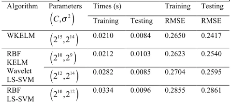
cross validation, and the experimental results are presented in Table 2. Fig.4 exhibits the tendency of the performance index RMSE against the number of wavelet kernel functions.

0 50 100 150 200 250 300

-3 -2 -1 0 1 2 3

sy

st

em

i

n

p

u

t

sample

(a)

0 50 100 150 200 250 300

44 46 48 50 52 54 56 58 60 62

sample

sy

st

em

o

u

tp

u

t

(b)

Fig. 3. Gas furnace: (a) input v

k and (b) output yk.

Tabla 2. Comparison of different kernels Algorithm Parameters

C,σ2

the number of wavelet basis functions

RM

S

E

WKELM PWKELM FSA-ELM RELM

Fig.4. RMSE vs.the number of wavelet kernel functions on gas furnace instance

Table 2 implies that WKELM is relatively more accurate in prediction and efficient in calculating. ELM usually reports a generalization performance on regression that is superior to that of LS-SVM. WKELM gains advantages in different wavelet functions that approximate the details of numerous series. Fig4 illustrates that RMSE decreases with an increase in the number of wavelet kernel functions for every algorithm. The dashed line generated by WKELM is regarded as the benchmark line; the other results are terminated when they reach this line. PWKELM reaches the benchmark line first, which suggests that PWKELM requires the least number of wavelet kernel functions to attain almost the same generalization performance compared with the other sparse algorithms do. That is, the use of PWKELM serves to provide WKELM with a much sparser solution without sacrificing the generalization performance. The testing time is directly proportional to the number of kernel functions; thus, a sparser solution indicates the less testing time. A decreased testing time suggests improved real time performance. In sum, the experiment based on a gas furnace example demonstrates the feasibility and efﬁcacy of the proposed PWKELM.

4. Conclusions

(8)

as RKELM and FSA-ELM, in terms of the number of wavelet kernel functions under nearly the same generalization performance. That is to say, PWKELM is able to generate a more parsimonious WKELM without impairing the generalization and identification accuracy. This outcome is paramount for the environments strictly

demanding the computational efficiency in engineering applications.

Acknowledgements

The study was supported by the National Natural Science Foundation of China (Grant Nos. 11301120).

______________________________

References

1. Vapnik V. N., “The Nature of Statistical Learning Theory”. New York: Springer-Verlag, 1995.

2. Suykens J. A. K., Vandewalle J., “Least squares support vector machine classifiers”. Neural Processing Letters, 9(3), 1999, pp.293– 300.

3. Mall R., Suykens J.A.K., “Sparse reductions for ﬁxed-size least squares support vector machines on large scale”. Advances in Knowledge Discovery and Data Mining. Lecture Notes in Computer Science, 2013, pp.161–173.

4. Xia X. L., Jiao W., Li K., Irwin G., “A novel sparse least squares support vector machines”. Mathematical Problems in Engineering, 2013(1), 2013, pp.681-703.

5. Zhao Y. P., Li B., Li Y. B., Wang K. K., “Householder transformation based sparse least squares support vector regression”.

Neurocomputing, 161, 2015, pp.243-253.

6. Huang G. B., Zhu Q. Y., Siew C. K., “Extreme learning machine: Theory and applications”. Neurocomputing, 70(1), 2006, pp.489-501. 7. Huang G. B., Zhou H., Ding X., Zhang R., “Extreme learning machine for regression and multiclass classiﬁcation”. IEEE

Transactions on Systems, Man and Cybernetics part B, Cybernetics, 42

(2), 2012, pp.513-529.

8. Man Z., Lee K., Wang D., Cao Z., Khoo S., “Robust single-hidden layer feedforward network-based pattern classiﬁer”. IEEE Transactions on Neural Networks & Learning Systems, 23(12), 2012, pp.1974-1986.

9. Grigorievskiy A., Miche Y., Ventelä A. M., Séverin E., Lendasse A., “Long-term time series prediction using OP-ELM”. Neural Networks, 51(3), 2014, pp.50-56.

10. Wang J., Guo C. L., “Wavelet kernel extreme learning classiﬁer”. Microelectron &Computer, 10, 2013, pp.73-76+80.

11. Deng W. Y., Zheng Q. H., Zhang K., “Reduced kernel extreme learning machine”. Proceedings of the 8th International Conference on

Computer Recognition Systems CORES 2013, Milkow, Poland: Springer

International Publishing, 2013, pp.63-69.

12. Li X. D., Mao W. J, Jiang W., “Fast sparse approximation of extreme learning machine”. Neurocomputing, 128(5), 2014, pp.96-103 13. Ding S. F., Wu F. L., Shi Z. Z., “Wavelet twin support vector machine”. Neural Computing & Applications, 25(6), 2014, pp.1241-1247.

14. Zhang X., “Matrix Analysis and Applications”.Tsinghua University Press, Beijing, China, 2004.

15. Dubrulle A. A., “Householder transformations revisited”. Siam Journal on Matrix Analysis & Applications, 22(1), 2000, pp.33-40. 16. S. Chen, X. Hong, C. J. Harris. “Particle swarm optimization aided orthogonal forward regression for uniﬁed data modeling”. IEEE