Two-phase deformations within the
framework of phase transition zones
A.B. Freidin, E.N. Vilchevskaya, L.L. Sharipova
∗ Issues dedicated to memory of the Professor Rastko Stojanovi´cAbstract
We analyze conditions on the equilibrium interface and de-velop the concept of phase transition zones (PTZ) formed in strain-space by all deformations which can exist on the equilib-rium interface. The importance of the PTZ construction follows from the fact that deformations outside the PTZ cannot exist on the interface, whatever the loading conditions. The PTZ bound-ary acts as a phase diagram or yield surface in strain-space. We develop a general procedure for the PTZ construction and give examples for various nonlinear elastic materials and in a case of small strains. We study orientations of the interface and jumps of strains on the interface and demonstrate that various points of the PTZ correspond to different types of strain localization due to phase transformations on different loading path.
1
Introduction
From the mechanical point of view phase transitions in deformable solids result in the appearance of strain fields with interfaces which are the surfaces of discontinuity in deformation gradient at continuous displacements [10, 12, 11]. We analyze conditions on the equilibrium interface and develop the concept of phase transition zones (PTZ). The PTZ is formed in strain-space by all deformations which can exist on ∗Institute of Mechanical Engineering Problems, Russian Academy of Sciences,
St. Petersburg, Russia (e-mail: [email protected])
the equilibrium interface. The PTZ is determined entirely by properties of the strain energy function of a material. The importance of the PTZ construction follows from the fact that deformations outside the PTZ cannot exist on the interface, whatever the loading conditions. The PTZ boundary acts as a phase diagram or yield surface in strain-space. We describe a general procedure for the PTZ construction [4, 5] and give examples for various nonlinear elastic materials. Then we develop a small strain approach to the theory of phase transitions in elastic solids. The problem is reduced to the analysis of the linear elastic-ity equations for heterogeneous medium with an additional condition of phase equilibrium on the interface. The thermodynamic condition takes the form of an equation that determines the normal to the inter-face in dependence on a tensor that acts as a dislocation momentum tensor induced by new phase areas.
Since the PTZ occurs naturally in the analysis of the local equi-librium conditions, any point of the PTZ can be associated with some piece-wise linear two-phase deformations. We study characteristic fea-tures of such deformations – orientation of the interface and the jump of strains. As a result we demonstrate that different passes of de-formation lead to different types of strain localization due to phase transformations.
2
Preliminaries. Equilibrium phase
boundaries and phase transition
zones
We are interested in equilibrium deformation fields such that the dis-placements are twice differentiable everywhere in a body besides a con-tinuously differentiable surfaces (interfaces) at which the deformation gradient suffers a jump at continuous displacement.
equilibrium interface:
[[F]] =f ⊗m, (2.1)
[[S]]m= 0, (2.2)
[[W]] =f ·S±m, (2.3)
whereFis the deformation gradient,W is the strain energy per unit ref-erence volume (the elastic potential),S=WF(F) is the Piola stress
ten-sor related with Cauchy stress tenten-sor as T =J−1SFT, J = det F> 0, brackets [[·]] = (·)+ −(·)− denote the jump of a function across Γ,
super- or subscripts “−” and “+” identify the values on different sides of the shock surface.
The kinematic condition (2.1) follows from the continuity of the displacement [20]. The vector f = [[F]]m is called the amplitude. The traction continuity condition (2.2) follows from equilibrium considera-tions.
An additional thermodynamic condition (2.3) [10, 12, 19, 11, 2, 18] arises from an additional degree of freedom produced by free phase boundaries. One could also see (2.3) in [14].
By (2.1), the conditions (2.2) and (2.3) can be rewritten as (S(F+f ⊗m)−S(F))m= 0,
W(F+f ⊗m)−W(F) =f ·S(F)m
where F ≡ F−. Given F, the above equations can be considered as a
system of four equations for five unknowns: the amplitude f 6= 0 and the unit normal m. Those F only for which the system of equations can be solved can be on the interface.
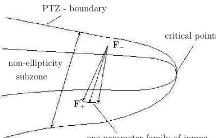
Definition [4]. The phase transition zone is formed by all defor-mations which can exist on a locally equilibrium phase boundary.
For thoseFinside the PTZ, there in general exists an one-parameter family of solutions for f and m.
critical points F−
F+
one-parameter family of jumps PTZ - boundary
non-ellipticity subzone
Figure 1: Phase transition zone in strain space.
interface then a material must be non-elliptic at some segment on the path
F(ξ) =F−+ξf ⊗m (ξ∈(0,1))
Thus, the PTZ contains the non-ellipticity sub-zone.
3
Phase transition zones for isotropic
nonlinear elastic materials
The conditions (2.1), (2.2), (2.3) can be rewritten as
F± = (I+a∓⊗n)F∓, (3.1)
[[T]]n= 0, (3.2)
[[W]] = c·Tn (3.3)
whereIdenotes the unit tensor,n is the normal to the interface in the deformed configuration,
n=|F−∓Tm|−1F−∓Tm, m=|FT∓n|−1FT∓n. (3.4) Amplitudes f, a∓ and c are related as
c,JN1−1/2f =J−a−=J+a+, (3.5)
where N1∓ = |FT∓n|2 = n·B∓n, B = FFT is the left Cauchy-Green
tensor, and, as can be shown [4], [[JN1−1/2]] = 0. In a case of nonlinear elastic isotropic materials
W =W(I1, I2, J), T=µ0I+µ1B+µ−1B−1, (3.6)
µ0 =W3+ 2J−1I2W2, µ1 = 2J−1W1, µ−1 =−2JW2, (3.7)
where
I1 =λ21+λ22+λ23 = trB,
I2 =λ21λ22+λ21λ32+λ22λ23 =J2trB−1,
J =λ1λ2λ3
(3.8)
are the strain invariants, λi >0 (i= 1,2,3) are the principal stretches,
W1, W2, W3 denote∂W/∂I1, ∂W/∂I2 and ∂W/∂J respectively.
3.1
Orientation invariants
Further we will see that the normalnappears in relationships through the orientation invariants
G1 =
N1
J2, G−1 =
I2
J2 −N−1 (Nk=n·B
and the amplitude c can be decomposed using the vectors
t1 =J−1PBn, t−1 =JPB−1n (3.10) where P=I−n⊗n is a projector.
If values of principal stretches are different then at givenBa couple of invariants G1, G−1 determines the normal n. Relative to the basis
e1,e2,e3 of eigenvectors of B we have the system of equations
X
n2
i = 1,
X
n2
iλ2i =J2G1,
X
n2
iλ−i 2 =
I2
J2 −G−1 (3.11)
which is linear with respect to n2
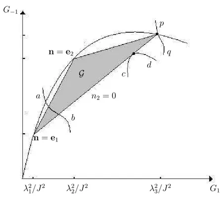
i (i= 1,2,3). Since the solution of the system (3.11) forn2
i has to be non–negative, the domain Gof admissible values for the orientation invariantsGl, G−1
is a triangle with vertexes lying on the parabolaJ2G2
1−I1G1+G−1 = 0
(Fig. 2).
The vertexes (λ−i 2λ−j2, λ−i 2+λ−j2) (i6=j) correspond to to n=ek (k6=i, j), t1 =t−1 = 0. On the i−j – side of the triangle
G−1 =G1λ2k+λk−2, nk = 0 (k6=i, j) (3.12) corresponding normalsnlie in thei−j−principal plane ofB,t1 kt−1.
The triangle G degenerates into the segment if λ1 = λ2 6= λ3 or
the point if λ1 = λ2 =λ3. Relations with the normals in the case are
evident.
Due to the kinematical condition (2.1), the invariants G1 and G−1
are continuous on the interface:
[[G1]] = 0, [[G−1]] = 0 (3.13)
The conditions (3.13) have obvious geometrical meanings. If da and
dA denote surface elements in deformed and reference configurations then it is simple to check that G1 = (dA/da)2. Then (3.13)1 means
that [[da]] = 0 at given dA. Analogously, (3.13)2 means that tangent
3.2
Kinematic compatibility
From (3.1), (3.5) follows thatB+ =B−+J−−1(c⊗B−n+B−n⊗c) +G−1c⊗c, (3.14)
B−+1 =B−−1−J−1
+ (n⊗B−−1c+B−−1c⊗n)
+J−2
+ (c·B−−1c)n⊗n.
(3.15) From (3.1) also follows
c= [[J]]n+h, h,Pc. (3.16) Then (3.14) – (3.15) lead to the following relationships between the strain and orientation invariants on the interface andh:
[[I1]] = G1[[J2]] + 2h·t−1 +G1h·h, (3.17)
[[I2]] = G−1[[J2]]−2h·t−−1+h·B−1h. (3.18)
3.3
Traction continuity condition
Projecting the traction condition (3.2) onto the normalnand the plane tangent to the shock surface and taking into account (3.6) we obtain
[[µ0]] + [[µ1N1]] + [[µ−1N−1]] = 0, (3.19)
[[µ1Jt1]] + [[µ−1J−1t−1]] = 0 (3.20)
The condition (3.19) for the normal component of the traction can be rewritten as
−[[W3]] = 2 [[JW1]]G1+ 2 [[JW2]]G−1. (3.21)
The equation (3.20) for the tangent component of the traction takes the form of an equation forh:
A+h=−[[W1]]t−1 + [[W2]]t−−1, A+ ,G1W1+I+W2+PB−1 (3.22)
and leads to the
Representation theorem[4]. Assume that the material is isotropic and on the shock surface the kinematic (3.1) and traction (3.2) condi-tions are satisfied and
D+=G1 W1+
2
+G−1W1+W2++ W2+
2
6
holds. Then the amplitudecis an isotropic function of the strain tensor
B− and the normal n and can be decomposed as follows:
c= [[J]]n+h, h=αt−1 +βt−−1 (3.24)
where the coefficients α and β are uniquely given as functions of ori-entation and strain invariants by the system of linear equations
G1W1+ W2+
−G1W2+ G1W1++G−1W2+
!
α β
!
= −[[W1]] [[W2]]
!
, (3.25)
The representation (3.24) remains true for incompressible materials; one needs only to set J ≡1.
There are physical and mathematical reasons to believe that the deformations cannot be observed if the Legendre-Hadamard condition fails. The Baker-Ericksen inequalities
W1+λ2kW2 >0 (k = 1,2,3) (3.26)
are the necessary conditions for strong ellipticity of isotropic nonlinear elastic materials. If (3.26) holds on the interface then (3.23) is satisfied at any G1, G−1 ∈ G and the amplitude is represented by (3.24), (3.25)
[7, 8, 9].
3.4
Thermodynamic condition. Phase transition
zone
The thermodynamic condition (3.3) takes the form
[[W]] =τn[[J]] + 2W1−h·t−1 −2W2−h·t−−1 (3.27)
where the normal component of the traction
τn =n·Tn= 2J(G1W1+G−1W2) +W3 (3.28)
can be calculated at any side of the phase boundary.
solution compatible with kinematic, traction and thermodynamic con-ditions, if it exists at givenI1−, I2−, J−, has a form of an one-parameter
family.
If we solve three of the equations for I1+ =I1+(G1, G−1|I1−, I2−, J−),
I2+ = I2+(G1, G−1|I1−, I2−, J−), J+ = J+(G1, G−1|I1−, I2−, J−), then the
forth equation takes the form of an equation for the one-parameter family of the orientation invariants:
Ψ(G1, G−1|I1−, I2−, J−) = 0. (3.29)
Since G1, G−1 ∈ G−, the invariants J−, I1− and I2− have to satisfy
inequalities min G1,G−1∈G−
Ψ(G1, G−1, J−, I1−)≤0≤ max
G1,G−1∈G−
Ψ(G1, G−1, J−, I1−).
(3.30) The one-parameter family of normals is represented on theG1, G−1–
plane by the intersection of the line (3.29) (the line abon Fig. 2) with the triangleG. The phase transition zone in λ1, λ2, λ3–space is formed
by all principal stretches at which the intersection is non-empty. If (λ1−, λ2−, λ3−) belongs to the PTZ boundary then the line of the
solu-tion passes through a single point ofG−, i.e. passes through the vertex
or externally touches the side of the triangle (the lines pq and cd on Fig. 2). In these cases the normal coincides with an eigenvector of B− or lies in a principal plane of B−; the one-parameter character of the
solution disappears.
To illustrate the PTZ in a case of finite strains construction we consider below two examples.
3.4.1 Phase transition zones for the Hadamard material
The strain energy function for the Hadamard material has the form
W = c
2I1+
d
2I2+ Φ(J), c≥0, d≥0, c+d6= 0. (3.31) General analysis of the PTZ construction for the Hadamard material was carried out in [4]. Below we give some illustrations.
Since [[W1]] = [[W2]] = 0, the representation theorem (see (3.25))
gives
G1
G−1
G
λ2
1/J2 λ22/J2 λ23/J2
n=e1
n=e2
n2 = 0
a
b
c d
q p
Figure 2: Admissible values domain G for the orientation invariants and lines of solutions.
The condition (3.21) for the normal component of traction and the thermodynamic condition (3.27) take the form
cG1+dG−1 =U(J+, J−), U(J+, J−),−
[[Φ′]]
[[J]], (3.33) [[W]] = (J−(cG1 +dG−1) + Φ′) [[J]] (Φ′ =
dΦ
dJ) (3.34)
Substituting (3.32) into kinematic relationships (3.17), (3.18) gives [[I1]] = [[J2]]G1, [[I2]] = [[J2]]G−1 (3.35)
Since
[[W]] = c 2[[I1]] +
d
from (3.33) – (3.35) follows 1
2(Φ
′
++ Φ′−)(J+−J−)−(Φ+−Φ−) = 0 (3.36)
The equation (3.36) can be solved forJ+ =J+(J−). Then (3.33) takes
the form of the equation that determines the one-parameter family of normals
cG1+dG−1 =u(J), u(J) =U(J+(J), J), G1, G−1 ∈ G− (3.37)
The left part of the equation (3.37) is linear in G1, G−1 and reaches
the minimal and maximal values in vertexes of the triangle G. If λ1 <
λ2 < λ3 then
min G1,G
−1⊂G
(cG1+dG−1) =h(λ2, λ3), n=e1
max G1,G
−1⊂G
(cG1+dG−1) =h(λ2, λ1), n=e3
h(λi, λj) =
c λiλj
+d
1
λi + 1
λj
Thus, the strains inside the PTZ satisfy the inequalities
h(λ2, λ3)≤u(J)≤h(λ2, λ1). (3.38)
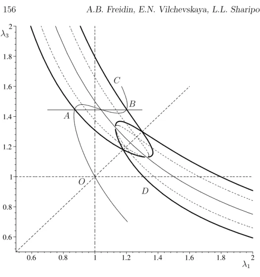
The typical PTZ cross-section by the plane λ2 =const is shown on
the Fig. 3. For the simplicity sake we take Φ(J) in a form
Φ(J) = (J−Jc)
4
4 −
A(J −Jc)2
2 +a(J−Jc). (3.39) Note that W 9 ∞ at J → 0 but one can consider (3.39) as an ap-proximation of Φ in the vicinity ofJc. SinceJ+ > Jc ifJ− < Jc on the interface [4], we take Jc > 1 and do not consider the behavior of the material at small J.
0.6 0.8 1 1.2 1.4 1.6 1.8
0.6 0.8 1 1.2 1.4 1.6 1.8 2
λ1
λ3
A
B C
D O
Figure 3: PTZ for the Hadamard material (Jc = 1.45, A = 0.3, d = 0.155, c= 0.03).
A and B. Only λ1 jumps on the interface. If the point D is reached,
the normal is directed as e3, λ3 jumps on the interface.
The line OAC represents the path of plane stretching in the “3”– direction in a case of uniform deformation - without the separation into two phases. In this case
λ2 = 1, λ1 = Λ(λ3)λ3, τ1(λ1, λ3) = 0 (3.40)
whereτ1 is the principal Cauchy stress and the function Λ(λ3) is found
from the condition (3.40)3.
sub-zone the sample can be divided into two phases before the non-ellipticity zone is reached. If A corresponds to the deformation on one side of the interface, then n =e1 and B corresponds to the
deforma-tions on the other side. Since τ1 remains to be zero after the plane
interface (interfaces) appear, the condition (3.40)3 does not fail
be-cause of internal stresses. Thus, the point B must belong to the curve
OAC. The role of internal stresses produced by phase transformations is demonstrated in the example given below.
3.4.2 Phase transition zones construction for compressible materials with strain energy depending on two strain invariants
Let W = W(Iα, J) (α = 1 or 2). Then, by (3.24), (3.25), (3.17) and (3.18)
h=− [[Wα]]
W+
αG1
t−1, (3.41)
[[I1]] =G1[[J2]]−
[[W2
α]]
W2
α+
L−1, [[I2]] = G−1[[J2]]−
[[W2
α]]
W2
α+
L−2, (3.42)
L1 =I1−J2G1−G−1G−11, L2 =I2 −J2G−1−G−11, (3.43)
If W = W(I1, J) then the conditions (3.21) and (3.27) take the
form
2G1[[JW1]] =−[[W3]], (3.44)
[[W]] = W
−
1 W3++W1+W3−
W1−+W1+ [[J]] +
2W1−W1+
W1−+W1+[[I1]]. (3.45)
Relationships (3.42)1, (3.44) and (3.45) are three equations for the
four unknowns J+, I1+, G1 and G−1. If we solve (3.44) and (3.45) to
obtain
J+ =J+(G1, J−, I1−), I1+ =I1+(G1−, J−, I1−), (3.46)
and substitute the expressions into (3.42), we derive an equation in the form
The equation (3.47) determines a line of one-parameter solutions on the G1, G−1–plane.
The invariants J− and I1− have to satisfy inequalities
Ψmin(J−, I1−)≤0≤Ψmax(J−, I1−),
Ψmin(J−, I1−) = G min
1,G −1∈G−
Ψ(G1, G−1, J−, I1−),
Ψmax(J−, I1−) = G max
1,G −1∈G−
Ψ(G1, G−1, J−, I1−).
Since Ψ(G1, G−1, J−, I1−) is linear in G−1, its maximal and minimal
values are reached at the boundary of G−. The corresponding normal
lies in the principal planes of B− or coincide with the eigenvector of B−. Thus, three types of strain localization due to phase transitions
can be expected if the interface corresponds to the PTZ boundary: (1) the interface is analogous to the shear band, plane jump of strains takes place on the interface, (2)the interface is perpendicular to the direction of the maximal stretch, only the maximal stretch suffers a jump on the phase boundary, (3) the interface is perpendicular to the direction of the minimal stretch that suffers a jump.
Materials with a potential W =W(I2, J) may be considered
anal-ogously. Let
W(I1, J) = V(I1) + Φ(J) (3.48)
where
V(I1) =
c1I1, I1 ∈(0, Ic)
c2(I1−Ic) +c1Ic, I1 ∈(Ic,∞) , c1 > c2, (3.49) Φ(J) =aJ2+bJ +c
where the coefficient a > 0 characterize the reaction of the material with respect to volume changing. A “kink” in a point I1 =Ic replaces the non-ellipticity sub-zone.
The conditions on the equilibrium interface (3.42)1, (3.44) and
(3.45) take the form
[I1] = (γ2 −1)G1J−2 + (k2−1)L−1 (3.50)
λ1
λ3
O A B C D
P T
Q S
1 1
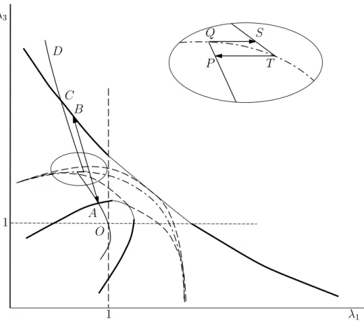
Figure 4: PTZ for the model material in a plane case.
[I1] = (k+ 1)(Ic−I1−)−AJ−2(γ−1)2 (3.52)
whereγ =J+/J−,k=c1/c2,A =a/c2andL1 is determined by (3.43)1.
The equation (3.51) can be solved forγ =γ(G1). Then substituting
(3.50) into (3.52) leads to the following relationship for the orientation invariants
J2
−G21
A+G1
+L−1 = Ic−I
−
1
k−1 (3.53)
The “−”– PTZ subzone is determined by the inequalities
min G1,G−1∈G
J2
−G21
A+G1
+L−1 ≤ Ic−I
−
1
k−1 ≤G1max,G−1∈G J2
−G21
A+G1
+L−1 (3.54)
The PTZ cross-section for the material (3.48) is shown at Fig. 4 at A > k. The dot-and-dash line corresponds to I1 = Ic. Thick lines correspond to “shear bands”. In this case the normal to the interface lies in a plane of maximal and minimal stretches. A shear parameter contributes to the jump of strains.
If thin lines are reached then the interfaces may appear which are perpendicular to the direction of the maximal principal stretch, and only this stretch suffers a jump.
Dotted lines denote internal PTZ boundaries. Corresponding inter-faces are perpendicular to the direction of minimal stretching. Thus, depending on the deformation path various types of strain localization are possible due to phase transformations.
The competition between the types of the interfaces also depends on the material parameters. If A ≫k then interfaces of shear band type are preferential if the PTZ boundary is reached. The angle between the interface and the direction of the maximal stretch is about π/4. If the parameter A decreases then the angle increases, and interfaces perpendicular to the direction of maximal stretching can also appear.
At A≈k the difference between two types of the interfaces disap-pears. IfA < A∗ then only the interfaces perpendicular to the maximal
stretching correspond to the PTZ boundary, where A∗ depends on k
and Ic.
The lineOACD represents plane stretching in the “3”– direction in a case of uniform deformation - without the separation into two phases. Note that in the vicinity of the line I = Ic the behavior at loading and unloading includes hysteresis P QST. Similar to the Hadamard material, two-phase deformation can appear before the line I = Ic is reached.
Since the PTZ construction arises from the analysis of the local equilibrium conditions, every point of the PTZ corresponds to some piece-wise linear two-phase deformation with plane interfaces. Points
A and B represent such a deformation. If the point A is reached on the path OAQ, one can suppose that a thin layer of the phase “+” appears in an unbounded media and the point B corresponds to the deformation inside the layer.
belong to the curveDCS, in contrast to the Hadamard material. Anal-ogously, if the point C is reached on the pathDCS, appearance of the layer of the phase “−” surrounded by the phase “+” can be assumed. In conclusion note that we do not study here how the phase “−” transforms into the phase “+”. In a case of heterogeneous deformation due to multiple appearance of a new phase areas average deformations are prescribed by boundary conditions. Two-phase structures have to be found but the local deformations on the interfaces belong to the PTZ.
4
Equilibrium phase boundaries
in a case of small strains
In a case of small strains a problem on equilibrium two-phase config-urations of elastic bodies can be reduced to the determination of the phase boundary Γ and displacementsu(x) smooth enough at material points x∈/Γ, continuous on Γ
[[u]] = 0, x∈Γ (4.1)
and satisfying boundary conditions, thermal condition θ = const, and equilibrium conditions
x∈/ Γ : Divσ = 0, (4.2)
x∈Γ : [[σ]]n= 0, [[f]]−σ: [[ε]] = 0 (4.3) where σ and ε are the stress and strain tensors, θ is the temperature,
f(ε, θ) is the volume free energy density represented by a number of quadratic function of ε.
Further, for the sake of simplicity, we consider two-branches free energy function
f(ε, θ) = min
−,+
f−(ε, θ), f+(ε, θ) , (4.4)
f±(ε, θ) = f±
0 (θ) +
1 2(ε−ε
p
±) :C±: (ε−εp±) The constitutive equations take the form:
σ(ε) =C±: (ε−εp
ParametersC±, f0±, ε
p
± are the elasticity tensors, free energy densities
and strain tensors in unstressed phases “±”. If εp+ = 0, then [εp]≡εp is the self–strain tensor. Body forces and thermoelastic effects are not taken into account. Twinning also is not studied here.
It follows from (4.1), (4.3)1, (4.5), that [16, 6]
[ε] =K∓(n) :q±, q± =−C1:ε±+ [C:εp], (4.6) K±(n) ={n⊗G±⊗n}s, G± = (n·C±·n)−1, C1 =C+−C−,
s means the symmetrization: Kijkl = n(iGj)(knl). Substituting (4.4),
(4.5) and (4.6) into (4.3)2 brings the thermodynamic condition to the
form [15, 6]
2γ+[εp:C:ε p]+ε±:C1:ε±−2ε±: [C:εp]±q±:K∓(n) :q± = 0 (4.7) where γ = [f0(θ)] acts as temperature in absence of thermal stresses.
So, the system of equations is split. Given γ, any of two equations (4.5) determines one-parametric family of unit normals depending on strains on one side (“+” or “−”) of the interface. Strains on the other side can be computed by formulas (4.6).
If tensor C1 is nonsingular, the equations (4.7) can be rewritten in
q – space:
K∓(q±,n) =∓ϕ(q±), (4.8)
K±(q,n) = q:K±(n) :q, ϕ(q) = 2γ∗+q:C−11:q,
γ∗ =γ+
1 2[ε
p] :B−1
1 : [εp], C1 =C+−C−, B1 =B+−B−, B=C−1.
Strains for which the equation (4.7) or (4.8) can be solved for the unit normal n form the phase transition zone in ε– or q–space. Note that the equation ϕ(q = 0) determines the surface of discontinuity in the derivative off(ε) where f+(ε=f−(ε).
The PTZ is divided into sub–zones Q±. By (4.8), tensors q± ∈ Q±
satisfy inequalities
Kmin∓ (q±)≤ ∓ϕ(q±)≤ K∓max(q±), (4.9)
K∓max(q±) = max
n K∓(q,n), K
∓
min(q±) = min
The normals n±ex(q) andn±in(q) afford a maximum and a minimum to
K∓(q±,n), respectively, and correspond to the external and internal
boundaries of the sub–zones Q± [17, 6]. Note that the tensor q+ can
be related with the tensor of the dislocation moments induce by new phase areas [16].
If phase “−” is isotropic, maximal and minimal values ofK−(q+,n)
as well as corresponding normals depend on relations between the eigenvalues qi of q+ [3, 17, 6]. Let q1 ≤ q2 ≤q3, q1 6=q3, |q|min, |q|max
are the minimal and maximal absolute values of the eigenvalues, e|q|min
e|q|max are the corresponding eigenvectors, ni are the components of the normal n in the basis of eigenvectors of q+.
If q1q3 <0 or q1q3 >0, (1−ν−)|q|min < ν−|q|max, then
n23 = (1−ν−)q3−ν−q1
q3−q1
, n2 = 0,
µ−K−max(q+) =
1−ν−
2 (q
2
1 +q32)−ν−q1q3.
The plane jump of strains similar to shearing takes place on the inter-face.
In the other case
nex(q+) =e|q|max, K−max(q+) =
1−2ν−
2µ−(1−ν−)
|q|2max. (4.10)
Only maximal eigenvalue of the strain tensor suffers a jump on the interface.
At minimal value of K−(q+,n)
nin(q+) =e|q|min, Kmax− (q+) =
1−2ν−
2µ−(1−ν−)
|q|2min. (4.11)
Only minimal eigenvalue of the strain tensor suffers a jump.
Thus, if q+ on the interface belongs to the external PTZ boundary
then, depending on a relation between eigenvalues of q+, the normal n lies in the 1−3 – principal plane of the tensor q+ or coincides with
the eigenvector e|q|max. On the internal PTZ boundary (4.11) holds.
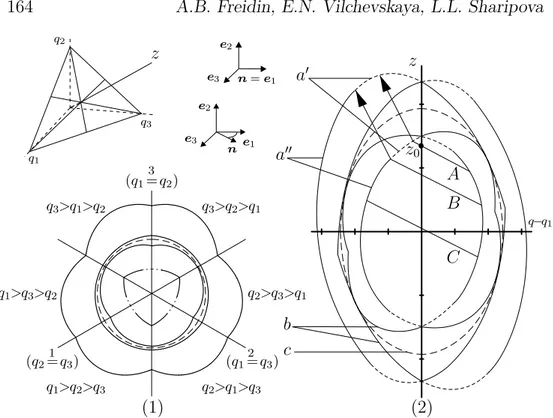
(1) (2) q1
q3 z
e3 n=e1
e3 e2
e1 n
a′
a′′
b c
A B
C z0
z
q−q1
3
(q1=q2)
2
(q1=q3)
1
(q2=q3)
q3>q2>q1
q2>q3>q1
q2>q1>q3
q1>q2>q3
q1>q3>q2
q3>q1>q2
Figure 5: PTZ cross-sections: (1) - by the plane trq = const, (2) - by the plane q2 = q3 = q; a′ and a” - external PTZ boundaries;
b - internal PTZ boundaries; c - the surface of discontinuity in the derivative off(ε); z0 corresponds to the undeformed state.
Acknowledgements
The help of the student M. Stepanenko is gratefully acknowledged. This work is supported by the Russian Foundation for Basic Research (Grants No. 01-01-00324, 02-01-06263) and the Program of Ministry of Industry and Sciences of Russian Federation (Project No. 40.010.1 1.1195).
References
[1] R. Abeyaratne and J.K. Knowles,Equilibrium shocks in plane deforma-tion of incompressible elastic materials. J. Elasticity 22(1989) 63–92.
[2] R.L. Fosdick and B. Hertog, The Maxwell relation and Eshelby’s con-servation law for minimizers in elasticity theory.J. Elasticity22(1989)
193–200.
[3] A.B. Freidin, Crazes and shear bands in glassy polymer as layers of a new phase. Mekhanika Kompozitnih Materialov, No. 1, 3-10 (1989). (Mechanics of Composite Materials, 1-7 (1989)).
[4] A.B. Freidin and A.M. Chiskis, Phase transition zones in nonlin-ear elastic isotropic materials. Part 1: Basic relations. Izv. RAN, Mekhanika Tverdogo Tela (Mechanics of Solids) 29 (1994) No. 4, 91–
109.
[5] A.B. Freidin and A.M. Chiskis, Phase transition zones in nonlin-ear elastic isotropic materials. Part 2: Incompressible materials with a potential depending on one of deformation invariants. Izv. RAN, Mekhanika Tverdogo Tela (Mechanics of Solids)29 (1994) No. 5, 46–
58.
[6] A.B. Freidin,Small strains approach to the theory on solid-solid phase transformations under the process of deformation.Studies on Elasticity and Plasticity (St. Petersburg State University)18(1999) 266-290 (in
Russian).
[8] A.B. Freidin, On phase equilibrium in nonlinear elastic materials.
Nonlinear problems of continuum mechanics. Izvestia Vuzov. North-Caucasus region (2000) 150-168 (in Russian)
[9] A.B. Freidin, Two-phase deformation fields and ellipticity of nonlin-ear elastic materials.Proceed. of the XXVIII Summer School “Actual Problems in Mechanics”, St.Petersburg, Russia, June 1-10, 2000. Vol. 1, 219-235 (2001)
[10] M.A. Grinfeld, On conditions of thermodynamic equilibrium of the phases of a nonlinear elastic material. Dokl. Acad. Nauk SSSR 251
(1980) 824–827.
[11] M.E. Gurtin, Two–phase deformations of elastic solids. Arch. Rat. Mech. Anal.84(1983) 1–29.
[12] R.D. James, Finite deformation by mechanical twinning. Arch. Rat. Mech. Anal.77(1981) 143–177.
[13] J.K. Knowles and E. Sternberg, On the failure of ellipticity and the emergence of discontinuous deformation gradients in plane finite elas-tostatics.J. Elasticity 8 (1978) 329–379.
[14] J.K. Knowles,On the dissipation associated with equilibrium shocks in finite elasticity. J. Elasticity 9 (1979) 131–158.
[15] L.B. Kublanov and A.B. Freidin, Solid phase seeds in a deformable material. Prikladnaia Matematica i Mekhanika, 52 (1988), 493-501. (
Journal of Applied Mathematics and Mechanics (PMM U.S.S.R.), 52
(1988), 382-389).
[16] I.A.Kunin. Elastic Media with Microstructure II. Springer-Verlag, Berlin, New York, etc. (1983).
[17] N.F. Morozov and A.B. Freidin, Phase transition zones and phase transformations of elastic solids under different stress states. Proceed-ings of the Steklov Mathematical Institute223 (1998) 220–232.
[19] L. Truskinovsky,Equilibrium interphase boundaries.Dokl. Acad. Nauk SSSR 265 (1982) 306–310.
[20] G. Truesdell, A First Course in Rational Continuum Mechanics. The Johns Hopkins Univercity, Baltimore, Maryland (1972).
Dvofazne deformacije unutar zona faznih prenosa
UDK 531.01, 532.59, 536.76