TESE SE DOUTORADO No 126
THE DETECTION OF SPATIAL CLUSTERS: GRAPH AND DYNAMIC PROGRAMMING METHODS
Gladston Juliano Prates Moreira
Universidade Federal de Minas Gerais
Programa de P´os-Graduac¸˜ao em Engenharia El´etricaThe Detection of Spatial Clusters:
Graph and
Dynamic Programming Based Methods
Gladston Juliano Prates Moreira
Thesis presented to the Graduate Program in Electrical Engineer of the Federal University of Minas Gerais in final fulfillment of the require-ments for the degree of Doctor in Electrical En-gineer.
Advisor: Prof. Luiz Henrique Duczmal Co-advisor: Prof. Ricardo H. C. Takahashi
During the development of this work the author received financial support from CAPES / FAPEMIG
Universidade Federal de Minas Gerais
Programa de P´os-Graduac¸˜ao em Engenharia El´etricaA Detec¸
c~
ao de
Clusters
Espaciais:
M´
etodos Baseados
em Grafos e Programa¸
c~
ao Din^
amica.
Gladston Juliano Prates Moreira
Tese submetida ao Programa de P´os-Gradua¸c˜ao em Engenharia El´etrica da Universidade Fede-ral de Minas Gerais, como requisito final para obten¸c˜ao do t´ıtulo de Doutor em Engenharia El´etrica.
Orientador: Prof. Luiz Henrique Duczmal Co-orientador: Prof. Ricardo H. C. Takahashi
Durante o desenvolvimento deste trabalho o autor recebeu aux´ılio financeiro da CAPES/FAPEMIG
Dedico esse trabalho `a Raquel, Rossana e ao meu filho Gael.
I dedicate this work to Raquel, Rossana and my son Gael.
Acknowledgments
I would like to thank first my whole family, specially my parents for their support, comprehension and for everything they have done for me.
I am also very grateful to Jussara, David, Eloy, Anderson and Emerson for the great friendship and companionship.
Thanks to Professor Luiz Henrique Duczmal and Professor Ricardo Taka-hashi which were essential in this work. Thanks for the shared knowledge, the excellent orientation, the credit and the opportunity given to me.
I am grateful to Fl´avia Magalh˜aes, the community of health agents of the Family Health Program, and the Secretary of Health and Epidemiological Surveillance in Lassance City.
Thanks also to Professor Lu´ıs Paquete the great opportunity that he offered me, the excellent orientation and assistance during the Phd internship I worked at the University of Coimbra. I also thank Professor Carlos Fonseca by the doors that were opened.
Many thanks to the members of my thesis committee, professors Lu´ıs Pa-quete, Rodney Rezende Saldanha, Andr´e Luiz Fernandes Can¸cado, Elizabeth Fialho Wanner and Denise Burgarelli Duczmal for their valuable suggestions. I am grateful to colleagues in the group’s statistics department and engi-neering school for help and companionship.
I would like to thank CAPES and FAPEMIG for the financial support and everyone that contributed to this work.
Agradecimentos
Gostaria de agradecer primeiramente toda minha fam´ılia, especialmente ao meus pais, pelo apoio e por tudo que fizeram por mim.
Sou muito grato tamb´em `a Jussara, David, Eloy, Anderson e Emerson pela grande amizade e companherismo.
Agrade¸co ao Professor Luiz Henrique Duczmal e Professor Ricardo Taka-hashi os quais foram essenciais na realiza¸c˜ao deste trabalho. Agrade¸co pelo conhecimento compartilhado, pela excelente orienta¸c˜ao, pela confian¸ca e pela oportundade que me foi dada.
Agrade¸co a Fl´avia Magalh˜aes, a comunidade dos agentes de sa´ude do Pro-grama Sa´ude da Fam´ılia e a secretaria de Sa´ude e Vigilˆancia Epidemiol´ogica da cidade de Lassance.
Agrade¸co tamb´em ao Professor Lu´ıs Paquete, pela grande oportunidade que ele me proporcionou, pela excelente orienta¸c˜ao e acolhimento durante o doutorado sandu´ıche realizado na Universidade de Coimbra. Agrade¸co tamb´em ao Professor Carlos Fonseca pelas portas que foram abertas.
Gostaria tamb´eem de agradecer aos membros da minha banca, os pro-fessores Lu´ıs Paquete, Rodney Rezende Saldanha, Andr´e Luiz Fernandes Can¸cado, Elizabeth Fialho Wanner e Denise Burgarelli Duczmal pelas valiosas sugest˜oes
Sou grato aos colegas do grupo do departamento da estat´ıstica e da escola de engenharia pelo grande companheirismo.
Meus agradecimentos `a CAPES e FAPEMIG pelo suporte financeiro e a todos aqueles que de alguma forma contribu´ıram para a realiza¸c˜aao deste trabalho.
Abstract
This thesis addresses the spatial and space-time cluster detection prob-lem. Two algorithms to solve the typical problem for spatial data sets are proposed.
A fast method for the detection and inference of point data set spatial and space-time disease clusters is presented, the Voronoi Based Scan (VBScan). A Voronoi diagram is built for points representing population individuals (cases and controls). The number of Voronoi cells boundaries intercepted by the line segment joining two cases points defines the Voronoi distance between those points. This distance is used to approximate the density of the heterogeneous population and build the Voronoi distance Minimum Spanning Tree (VMST) linking the cases. The successive removal of edges from the VMST generates sub-trees which are the potential clusters. Finally, those clusters are evaluated through the scan statistic. Monte Carlo replications of the original data are used to evaluate the significance of the clusters. The ability to promptly detect space-time clusters of disease outbreaks, when the number of individuals is large, was shown to be feasible, due to the reduced computational load of VBScan. Numerical simulations showed that VBScan has higher power of detection, sensitivity and positive predicted value than the Elliptic PST. Furthermore, an application for dengue fever in a small Brazilian city is presented.
In a second approach, the typical spatial cluster detection problem is reformulated as a bi-objective combinatorial optimization problem. We pro-pose an exact algorithm based on dynamic programming, Geographical Dy-namic Scan, which empirically was able to solve instances up to large size within a reasonable computational time. We show that the set of
vi
dominated solutions of the problem, computed efficiently, contains the so-lution that maximizes the Kulldorff’s Spatial Scan Statistic. The method allows arbitrary shaped clusters, which can be a collection of disconnected or connected areas, taking into account a geometric constraint. Note that this is not a serious disadvantage, provided that there is not a huge gap between its component areas. We present an empirical comparison of detection and spatial accuracy between our algorithm and the classical Kulldorff’s Circular Scan, using the data set of Chagas disease cases in puerperal women in Minas Gerais state, Brazil.
Resumo
Esta tese aborda o problema de detec¸c˜ao de clusters espaciais e espa¸cos-temporais. Dois algoritmos para resolver o t´ıpico problema de conjuntos de dados com processos espaciais s˜ao propostos.
Um m´etodo eficiente para a detec¸c˜ao e inferˆencia de clusters de doen¸cas espaciais e espa¸cos-temporais de dados pontuais ´e apresentado, o Voronoi Based Scan (VBScan). Um diagrama de Voronoi ´e constru´ıdo para os pontos que representam indiv´ıduos da popula¸c˜ao (casos e controles). O n´umero de c´elulas de Voronoi interceptadas pelo segmento de linha que une de dois pontos que representam dois casos define a distˆancia de Voronoi entre esses pontos. Esta distˆancia ´e usada para aproximar a densidade da popula¸c˜ao heterogˆenea e construir a ´arvore geradora m´ınima baseada na distˆancia de Voronoi (VMST) ligando os casos. A remo¸c˜ao sucessiva de arestas da VMST gera sub-´arvores que s˜ao os clusters candidatos potenciais. Finalmente, os clusters s˜ao avaliados atrav´es da estat´ıstica scan de Kulldorff. Simula¸c˜oes de Monte Carlo dos dados originais s˜ao usados para avaliar a significˆancia dos clusters. A capacidade de detectar rapidamente clusters de surtos da doen¸ca, quando o n´umero de indiv´ıduos ´e grande, mostrou-se vi´avel, devido `a redu¸c˜ao da carga computacional obtida com o VBScan. As simula¸c˜oes num´ericas mostraram que o VBScan tem maior poder de detec¸c˜ao, sensibilidade e valor preditivo positivo do que o scan el´ıptico. Al´em disso, uma aplica¸c˜ao de casos e controles georeferenciados de dengue em uma cidade do Brasil ´e apresentado. Numa segunda abordagem, o problema t´ıpico de detec¸c˜ao de clusters espaciais ´e reformulado como um problema bi-objetivo de otimiza¸c˜ao com-binat´oria. N´os propomos um algoritmo exato baseado em programa¸c˜ao dinˆamica, Geographical Dynamic Scan, que empiricamente foi capaz de
viii
solver os casos at´e de grande porte dentro de tempo computacional aceit´avel. N´os mostramos que o conjunto de solu¸c˜oes n˜ao dominadas do problema, en-contradas eficientemente, cont´em a solu¸c˜ao que maximiza a estat´ıstica scan de Kulldorf. O m´etodo permite clusters de formatos arbitr´arios, que podem ser uma cole¸c˜ao de regi˜oes desconectadas ou conectadas, tendo em conta uma restri¸c˜ao geogr´afica. Note-se que esta n˜ao ´e uma s´eria desvantagem, desde que n˜ao haja um grande espa¸camento entre as suas ´areas. Apresentamos uma compara¸c˜ao emp´ırica de detec¸c˜ao e precis˜ao espacial entre o nosso algoritmo e o cl´assico Scan circular, utilizando dados de casos de doen¸ca de Chagas em mulheres parturientes no estado de Minas Gerais, Brasil.
Resumo Estendido
Esta se¸c˜ao consiste em um resumo estendido sobre o trabalho desenvolvido nesta tese. Primeiramente, este texto introduz o problema abordado, a prin-cipal motiva¸c˜ao para solucion´a-lo e alguns dos principais m´etodos relaciona-dos. Em seguida, uma breve descri¸c˜ao dos objetivos principais das metodolo-gias desenvolvidas para resolver o problema. Finalmente, as conclus˜oes s˜ao apresentadas.
Introdu¸c˜
ao
Testes estat´ısticos de vigilˆancia de doen¸ca no espa¸co e no espa¸co-tempo, geralmente, procuram determinar se a incidˆencia da doen¸ca em um sub-conjunto definido espacial e/ou temporalmente ´e incomum em rela¸c˜ao `a in-cidˆencia na regi˜ao de estudo como um todo. Assim, essa classe de m´etodos ´e projetada para detectar clusters de doen¸ca no espa¸co e no tempo, e adaptar sistemas de vigilˆancia concebidos para a detec¸c˜ao de surtos. O desenvolvi-mento de m´etodos de detec¸c˜ao de clusters espa¸cos-temporais, naturalmente, evoluiu a partir de m´etodos puramente espaciais. Podemos estratificar os m´etodos em trˆes tipos de classe de testes estat´ısticos: testes para intera¸c˜ao espa¸co-tempo, os m´etodos de soma cumulativa, e a estat´ıstica scan.
A estat´ıstica espacial scan de Kulldorff (Kulldorff, 1997) ´e atualmente o m´etodo mais usual para encontrar clusters (aglomerados) espaciais, espa¸co-temporais e espa¸co-temporais. Estudada em detalhe pela primeira vez por (Naus,
1965) ´e um m´etodo estat´ıstico com muitas aplica¸c˜oes potenciais, com o ob-jetivo de detectar um excesso de eventos locais. A estat´ıstica espacial scan supera o problema de testes m´ultiplos (comuns a muitos m´etodos locais de
x
an´alise espacial), tomando o cluster mais prov´avel definido pela maximiza¸c˜ao da raz˜ao de verossimilhan¸ca. (Kulldorff & Nagarwalla, 1995) apresentam o cl´assico Scan Circular, um teste que encontra o cluster mais veross´ımil dentre todas as zonas circunscritas por c´ırculos de raios variados centrados em cada regi˜ao do mapa.
Em (Kulldorff,2001), a estat´ıstica espacial scan ´e estendida para o
espa¸co-tempo, de modo que cilindros s˜ao utilizadas para o formato dos potenciais candidatos a cluster. A base circular representa a ´area espacial e a altura do cilindro representa o per´ıodo de tempo. Na an´alise prospectiva, cilindros candidatos s˜ao limitados `aqueles que come¸cam a qualquer momento durante o per´ıodo de estudo e termina no per´ıodo de tempo atual (ou seja, clusters vivos).
O problema t´ıpico de detec¸c˜
ao de clusters
es-paciais
No enfoque desta tese, propomos dois m´etodos de detec¸c˜ao de clusters espaciais quando dois tipos de dados de processo espacial para um determi-nado fenˆomeno de interesse est˜ao dispon´ıveis. Suponha que tenhamos, por exemplo, um mapa dividido em regi˜oes, cada uma delas com uma popula¸c˜ao conhecida e um n´umero de casos observados. Assim, cada caso pode ser, por exemplo, um indiv´ıduo infectado por uma certa doen¸ca. Neste mapa um
cluster ´e um aglomerado de regi˜oes geograficamente limitadas onde o risco de ocorrˆencia do fenˆomeno de interesse ´e muito elevado ou muito baixo com-parado com o risco das demais regi˜oes, e ao mesmo tempo significativo do ponto de vista estat´ıstico.
xi
Figure 1: Uma poss´ıvel zona obtida para uma dada janela circular.
de casos e controles, onde cada ponto no mapa representa indiv´ıduos infec-tados (casos) e indiv´ıduos com similares caracter´ısticas mas n˜ao infecinfec-tados (controles). Uma zona ´e qualquer subconjunto geograficamente limitado de indiv´ıduos do mapa. Dentre os N indiv´ıduos, n s˜ao casos e N −n s˜ao con-troles. Para cada c´ırculo de raio r > 0 centrado em cada indiv´ıduo, uma zona ´e o conjunto de indiv´ıduos dentro do c´ırculo. Um exemplo ´e visto na Figura 2.
Seja z ∈Z uma zona, definindo L(z) como a fun¸c˜ao de verossimilhan¸ca sob a hip´otese alternativa de que exista uma zona z∗
que ´e um cluster, e L0 como a verossimilhan¸ca sob a hip´otese nula de que n˜ao exista um cluster, foi mostrado em (Kulldorff,1997) que o logaritmo da raz˜ao de verossimilhan¸ca, K(z) = log (L(z)/L0), ´e dado por
K(z) =
Clog N C
+zClog
zC
zN
+ (C−zC) log
C
−zC
N −zN
if zC
zN
> C−zC N −zN
0 otherwise
(1) assumindo que o n´umero de casos na zona z, zC, segue uma distribui¸c˜ao
de Poisson com m´edia proporcional `a sua popula¸c˜ao zN. A fun¸c˜ao K ´e
xii
Figure 2: Uma poss´ıvel zona obtida para uma dada janela circular.
o cluster mais veross´ımil. Ent˜ao, temos a estat´ıstica de teste dada por T = maxzK(z).
A busca por solu¸c˜oes eficientes seria feita ent˜ao dentro do conjuntoZ. O fato ´e que seria computacionalmente inv´ıavel testar todas as zonas poss´ıveis. Para contornar esse problema, os algoritmos para detec¸c˜ao de clusters espa-ciais fazem uso de duas t´ecnicas:
• Redu¸c˜ao do conjunto das solu¸c˜oes canditadas Z para outro conjunto Z′
das zonas promissoras ou que permita uma busca exaustiva.
• Utiliza¸c˜ao de m´etodos estoc´asticos de otimiza¸c˜ao.
xiii
controlar as formas dos clusters encontrados. A solu¸c˜ao pode `as vezes se es-palhar atrav´es de diversas regi˜oes do mapa, fazendo com que se torne dif´ıcil a avalia¸c˜ao de seu significado geogr´afico. Outros apresentam clusters detec-tados com formatos fixos, tipicamente circulares.
Neste sentido, propomos nesta tese dois algoritmos distintos de detec¸c˜ao de clusters. Um que aborda conceitos de teoria de grafos, com o prop´osito de obter um conjuntoZ′
de potenciais candidatos a cluster. O outro implementa conceito de programa¸c˜ao dinˆamica com o objetivo final de reduzir o conjunto das solu¸c˜oes candidatas ao cluster, encontrando uma solu¸c˜ao ´otima global para o problema.
Conclus˜
oes
Este trabalho apresenta dois m´etodos de detec¸c˜ao de clusters espaci-ais. Um primeiro m´etodo direcionado a detectar clusters espaciais e espa¸co-temporais para dados de processos pontuais de casos e controles. O segundo direcionado a ambos os tipos de dados. Os m´etodos discutidos s˜ao eficientes na melhoria das medidas de avalia¸c˜ao utilizadas em compara¸c˜ao com m´etodos cl´assicos.
Principais contribui¸c˜
oes
• Proposi¸c˜ao de um algoritmo de detec¸c˜ao de cluster espaciais e espa¸co-temporais,Voronoi Based Scan, quando dispon´ıveis dados de processos pontuais de casos e controle;
• Proposi¸c˜ao de um algoritmo de cluster espaciais,Geographical Dynamic Scan, tanto para dados de ´area quanto para dados pontuais de casos e controle;
xiv
Esbo¸co da tese
Esta tese est´a organizada em 6 cap´ıtulos. O cap´ıtulo 1 apresenta os conceitos gerais do m´etodo de detec¸c˜ao de clusters espaciais, a estat´ıstica scan espacial, tipos de dados aplic´aveis, inferˆencia. Traz ainda uma breve descri¸c˜ao do m´etodo cl´assico para an´alise prospectiva de clusters espa¸co-temporais e uma breve revis˜ao da literatura.
O cap´ıtulo 2 apresenta nosso m´etodo proposto para detec¸c˜ao de clus-ters espaciais e espa¸co-temporais quando um conjunto de dados de processos pontuais do tipo caso-controle ´e avaliado. Ele utiliza conceitos de teoria de grafos e otimiza¸c˜ao geom´etrica para caracterizar as solu¸c˜oes candidatas a cluster. J´a no cap´ıtulo 3 implementamos um outro m´etodo de detec¸c˜ao de clusters espaciais usando um algoritmo de programa¸c˜ao dinˆamica que encon-tra eficientemente as solu¸c˜oes candidatas. Neste ´ultimo, tanto um conjunto de dados agregadoa ou pontuais podem ser avaliado.
No cap´ıtulo 4 apresentamos an´alises num´ericas que mostram o desem-penho dos m´etodos aqui propostos na detec¸c˜ao de clusters. Estudos com dados artificiais e dados reais encontrados na literatura foram realizados. No cap´ıtulo 5 uma aplica¸c˜ao de casos e controles georeferenciados de dengue na cidade de Lassance em Minas Gerais ´e apresentada.
Contents
List of Acronyms xvii
List of Figures xviii
List of Tables xxi
1 The spatial scan statistics 1
1.1 Types of Data . . . 1
1.1.1 Point Data . . . 1
1.1.2 Case-Control Data . . . 1
1.1.3 Aggregated Data . . . 2
1.1.4 Space Time Data . . . 3
1.2 Kulldorff’s Spatial Scan Statistic . . . 4
1.3 Spatial Cluster Inference . . . 5
1.4 Prospective Space-Time Scan . . . 6
1.5 State-of-the-art . . . 7
2 Voronoi based scans for point data sets 9 2.1 Motivation . . . 9
2.2 Definitions and Methods . . . 11
2.2.1 Minimum spanning tree representation . . . 12
2.3 Voronoi based spatial scan . . . 14
2.4 Voronoi based space-time scan . . . 17
3 Dynamic Programming based Scan 19 3.1 Motivation . . . 19
CONTENTS xvi
3.2 Multi-objective optimization problem . . . 20
3.3 System and Method . . . 22
3.3.1 Mathematical Formulation . . . 22
3.3.2 Dynamic programming algorithm . . . 24
3.4 Geographical dynamic scan . . . 27
4 Results and Discussion 30 4.1 Evaluated Measures . . . 30
4.2 Numerical Tests . . . 31
4.2.1 Voronoi Based Scan . . . 32
4.2.2 Geographical dynamic scan . . . 37
5 Application: A real dataset 50 5.1 Dengue Fever Clusters . . . 50
5.1.1 Spatial analysis . . . 52
5.1.2 Detecting space-time clusters . . . 55
6 Conclusions 58 6.1 Summary . . . 58
6.2 Publications . . . 60
6.3 Future Work . . . 61
List of Acronyms
VBScan - Voronoi Based Scan
VMST - Voronoi Minimum Spanning Tree
Elliptic PST - Elliptic Prospective Space Time
MST - Minimum Spanning Tree
GDScan - Geographical Dynamic Scan
ND - Non-dominated operator
PPV - Positive Predicted Value
FHP - Family Health Program
List of Figures
1 Uma poss´ıvel zona obtida para uma dada janela circular. . . . xi
2 Uma poss´ıvel zona obtida para uma dada janela circular. . . . xii
1.1 Spatial distribution of the observed cases in arbitrary data. . . 2
1.2 Spatial distribution of the observed cases (circles) and controls (dots) in Lancashire-UK data. . . 3
1.3 Mapping spatial variations of Chagas disease in the State of Minas Gerais - Brazil by county during 2006: (a) disease rates map; (b) Population at risk map. . . 4
2.1 An minimum spanning tree connecting all the data points, using Euclidean distance. . . 13
2.2 Left: spatial distribution of the 10 observed cases (circles) and 60 non-cases (dots). Right: corresponding Voronoi minimum spanning tree. . . 15
2.3 Visualization of the greedy edge deletion procedure, in suc-cessive steps numbered from 1 to 10. Sub-graphs linking blue circles represent the new cluster candidates that appear in each iteration, and sub-graphs linking black circles represent cluster candidates that have already appeared in former steps. 16
2.4 The “region of influence” of each individual case in an arbi-trary map. . . 17
3.1 Non-dominated solutions. Right: the Pareto-optimal set. Left: the Pareto front set. . . 22
LIST OF FIGURES xix
3.2 An arbitrary map with 20 locations and its distribution of population at risk and cases per location. . . 25
3.3 Different solutions mapped to same statez= (−42;2008)∈ Z9 . 25
3.4 The geographical proximity for the region with cross centroid when neighborhood size k = 5. . . 29
4.1 Left: Spatial distribution of the observed cases (circles) and controls (dots) in Lancashire-UK and the most likely cluster (triangles). Right: associated Voronoi minimum spanning tree. 33
4.2 Three alternative artificial spatial clusters. . . 34
4.3 Three alternative artificial space-time clusters. . . 37
4.4 Mapping spatial variations of Chagas disease in the State of Minas Gerais - Brazil by county during 2006: (a) disease rates map; (b) Population at risk map. . . 38
4.5 Run time versus neighborhood sizek for the data set of Cha-gas, with and without the dynamic programming method. . . 39
4.6 Comparisons between the dynamic programming and the clas-sical Kulldorff methods for the data set of Chagas. Bottom: logarithm of the likelihood ratio versus geometric constraints size k. Top: runtime versus geometric constraints size k. . . . 40
4.7 Clusters found by dynamic programming method for the data set of Chagas, with neighborhood size 5,20,50,90. . . 41
4.8 Clusters found by classical Kulldorff method for the data set of Chagas, with neighborhood size 5,20,50,90. . . 42
4.9 Pareto front set obtained by Geographical Dynamic scan, with neighborhood size 5,20,50,90. . . 43
4.10 All non-dominated solutions considering the geographical prox-imity for each region i = 1, ...,853, obtained by Geographical Dynamic scan, with neighborhood size 5,20,50,90. . . 44
4.11 Mean of the number of non-dominated solutions versus the geometric constraint size k. . . 45
4.12 Simulated data clusters for data set of Chagas. . . 46
LIST OF FIGURES xx
4.14 Comparison of detection methods. Average positive predicted value. . . 48
4.15 Comparison of detection methods. Average sensitivity value. . 48
5.1 Spatial distribution of the observed cases of dengue fever (cir-cles) and controls (dots) in Lassance City, southeast Brazil. North is up in the map. . . 51
5.2 Lassance City dengue fever map with assigned weight values for the edges of the Voronoi minimum spanning tree, along with the drawing of the Voronoi cells in the background (in gray). . . 52
5.3 Purely spatial primary (squares) and secondary (triangles) dengue fever clusters found by the VBScan, and the primary cluster (within the ellipse) found by the Elliptic Scan. . . 54
List of Tables
4.1 Comparisons spatial clusters detection of the cancer in Lan-cashire, match values to elliptic scan and VBScan methods. . . 33
4.2 Power, positive predicted value and sensitivity comparisons for shaped spatial clusters . . . 35
4.3 Power, positive predicted value and sensitivity comparisons for alternatives values of ωi. . . 35
4.4 Power, sensitivity and positive predicted value comparisons for the three alternatives space-time clusters. . . 36
4.5 Mean and standard deviation the number of non-dominated solutions in each geometric constraint size k. . . 45
4.6 Number of regionsn(z), the number of observed caseszC and
the population zN for the benchmark clusters of Figure 4.12. . 47
5.1 Study time period subdivided. Each unit represents a period of 14 days. . . 53
5.2 Match values for spatial clusters Dengue fever data set by using VBScan method . . . 53
5.3 Match values for space-time clusters Dengue fever data set analyzing the periods 1-11, by using VBScan method. . . 56
Chapter 1
The spatial scan statistics
Spatial cluster detection methods are statistical tests which generally seek to determine whether a phenomenon of interest in a spatially defined subset is unusual compared to the incidence in the study region as a whole.
In this chapter we review the spatial scan statistics (Kulldorff, 1997). The first part provides a list of the types of data often used in typical spatial cluster detection problem.
1.1
Types of Data
1.1.1
Point Data
Locations of spatial entities (e.g., disease cases) are often represented as a point in two-dimensional map space, see Figure 1.1, such data are called
point data, point process data, event data. Each record in this data must have its positional information represented by thatx- andy-coordinates, and may also contain additional attributes (for example, age, gender, ...).
1.1.2
Case-Control Data
We will be interested in cluster detection and geographic surveillance when data are in the form of point locations for cases and controls. Here,
TYPES OF DATA 2
Figure 1.1: Spatial distribution of the observed cases in arbitrary data.
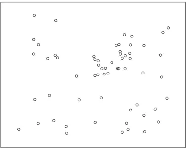
cases refer to individuals with a particular disease of interest, and controls refer to individuals with similar characteristics as cases but do not have the disease. When controls can be seen as a representative subset of population without the disease, comparison of the spatial distribution of the cases that of controls helps us identify spatial patterns in the cases distribution that are beyond what is merely reflective of the spatial distribution of the population. An example of case-control artificial data is shown in the Figure 1.2.
1.1.3
Aggregated Data
TYPES OF DATA 3
Figure 1.2: Spatial distribution of the observed cases (circles) and controls (dots) in Lancashire-UK data.
1.1.4
Space Time Data
KULLDORFF’S SPATIAL SCAN STATISTIC 4
=0 <0.013 0.013 to 0.026 0.026 to 0.047 >0.047
Rate
(a)
<0.2 0.2 to 0.5 0.5 to 0.9 0.9 to 0.95 >0.95
Population quantiles
(b)
Figure 1.3: Mapping spatial variations of Chagas disease in the State of Minas Gerais - Brazil by county during 2006: (a) disease rates map; (b) Population at risk map.
1.2
Kulldorff ’s Spatial Scan Statistic
SPATIAL CLUSTER INFERENCE 5
each region is Poisson distributed proportionally to its population. For each zone z, the number of observed cases is zC and the expected number of
cases under null hypothesis is zµ=zN(C/N), where zN is the population in
the zone z. Defining L(z) as the likelihood function under the alternative hypothesis and L0 as the likelihood function under the null hypothesis, it can be shown (Kulldorff, 1997) that the logarithm of the likelihood ratio, K(z) = log (L(z)/L0), for the Poisson model is given by:
K(z) =
Clog N C
+zClog
zC
zN
+ (C−zC) log
C
−zC
N −zN
if zC
zN
> C−zC N −zN
0 otherwise
(1.1) The function K is maximized over the chosen set Z of potential zones z, identifying the zone which constitutes the most likely cluster. Hence we have the test statistic, given by T = maxzK(z).
Given the definition above, it follows thatK(z) =K(zC,zN) is a function
of variables zC and zN. Assuming thatzC and zN take positive values, it is
trivial to note that K(zC,zN) satisfies the following property:
Property 1 Let zC/zN >(C−zC)/(N −zN). The function K(zC,zN) is
strictly increasing in the variable zC and strictly decreasing in the variable
zN.
1.3
Spatial Cluster Inference
PROSPECTIVE SPACE-TIME SCAN 6
the regions of the study area. The cases distribution, conditioned on the total number of cases, is made according a multinomial distribution where the probability of an individual become a case in any region is proportional to its population. Then the scan statistic is calculated for the most likely cluster given the simulated cases distribution. This procedure is repeated n times and the obtained scan statistic values are ranked (the value corresponding to the 95% quantile is the estimate of the critical value at a 5% significance level). Given the scan statistic value, T, of the observed cases map, the estimate of its p-value is nobs
n+ 1, where nobs is its ranking position among the n+ 1 values (where n is the number of simulated values).
1.4
Prospective Space-Time Scan
The Prospective Space-Time Scan (Kulldorff, 2001) considers all cylin-drical clusters in the space-time domain. All the possible circular windows in the space domain are taken as the bases of the cylinders to be considered. The study period is given by the time interval [Y1, Y2]. The likelihood for the observed data set is obtained as the maximum over all cylinders in the time interval [s, t] reaching the end of the study period, with Y1 ≤ s ≤ t = Y2. For the random data sets generated under null hypothesis, the likelihood is maximized over all cylinders for which Y1 ≤ s ≤ t ≤ Y2 and Ym ≤ t,
where Ym is the time instant in which the time periodic surveillance began,
STATE-OF-THE-ART 7
1.5
State-of-the-art
The spatial scan statistic (Kulldorff, 1997) constitutes the main statis-tic used for cluster detection, being employed, for instance, by the software packages SaTScan (Kulldorff,1999) to detect static circularly shaped disease clusters (Kulldorff & Nagarwalla, 1995). Recently, several attempts have been developed in order to relax the assumption of cluster circular shape.
(Sahajpal et al., 2004) used a genetic algorithm to find clusters shaped as
intersections of circles of different sizes and centers. The SaTScan approach has been extended to the case of elliptic shaped clusters (Kulldorffet al.,
2006), in this way allowing the detection of elongated clusters. Other meth-ods have also been proposed to detect connected clusters of irregular shape (Duczmal & Assun¸c˜ao,2004;Patil & Taillie,2004;Tango & Takahashi,2005;
Duczmal et al., 2006, 2008; Neill, 2008, 2010). The Static Minimum
Span-ning Tree (SMST) proposed by (Assun¸c˜ao et al., 2006) used a greedy algo-rithm to aggregate regions. The Flexibly Shaped (FS) spatial scan statistic
(Tango & Takahashi, 2005) made an exhaustive search of all possible
first-order connected clusters contained within a set encompassing the nearest k neighbors of a given region.
A key point for the construction of such methods for detection of ir-regularly shaped clusters is that, as the geometrical shape receives more degrees of freedom, some correction should be employed in order to compen-sate the increased flexibility, so avoiding the increase of false-positive errors
(Duczmal et al., 2006, 2007). This fact has been recognized since the early
study of elliptically shaped clusters (Kulldorffet al., 2006). These correc-tions were also treated in a multi-objective framework (Duczmal et al.,2008;
Duarte et al., 2010; Can¸cado et al., 2010). (Yiannakoulias et al., 2007)
pro-posed a topological penalty.
pres-STATE-OF-THE-ART 8
ence of those potential gaps is to limit the number of component areas of the cluster, e.g. allowing only clusters which are subsets of a circular zone of moderate maximum size.
Recently, methods have been proposed when point process data are avail-able. (Conley et al., 2005) proposed a genetic algorithm to explore a config-uration space of multiple agglomerations of ellipses in point data set maps, implemented in the software PROCLUDE. (Wieland et al.,2007) introduced a graph theoretical method for detecting arbitrarily shaped clusters based on the Euclidean minimum spanning tree of cartogram transformed case loca-tions, which is quite effective, but the cartogram construction step of this algorithm is computationally expensive and complicated. (Demattei et al.,
Chapter 2
Voronoi based scans for point
data sets
2.1
Motivation
Algorithms for the detection and inference of clusters are useful tools in etiological studies (Lawson et al.,1999) and in the early warning of infectious disease outbreaks (Duczmal & Buckeridge,2006;Kulldorff et al.,2005,2006,
2007; Neill, 2009). A spatial cluster is defined as a localized portion of the
domain containing a higher than average proportion of cases over controls, whose appearance is unlikely under the assumption that cases are randomly distributed in the population. Space-time clustersare defined as unexpected concentrations of disease cases in a time series sequence of geographical maps, and could potentially indicate an outbreak or epidemic, due to environmental or biological causes.
The mechanism behind the enhancement of the power of cluster detection methods when arbitrary shapes are considered can be described as:
• If the shape of the possible cluster was known a priori, the most power-ful method of detection would be to assume such a shape, and search for empirical clusters of that format. In this way, objects of other shapes
MOTIVATION 10
would be disregarded, and the statistics would be evaluated only over the legitimate cluster candidates.
• If the shape of possible clusters was not known a priori, considering a fixed shape would lead to two kinds of errors: either the true cluster would be included inside a greater cluster estimate of the assumed shape, or only a portion of the true cluster which coincides with the assumed shape would be considered. In both cases, the power of the method would be decreased due to such errors.
• An entropy-like argument is employed at this point: the relatively rare regular shapes that would represent a homogeneous formation of the cluster are considered better than the more numerous flexible irregular shapes, that represent a rather non-homogeneous cluster propagation.
• Within the multi-objective framework, there is no need to state pre-cisely the relative weight of the different shapes. The suitable balanc-ing of the minimization of shape flexibility and the maximization of the likelihood ratio of the existence of the cluster can be attained by a hypothesis test, which reveals a cluster estimate with minimal p-value. These developments related to flexible cluster shapes have been mostly performed for the static case only. The first motivation of this work is the concepts from the graph theory, applied to evaluate the set of potential clus-ters, for detecting arbitrarily shaped clusters based on the minimum spanning tree representation.
For the space-time case, the Prospective Space-Time Scan (Kulldorff,
DEFINITIONS AND METHODS 11
to inaccuracies in space-time cluster detection. This issue has been dealt in some references (Iyengar, 2005; Takahashi et al., 2008; Demattei & Cucala,
2011). See (Robertson & Nelson, 2010) for a review of space-time cluster detection software.
Our proposed methodology builds different graphs for each considered time interval. In this way, the flexibility that is necessary for dealing with the variation of the disease spread along the time dimension is obtained in a direct way.
2.2
Definitions and Methods
The idea of employing a Minimum Spanning Tree (MST) in order to char-acterize clusters has been already studied by (Assun¸c˜ao et al., 2006), in the context of area data sets. For dealing with point data sets, the application of the scan statistics requires a proper definition of disease case density related to each data point. As, clearly, a single sphere radius was not suitable for estimating the population density in all regions, due to the heterogeneity in the geographical distribution of population, a correction procedure was necessary. The procedure proposed by (Wieland et al., 2007) performed a non-linear cartogram transformation of the map, leading to a new map with an approximately homogeneous control population distribution. It should be noticed that this procedure is highly computing intensive.
DEFINITIONS AND METHODS 12
one. The computation of the Voronoi distance and all associated entities can be performed with efficient polynomial algorithms. Using the VMST, the computation of disease clusters in a fixed time coordinate can be performed very fast. In order to deal with space-time clusters, a simple procedure that connects the graphs of different time instants by the common nodes is em-ployed. The program was written in Dev C language.
2.2.1
Minimum spanning tree representation
We will use a Minimum Spanning Tree to represent a set of event data point and determine the subsets which potentially constitute a cluster.
In order to characterize point data set clusters, the Voronoi distance is defined. The population at risk consists ofN individuals in the space domain, divided into n disease cases and N − n controls. Consider the set P =
{(xi, yi) :i = 1, ..., N} ⊂R2, indicating the geographic location of the cases
and controls. For i = 1, ..., N the Voronoi cell v(i) consists of those points in R2
which are closer to (xi, yi) than to any other point in P. The Voronoi
diagram is formed by the collection of cells v(i), i= 1, ..., N.
Definition 1 (Voronoi distance) Let vij be the number of Voronoi cells
intercepted by the line segment joining the points (xi, yi) and (xj, yj)
(in-cluding the cells containing the points i and j). In this work we define the Voronoi distance between points i and j as δ(i, j) = vij−1. When the points
i and j occupy neighboring Voronoi cells, δ(i, j) = 1.
A geometric routine is used to compute the number of intersections of the segment linking two cases i and j with the edges of the Voronoi cells. If that segment intercepts tangentially a Voronoi cell, a potential problem may occur in the computation of δ(i, j). However, this problem occurs only rarely, supposing that the point coordinates follow a random pattern.
As an attempt to identify subsets of such a set that are likely to con-stitute a cluster, the following heuristic is employed here, (Xuet al., 2002;
Wieland et al., 2007): A nonempty subset S of D forms a candidate cluster
DEFINITIONS AND METHODS 13
maximum internal distance of S, where D−S is the subset of D removing all points of S. Formally, this can written as:
Let S = S1 ∪S2 be any partition and ρ represent the distance between two points of D. IfS ⊆D forms a cluster then
arg min
d∈D−S1
{min{ρ(d, s) :s∈S1}} ∈S2.
Hence, the potential cluster is a connected graph with tree structure, linking the disease cases in the space domain. Our algorithm builds a set of sub-trees of the minimum spanning tree of the complete graph of cases, defining a small set of potential space clusters. For example, considering the data points of the Figure 2.1 the points of the same cluster are connected with each other by short edges while long edges link cluster together.
VORONOI BASED SPATIAL SCAN 14
2.3
Voronoi based spatial scan
Formally, letD={ci} be the subset representing the disease cases where
each ci = (xi, yi) indicates its geographic location. We define a weighted
complete graph G(D) = (V, E) with vertex set V = {ci : ci ∈ D} and edge
setE ={(ci, cj) :ci, cj ∈D, i6=j}. Each edge (ci, cj)∈Ehas weight defined
by the Voronoi distance δ(i, j).
A minimum spanning tree (MST) of a weighted complete graphG(D) can be defined as a minimal set of edges of G(D) that connect all vertices with minimum total distance. The Voronoi Minimum Spanning Tree (VMST) of the weighted graphG(D) defined above is a spanning tree with the minimum total Voronoi distance. A set of discrete values characterizes the Voronoi dis-tance. This would cause the emergence of multiple solutions very often. This effect is eliminated by ordering the edges with identical Voronoi distances according to the Euclidean distance. This procedure ensures the following lemma, which is an extension of the result proposed by (Wielandet al.,2007):
Lemma 1 Assume that the Euclidean distance between any two points be-longing to the set P is different from any other distance between two points of the same set. Then the set of potential clusters are in one-to-one corre-spondence with connected components among all graphs Tw, with Tw defined
as the graph derived from VMST by deleting all edges having weight greater than w.
Proof: Define the order of descending weights w to the edges of VMST untied by Euclidean distance as discussed above. Hence, the proof follows the same way as performed in (Wieland et al.,2007), replacing the Euclidean distance by Voronoi distance.
The set of potential clusters may be quickly found from a VMST by using a greedy edge deletion procedure, improving and simplifying the strategy employed by the Density-Equalizing Euclidean MST method (Wielandet al.,
VORONOI BASED SPATIAL SCAN 15
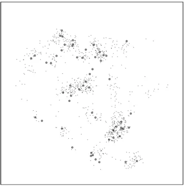
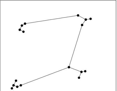
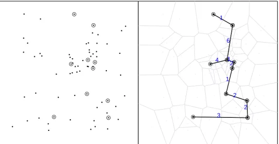
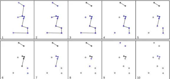
Figure 2.2 shows the spatial distribution of 70 coordinates, with 10 ob-served cases (circles) and 60 non-cases (dots) in an artificial data set and the associated Voronoi minimum spanning tree. Figure 2.3 shows a simple visualization of the greedy edge deletion procedure for the example above. The successive steps of edge deletion are represented, with the new cluster candidates shown in each iteration.
2
2 3
1
6
4 1
1 2
Figure 2.2: Left: spatial distribution of the 10 observed cases (circles) and 60 non-cases (dots). Right: corresponding Voronoi minimum spanning tree.
Given a case with geographic location ci = (xi, yi), consider the circle
C(ci, r) centered in the point (xi, yi), with radiusr. If the local density around
the point (xi, yi) is given by s individuals per unit area, then the expected
number of individuals inside the circle C(ci, r) is computed as sπr2. When
the radius r is expressed locally in units of the Voronoi distance as R, then the expected number of individuals inside C(ci, r) is simply πR2. Thus the
VORONOI BASED SPATIAL SCAN 16
1 2 3 4 5
6 7 8 9 10
Figure 2.3: Visualization of the greedy edge deletion procedure, in successive steps numbered from 1 to 10. Sub-graphs linking blue circles represent the new cluster candidates that appear in each iteration, and sub-graphs link-ing black circles represent cluster candidates that have already appeared in former steps.
Proposition 1 Consider a case dataset D and its corresponding VMST, denoted by V. Let TS be a connected subgraph of V whose nodes constitute
the set S, and denote byf(x) the local population density inx. For each case
ci ∈S let ωi be equal to the minimum weight of the edges that are incident to
ci in V andB=
S
C(ci, ωi/2). The local population of S can be approximated
by
Z
B
f(x)dx= 1 4
X
ci∈S
πω2
i.
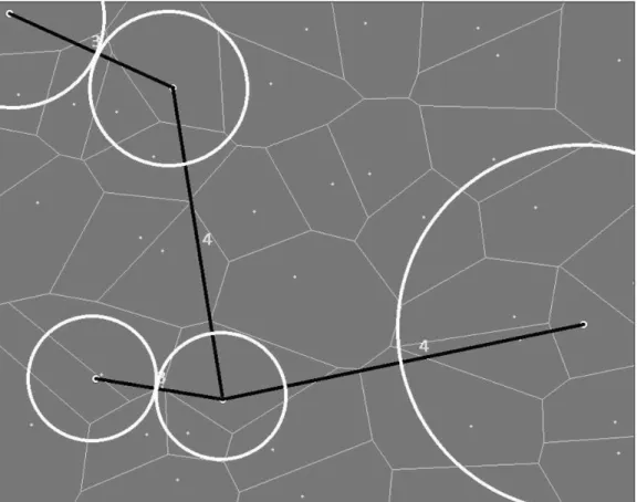
This defines a “region of influence” of the cluster S through the compo-sition of the regions of influence of each case, which are defined as circular regions, with radii ωi/2 chosen as large as possible, such that there is no
interference between neighboring circles in the VMST. An example is shown in Figure 2.4.
We further note that this definition is robust, in the following sense. Consider two situations: first, a case dataset D spread evenly in a map of control points, and second, a case dataset D′
VORONOI BASED SPACE-TIME SCAN 17
Figure 2.4: The “region of influence” of each individual case in an arbitrary map.
of the clusters associated to D is larger than the corresponding regions of influence associated with D′
, as we could expect.
We shall use this information to estimate the number of control individ-uals under the “region of influence” of each case individual, which in turn will allow the use of the scan statistic and also define a corresponding cluster finding algorithm employing a minimum spanning tree.
2.4
Voronoi based space-time scan
VORONOI BASED SPACE-TIME SCAN 18
temporal gap within the candidate cluster.
LetPT be the set of the geographic coordinates of theN−n controls and
the nT disease cases present in the interval time window given by T = [s, t],
wheres is the initial time andtthe final time of the interval T. The Voronoi diagram ofPT and the corresponding Voronoi distance is defined similarly to
the former procedure, in space coordinates only. For the space-time domain, let ti be the onset time of the disease for the i-th case, i = 1, ..., nT. Then,
establish connections linking only cases whose temporal distance is limited by τ.
Formally, let DT = {cti
i : i = 1, ..., nT} be the set of cases observed in
the interval T = [s, t], wheres ≤ti ≤t and (xi, yi) indicates the geographic
location for thecti
i case,i= 1, ..., nT. In this way, two observed casesctii, c tj
j ∈
DT will be connected if the temporal distance is such that |t
i−tj| ≤ τ.
We define a weighted complete graph Gτ(DT) = (VT, Eτ) with vertex set
VT = {cti
i : c
ti
i ∈ DT} and edge set Eτ = {(c ti
i , c
tj
j ) : c
ti
i , c
tj
j ∈ DT, i 6=
j,|ti−tj| ≤τ}. The weights are the usual Voronoi distances between points
(xi, yi) and (xj, yj).
The procedure is repeated for every time interval T = [s, t] such that Y1 ≤ s ≤ t = Y2, as seen in the Prospective Space-Time Scan section, building a different Voronoi based MST for each time interval T.
Chapter 3
Dynamic Programming based
Scan
3.1
Motivation
In general, the greatest difficulty of methods for detection of spatial clus-ters is to identify over all subsets of the data the subset that corresponds to the pattern of discrepancy. The evaluation of all subsets is computa-tionally infeasible for large dataset. Recently, several attempts have been developed in order to outline this problem. Many heuristics have appeared recently to compute approximate values that maximizes the logarithm of the likelihood ratio (Duczmal et al., 2009), other methods have made to reduce the search space (Duczmal et al.,2011;Wielandet al.,2007;Demattei et al.,
2007). Neill’s Fast Subset Scan (Neill, 2008) presented a significant advance in spatial methods for aggregated area maps, finding exactly the optimal irregularly spatial clusters.
In (Cancado,2009), the spatial cluster detection problem is formulated as
the classic knapsack problem. The problem can be modeled as abi-objective combinatorial optimization problem. The set of non-dominated solutions of the problem contains the solution that maximizes the logarithm of the
MULTI-OBJECTIVE OPTIMIZATION PROBLEM 20
hood ratio,K(z). In this work, a knapsack problem (unconstrained versions) is proposed.
We propose an exact algorithm based on dynamic programming, Geo-graphical Dynamic Scan, that empirically was able to solve instances up to large size within a reasonable computational time. The set of non-dominated solutions of the problem, computed efficiently, contains the solution that maximizes the logarithm of the likelihood ratio, K(z). The method allows arbitrary shaped clusters, which can be a collection of disconnected or con-nected regions, taking into account a geometric constraint. Note that this is not a serious disadvantage, provided that there is not a huge gap between its areas. Finding exactly the optimal irregularly spatial clusters, the method allows multiple clusters.
We present an empirical comparison of detection and spatial accuracy between our algorithm and the classical Kulldorff’s Circular Scan, using the data set of Chagas disease cases in puerperal women in Minas Gerais state, Brazil.
3.2
Multi-objective optimization problem
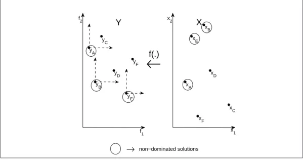
Multi-objective optimization deals with the problem of finding optimal solutions due to more than one objective function. A multi-objective opti-mization problem is formally defined as:
minf(x), f(x) = (f1(x), f2(x),· · · , fm(x))
subject to: x= (x1, x2,· · · , xn)∈X
(3.1)
in which x ∈ X ⊆ Rn is the decision variable vector, X is the optimization
parameter domain, Y ⊆Rm is the objective space, i.e. Y =f(X).
MULTI-OBJECTIVE OPTIMIZATION PROBLEM 21
the following relational operators:
u,v∈Rm
u≦v ⇐⇒ ui ≤vi, i= 1, . . . , m
u 6=v ⇐⇒ ∃i∈ {1, . . . , m}: ui 6=vi
u≤v ⇐⇒ u≦v and u6=v
These operators enable a well-defined definition of optimality in multi-objective optimization.
Definition 2 A feasible solutionx∗
∈Xis called optimal solution of a multi-objective optimization problem if there is no x∈X such that f(x)≤f(x∗
).
In that case f(x∗
) is called optimal value of the multi-objective optimization problem.
Given the multi-objective optimization problem (3.1), a decision vector
x dominates another decision vectorx′
and f(x) dominatesf(x′
) if and only if f(x)≤ f(x′
). An optimal solution is called non-dominated vector. In this way, the non-dominated set of solutions, or the Pareto-optimal set, P, is defined as:
P ={x∗
|∄x∈X:f(x)≤f(x∗
), x∈X}. (3.2)
SYSTEM AND METHOD 22 f 1 f2 y B y A y C yD y E y F
→ non−dominated solutions
X Y
←
f(.)x2 x 1 x F xA x B xD x E x C
Figure 3.1: Non-dominated solutions. Right: the Pareto-optimal set. Left: the Pareto front set.
3.3
System and Method
In this section we propose an algorithm to solve the problem of detecting clusters using dynamic programming.
Dynamic programming is a stage-wise search method suitable for opti-mization problems whose solutions may be viewed as the result of a sequence of decisions (Guptaet al.,2008). The most attractive property of this strat-egy is that during the search for a solution it avoids full enumeration by pruning early partial decision solutions that cannot possibly lead to opti-mal solution. The dynamic programming relies on a principle of optiopti-mality. This principle states that in an optimal sequence of decisions or choices, each subsequence must also be optimal.
3.3.1
Mathematical Formulation
The typical detection of spatial clusters problem (1.1) across the set Z of all possible zones, is reformulated, in the same way as done in (Cancado,
solu-SYSTEM AND METHOD 23
tions, and discards those that will not lead to optimal solutions.
Given a map with m regions, consider the binary variables x1, ..., xm,
where xi = 1 if the i-th region is present in the cluster and 0 otherwise. Let
ci andni denote the number of cases and population ofi-th region. Consider
the following unconstrained bi-objective combinatorial optimization problem:
min f(x) = C(x) =−
m
X
i=1
cixi, N(x) = m
X
i=1
nixi
!
s.t. x∈ {0,1}m
(3.3)
A non-dominated solution x = (xi, ..., xm) of the Problem (3.3) above,
represents a subset of regions (zone) of the map with number of cases|C(x)|
and population N(x).
The following proposition shows that is possible to find the maximum of the function K by solving Problem (3.3), see (Cancado, 2009).
Proposition 2 The set of non-dominated solutions of Problem (3.3) con-tains the solution that maximizes K.
Proof: Let P be the set of non-dominated solutions of Problem (3.3)
P ={x|∄x∗
∈ {0,1}m :f(x∗
)≤f(x), x∈ {0,1}m},
andx∗∗
the subset of regions of the map that maximizes the functionK, with number of cases |C(x∗∗
)| and population N(x∗∗
). We show that if x∗∗ /
∈ P
then it leads to a contradiction. Indeed, if x∗∗ /
∈ P then there exists a pair (C(x),N(x)) such thatC(x)≤C(x∗∗
) andN(x)≤N(x∗∗
), with at least one inequality being strict. Hence, as K satisfies the property1, it follows that:
1. If C(x)<C(x∗∗
) and N(x) =N(x∗∗ ) then K(C(x),N(x)) = K(C(x),N(x∗∗
))> K(C(x∗∗
),N(x∗∗ )); 2. If C(x) =C(x∗∗
) and N(x)<N(x∗∗ ) then K(C(x),N(x)) = K(C(x∗∗
),N(x))> K(C(x∗∗
),N(x∗∗ )); 3. If C(x)<C(x∗∗
) and N(x)<N(x∗∗ ) then K(C(x),N(x))> K(C(x∗∗
),N(x))> K(C(x∗∗
SYSTEM AND METHOD 24
All cases above implies that K(C(x),N(x)) > K(C(x∗∗
),N(x∗∗
)). This shows that if x∗∗
is the solution that maximizes the function K, then x∗∗
∈ P.
3.3.2
Dynamic programming algorithm
In this section, we introduce the dynamic programming approach, which is an adaptation of the Nemhauser-Ullman algorithm for the {0,1}knapsack problem (Nemhauser & Ullmann, 1969).
The algorithm that we use to solve Problem (3.3) can be regarded as a dynamic programming algorithm. In what follows, we present the theoretical background of the algorithm. Given a map withmregions and a random list enumerated of the regions, a zone of the map can be represented by a vector
x ∈ {0,1}m. Let sets Zi = {(C(x),N(x)) | x
k = 0,∀k > i, x∈ {0,1}m}
that represent all zones with at most i-th first regions (given a random list enumerated of the regions), i= 0, . . . , m. We callzi = (zi
C,ziN)∈ Zi a state.
The inclusion chain
{(0,0)}=Z0
⊆ Z1
⊆. . .⊆ Zm =Z
holds by definition of the sets Zi. Note that the states inZ =Zm represent
the image of the feasible solutions of Problem (3.3), i.e.{z= (zC,zN)∈ Z}=
{(C(x),N(x)) | x∈ {0,1}m}. Hence, we can naturally define the concept
of dominance between two states. We say that a state z = (zC,zN) ∈ Z
dominates a state z′ = (z′
C,z
′
N)∈ Z if (zC,zN) dominates (z
′
C,z
′
N).
Definition 3 A statez∈ Z is called extension of a statezi = (zi
C,ziN)∈ Zi,
i < m, if z = (zi
C−cj,ziN+nj) for some j ∈ {i+ 1, . . . , m}. If j = i+ 1,
the state z is called successor of zi, denoted by s(zi).
This notion of states matches the notion of zones.
SYSTEM AND METHOD 25 Population 780 789 241 403 96 131 942 803 575 59 234 353 821 15 43 168 649 731 647 450 Cases 8
26 8
2 12 10 32 12 6 9 15 20 10 5 12 8 13 27 18 17
Figure 3.2: An arbitrary map with 20 locations and its distribution of pop-ulation at risk and cases per location.
x1=(0, 1, 1, 1, 0, 0, 0, 0, 1, 0, ..., 0)
1
2 3
4 5 6 7 8 9 10 11 12 13 14 15 16 17 18 19 20
x2=(0, 0, 0, 1, 1, 1, 0, 1, 1, 0, ..., 0)
1
2 3
4 5 6 7 8 9 10 11 12 13 14 15 16 17 18 19 20
Figure 3.3: Different solutions mapped to same statez= (−42;2008)∈ Z9 .
the state z= (−42;2008) ∈ Z9
SYSTEM AND METHOD 26
state z= (−42;2008)∈ Z9
By the definition of a state successor and by construction we have the following recursion formula
Zi+1
=Zi∪
s(zi)|zi ∈ Zi , (3.4)
for i= 0, . . . , m−1.
We now state a theorem that justifies the use of dynamic programming in order to solve the problem of maximizing K.
Theorem 1 Let i < m. If z = (zC,zN) ∈ Zi is dominated by z′ =
(z′
C,z
′
N)∈ Zi, then there is an extension ofz
′
that will dominate any exten-sion of z.
Proof: Let z = (zC,zN) ∈ Zi be dominated by z′ = (z′C,z
′
N) ∈ Zi and let
the state ext(z) = (zC−cjz,zN+njz) ∈ Z denote an extension of z with
index jz ∈ {i+ 1, . . . , m}. Make the extensionext(z′) ofz′ defined by setting
jz′ = jz. It has to be shown that ext(z′) dominates ext(z). Because z is dominated by z′
, we get z′
C ≤zCand z′N ≤zN where at least one inequality
is strict. By definition of ext(z′
) and ext(z) the same values are added to
z′
C,z
′
N andzC,zN. Therefore, z′ dominateszimplies thatext(z′) dominates
ext(z).
The basic idea of the dynamic programming algorithm we are considering in the following is based on Theorem 1. The algorithm generates a sequence of sets of states Zi, i = 0, . . . , m. The set Zi+1
contains successors of the states in Zi but not those states that are dominated since they do not lead
to non-dominated states. We rewrite recursive formula Eq. (3.4) as follows:
Zi+1
= max
Zi∪
s(zi)|zi ∈ Zi
, (3.5)
for i= 0, . . . , m−1, where “max” denotes component-wise maxima.
GEOGRAPHICAL DYNAMIC SCAN 27
Problem (3.3). Since Z represents the image of the feasible solutions that maximizes the logarithm of the likelihood ratio, the algorithm test which one maximizes K function.
We showed that the dynamic programming algorithm allows to solve the unconstrained maximization of the functionKfor a spatial dataset. However, note that the unconstrained maximization over subsets of the Problem (3.3) is typically not sufficient to solve practical spatial detection problem. The method allows arbitrary shaped cluster, which can be a collection of regions with high likelihood that spreads randomly across the map. In the following section, we modify the dynamic programming algorithm in order to take into account a geometric constraint.
3.4
Geographical dynamic scan
The dynamic programming algorithm explained in the previous section is modified in order to consider ageographical proximity constraint. Consider a map with m regions and a fixed index k, 1 < k < m. For each region i, we define a centroidci, an arbitrary point in its interior,i= 1, ..., m. Letd(ci, cj)
be the Euclidean distance between any two centroids ci and cj of the map.
Then, for each region i, we define its geographical proximity Gi to be the
regioniand itsk−1 nearest neighbors regarding the distance to the centroid ci. We use the dynamic programming approach to find the non-dominated
solutions ofGi for each regioni. From the set of all non-dominated solutions
found for every region, we choose the one that is maximal with respect to functionK. Algorithm1introduces our approach to solve the classical spatial cluster detection problem.
Note that the geographical proximity constraint adopted is the same de-fined in the classical Kulldorff method, circular scan, see the Figure 3.4. However, assuming that the geographical proximity of a region i contains k regions, while the circular scan only evaluates k of the 2k subsets, the
geographical dynamic scan guarantees the optimal solution “evaluating” ef-ficiently the 2k subsets. Furthermore, another difference between the two
con-GEOGRAPHICAL DYNAMIC SCAN 28
Algorithm 1 Geographical dynamic scan algorithm 1. Let S =∅;
2. Define neighborhood size k and centroidsci for each regioni= 1, ..., m
of the map;
3. For each region i= 1, . . . , m
(a) LetGi be the geographical proximity for each region i= 1, ..., m;
(b) Let Sndi be the non-dominated set of Problem (3.3) using the
dynamic programming algorithm with input data Gi;
(c) S :=S∪Sndi;
(d) S :=N D(S), where N D define a non-dominated operator. 4. s:= max{K(S)};
5. Return s.
GEOGRAPHICAL DYNAMIC SCAN 29
Chapter 4
Results and Discussion
In this chapter we evaluate the numerical performance of Voronoi Based Scan and Geographical Dynamic Scan algorithms proposed in this work.
4.1
Evaluated Measures
A good detection method is that it is sensitive enough to detect a cluster when it actually exists. We will evaluate the efficiency of the algorithms in this thesis calculating their power.
Definition 4 (Power) The power of a statistical test measures the test’s ability to reject the null hypothesis when it is actually false.
In other words, the power of a hypothesis test is the probability of not com-mitting a type II error. We can estimate the power by Monte Carlo simu-lations, running the algorithm a large number of times in artificial settings, constructed so that there is the presence of a cluster. The maximum power a test can have is 1, the minimum is 0. Ideally we want a test to have high power, close to 1.
We also use the measures of sensitivity and positive predicted value (ppv) that serve to evaluate the quality of the cluster detection process. The mea-sures were defined differently according to the form of spatial data evaluated.
NUMERICAL TESTS 31
For the aggregated spatial data, the sensitivity and positive predicted value (ppv) are defined in the terms of the population size as
Sensitivity = P op(Detected Cluster∩Real Cluster) P op(Real Cluster)
P P V = P op(Detected Cluster∩Real Cluster) P op(Detected Cluster)
For case-control data spatial set, let {X1, X2, . . . , Xn} be random
vari-ables that denote the spatial coordinates of n cases observed in the data set. The sensitivity and positive predicted value are defined as
Sensitivity = Pn
i=11(Xi ∈Detected Cluster∩Real Cluster) Pn
i=11(Xi ∈Real Cluster)
P P V = Pn
i=11(Xi ∈Detected Cluster∩Real Cluster) Pn
i=11(Xi ∈Detected Cluster) where 1(.) is the indicator function.
Using artificial clusters, the measures of power, sensitivity and positive predicted value of the algorithms are estimated. In each scenario a relative risk equal to 1.0 was set for every region (considering aggregated spatial data) and every control (considering case-control spatial data) outside the real cluster, and greater than 1.0 and identical otherwise. The relative risks for each cluster are defined such that if the exact location of the real cluster was known in advance, the power to detect it would be 0.999 (Kulldorffet al.,
2003).
4.2
Numerical Tests
NUMERICAL TESTS 32
4.2.1
Voronoi Based Scan
In this section we present a set of numerical results. The Voronoi Based Scan (VBScan) was compared numerically with the elliptic version of the spa-tial scan and prospective space-time scan (Kulldorff et al., 2006; Kulldorff,
2001), according to power of detection, sensitivity and positive predictive value.
In the first set of simulations, we evaluated only the spatial structure of the proposed algorithm.
A verification for purely spatial clusters
The Voronoi based method, in its purely spatial setting, is applied for the well known data set of residential locations of larynx and lung cancer cases of the Chorley-Ribble area in Lancashire-UK, from 1973 to 1984. The 917 lung cancer cases are used as controls for the 57 larynx cancer cases (see http://cran.r-project.org/web/packages/splancs/splancs.pdf - pag. 55). In Figure4.1the spatial distribution of the observed cases (circles) and controls (dots) is shown on the left, and the Voronoi minimum spanning tree is shown on the right, with the Voronoi cells in the background. The elliptic spatial scan is also run as comparison. The p-values associated to the two scans are computed based on 9,999 Monte-Carlo simulations under the null hypothesis. The most likely clusters found in both runs are identical, consisting of the five cases (triangles) of Figure4.1. Table4.1 shows the likelihood values, number of cases, p-values and running times for both scans. The set of possible elliptic clusters forms a more restrictive space of configurations than the set of of irregularly shaped clusters; not surprisingly, the elliptic scan p-value is smaller than the VBScan p-value, because the five cases in the most likely cluster fit very well inside an elongated ellipse.
NUMERICAL TESTS 33
Figure 4.1: Left: Spatial distribution of the observed cases (circles) and con-trols (dots) in Lancashire-UK and the most likely cluster (triangles). Right: associated Voronoi minimum spanning tree.
Table 4.1: Comparisons spatial clusters detection of the cancer in Lancashire, match values to elliptic scan and VBScan methods.
Method LLR cases p-value CPU-Time(sec.) Elliptic Scan 14.4049 5 0.0089 896
VBScan 10.8357 5 0.0470 449.5
in Figure 4.2, aggregate spatial areas:
1. A circular shaped cluster was simulated with radius equal to 0.195. 2. A “T-2D”-shaped cluster was simulated with zone T =T1∪T2 where
T1 = [0.2,0.4]×[0.5,0.8], T2 = [0.0,0.6]×[0.8,0.9].
3. An “L-2D”-shaped cluster was simulated with zoneL=L1∪L2 where L1 = [0.2,0.4]×[0.5,0.8], L2 = [0.2,0.8]×[0.8,0.9].
NUMERICAL TESTS 34
circular shaped "L" shaped
"T" shaped
Figure 4.2: Three alternative artificial spatial clusters.
power, sensitivity an PPV were computed for the most likely cluster in each replication.
Table 4.2 shows the results. The power and PPV values are slightly higher for the elliptic spatial scan than for the Voronoi based method but the sensitivity is lower for the elliptic scan. In addition, the Voronoi based method requires less computational time for point data set compared to the elliptic scan statistic.
By Proposition 1, we attached a ball of radius ωi/2 to each case ci
be-longing to the cluster S. The value ωi was chosen as the minimum weight
of the edges that are incident to ci in the VMST. An alternative definition
may use the average (or even the median) of the weights of the edges that are incident to ci, instead of the minimum value of the weights. We have
NUMERICAL TESTS 35
Table 4.2: Power, positive predicted value and sensitivity comparisons for shaped spatial clusters
Power Sensitivity PPV
shape of
cluster Elliptic VBScan Elliptic VBScan Elliptic VBScan Circle 0.8400 0.7963 0.7257 0.8199 0.8347 0.7871 “T-2D” 0.7320 0.7067 0.5508 0.7270 0.7837 0.7398 “L-2D” 0.7206 0.6696 0.5501 0.7144 0.7740 0.6932
original definition using the minimum value of the weights, see Table 4.3. This is a good indication that proposed definition of local population of the cluster is stable.
Table 4.3: Power, positive predicted value and sensitivity comparisons for alternatives values of ωi.
shaped
ωi cluster Power Sensitivity PPV
minimum Circle 0.7004 0.8260 0.7771 edge weight “T-2D” 0.5910 0.7326 0.7263 “L-2D” 0.5703 0.7248 0.6801 average Circle 0.7963 0.8196 0.7873 edge weight “T-2D” 0.7075 0.7278 0.7404 “L-2D” 0.6716 0.7152 0.6932 median Circle 0.7921 0.8149 0.7888 edge weight “T-2D” 0.6982 0.7225 0.7424 “L-2D” 0.6705 0.7112 0.6970
Analysis of the Voronoi based space-time scan
pro-NUMERICAL TESTS 36
cess, and the time of occurrence of the events following a discrete uniform distribution.
The Voronoi based method was compared to the prospective elliptic space-time scan statistic. Three alternative models of space-time clusters with different shapes were simulated. The three space-time cluster zones, as shown in Figure 4.3, aggregate spatial areas in consecutive time coordinates: 1. A cylinder shaped cluster was simulated with radius of the circular base
and height equal to 0.198 and [3,6], respectively.
2. A cone shaped cluster was simulated as a frustum of a cone. The radius of lower and upper circular base were equal to 0.115 and 0.265, respectively. The time window was equal to [3,6].
3. An “L-3D”-shaped cluster was simulated with zoneL=L1∪L2 where L1 = [0.3,0.7]×[0.3,0.7]×[3,4], L2 = [0.484,0.7]×[0.3,0.7]×[5,6]. Table 4.4 presents the resulting average power, sensitivity and PPV for 10,000 replications of each one of the three cluster models obtained with the VBScan and Elliptic PST algorithms. For all three space-time clusters, the power of detection of the VBScan was higher than the power of the Elliptic PST. This also occurs for PPV and Sensitivity. The results found in the three measures evaluated for “L-3D”-shaped cluster show the greater flexibility of VBScan, compared with Elliptic PST method.
Table 4.4: Power, sensitivity and positive predicted value comparisons for the three alternatives space-time clusters.
Power Sensitivity PPV
shaped