Data-driven inference for the spatial scan statistic

M E T H O D O L O G Y

Open Access

Data-driven inference for the spatial scan statistic

Alexandre CL Almeida

, Anderson R Duarte

, Luiz H Duczmal

, Fernando LP Oliveira

and Ricardo HC Takahashi

Abstract

Background:Kulldorff_’s spatial scan statistic for aggregated area maps searches for clusters of cases without specifying their size (number of areas) or geographic location in advance. Their statistical significance is tested while adjusting for the multiple testing inherent in such a procedure. However, as is shown in this work, this adjustment is not done in an even manner for all possible cluster sizes.

Results:A modification is proposed to the usual inference test of the spatial scan statistic, incorporating additional information about the size of the most likely cluster found. A new interpretation of the results of the spatial scan statistic is done, posing a modified inference question: what is the probability that the null hypothesis is rejected for the original observed cases map with a most likely cluster of size k, taking into account only those most likely clusters of size k found under null hypothesis for comparison? This question is especially important when the p-value computed by the usual inference process is near the alpha significance level, regarding the correctness of the decision based in this inference.

Conclusions:A practical procedure is provided to make more accurate inferences about the most likely cluster found by the spatial scan statistic.

Background Introduction

Spatial cluster analysis is considered an important tech-nique for the elucidation of disease causes and epide-miological surveillance [1]. Kulldorff_’s spatial scan statistic, defined as a likelihood ratio, is the usual mea-sure of the strength of geographic clusters [2,3]. The cir-cular scan [4], a particir-cular case of the spatial scan statistic, is currently the most used tool for the detec-tion and inference of spatial clusters of disease.

The spatial scan statistic considers a study region A

divided into m areas, with total population Nand C

total cases. A zone is any collection of areas. The null hypothesis assumes that there are no clusters and the cases are uniformly distributed, such that the expected number of cases in each area is proportional to its population. A commonly used model assumes that the number of cases in each area is Poisson distributed pro-portionally to its population. Let cz be the number of

observed cases andnzbe the population of the zonez.

The expected number of cases under null hypothesis is

given byμz=C(nz/N). The relative risk of zisI(z) =cz/ μzand the relative risk outsidezisO(z) = (C- cz)/(C

-μz). IfL(z) is the likelihood function under the

alterna-tive hypothesis andL0 is the likelihood function under

the null hypothesis, the logarithm of the likelihood ratio for the Poisson model is given by:

LLR(z) = log

L(z)

L0

=

czlog(I(z)) + (C−cz) log(O(z)) ifI(z)>1

0 otherwise.

(1)

LLR(z) is maximized over the chosen set Zof potential zonesz, identifying the zone that constitutes themost likely cluster(MLC). A derivation of this model can be

found in [2]. When the setZ contain the zones defined

by circular windows of different radii and centers,

max-zÎZLLR(z) is the circular scan statistic. Other possible

choices for Zinclude the set of elliptic clusters [5], or even the set of irregularly shaped connected clusters [6,7].

The statistical significance of the original MLC of observed cases must be calculated employing Monte Carlo simulations to build an empirical distribution of

the obtained maxzÎZ LLR(z) values under null

* Correspondence: duczmal@est.ufmg.br

3

Department of Statistics, Universidade Federal de Minas Gerais, Campus Pampulha, Belo Horizonte/MG, Brazil

Full list of author information is available at the end of the article

hypothesis [8], because its analytical expression is gener-ally not known. Simulated cases are randomly distribu-ted over the study region such that each area receives, on average, a number of cases proportional to its popu-lation. The statistical significance of the original MLC of observed cases is tested comparing its LLR value with LLR values of the corresponding MLCs obtained for each Monte Carlo replication. In each one of those replications, the MLC will be chosen in the set of circu-lar clusters of every possible size centered on every area of the study region, meaning that the LLR(z) value is the only selected feature used to compare the original MLC with the random ones under null hypothesis. The scan statistic is then computed for the MLC. This pro-cedure is repeatedBtimes, obtaining the empirical dis-tribution of the maxzÎZ LLR(z) values. Let Y be the

number of times that those values are greater than the

LLRof the original MLC of observed cases. The p-value

of the original MLC is computed as (Y + 1)/B. In the following, the empirical distribution of theB obtained maxzÎZLLR(z) values under null hypothesis for circular clusters will be called thescan empirical distribution.

The statistical significance of the spatial scan statistic is done without pre-specifying the number of areas or the location of the most likely clusters, while adjusting for the multiple testing inherent in such a procedure. However, this adjustment is not done in an even man-ner for all possible cluster sizes, as will be shown later. The usual inference process compares the most likely cluster of observed cases with the all the circular most likely clusters of every possible size centered on every area of the study region. In this work it is presented a modification to the usual inference test of the spatial scan statistic: the observed most likely cluster found,

with k areas, will be compared with only those most

likely clusters of size kfound in the randomized maps

under the null hypothesis.

Gumbel approximations

Through extensive numerical tests it was shown [9] that, under null hypothesis, the scan empirical distribution for circular clusters is approximated by the well-known Gumbel distribution

f(x) =θ−1exp{−exp[(x−µ)/θ]−(x−µ)/θ}

with parameters μ (mode) and θ (scale). Using this

semi-parametric approach, the spatial scan distribution may be estimated using a much smaller number of Monte Carlo replications. For example, computing the maxzÎZLLR(z) values under null hypothesis for only 100 random maps, and obtaining their average and variance to calculate the mode and scale parameters, a semi-parametric Gumbel distribution is obtained, as accurate

as a purely null empirical distribution produced afterB = 10000 random Monte Carlo replications [9].

Methods

One could be concerned with the fact that it should be more appropriate to compare the original MLC only with those MLCs of null hypothesis replicated maps that resemble as much as possible the original cluster, in terms of size, population and geographic location. An extreme instance of this situation would require that the comparison clusters are picked only among those (rarely occurring) random replications for which the MLCs are exactly the same as the original MLC. However, this task is computationally unfeasible, because an enormous number of replications is needed in order to select a siz-able number of random simulations for which the simu-lated MLCs coincide with the original MLC. Therefore, those requirements must be somewhat relaxed. Request-ing that the population is the same (regardless of other factors) may also be difficult, especially for maps with highly heterogeneous populations. A possibility then is to allow different location centers and populations, but requesting that the number of areas in the cluster is the same.

Empirical distributions

The spatial scan statistic was designed to adjust for the multiple testing when evaluating clusters of different sizes and locations. This adjustment implicitly supposes that the scan distribution doesn’t change when restricted for any given fixed cluster size. As will be shown, this assumption may not be true. Define scankas the

empiri-cal distribution obtained from the scan empiriempiri-cal distri-bution which considers only clusters of size k. It is also show that the Gumbel semi-parametric approach could be extended to the scankdistributions.

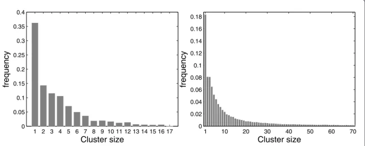
Frequency of cluster sizes

This subsection begins with two examples of maps with real data populations. The first map consists of 34 municipalities in the neighborhood of Belo Horizonte city in Brazil, with 6, 262 homicides cases during the 1998-2002 period, for a total population of 4, 357, 940 in 2000. The second map consists of 245 counties in 10 states and the District of Columbia, in the Northeastern U.S., with 58,943 age-adjusted deaths in the period from 1988 to 1992, for a population at risk of 29,535,210 women in 1990 [5].

typical examples of aggregated area maps, the fre-quency of cluster sizes varies widely; clusters of very small size are much more common. This means that the shape of the scan empirical distribution depends mostly on the smallest cluster size. Consequently, the decision process about the significance of the original MLC of observed cases relies mainly on the behavior of very small clusters, regardless of its size. One could argue that this feature, in itself, should not represent a problem if it could be guaranteed that the scank

distri-butions were nearly identical for every value of k.

However, as is shown in the next subsection, there are

significant differences between the various scank

distributions.

The Gumbel adjusted scan_kdistributions

As was done before for the empirical scan distribution, the Gumbel approximation for the scank distribution is

defined as the Gumbelk distribution. It was verified

experimentally that this adjustment was adequate, for all cluster sizes in several different maps.

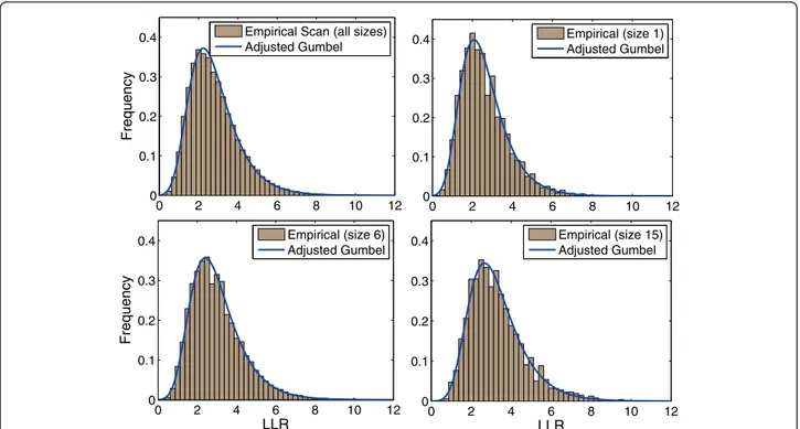
For the Belo Horizonte map, Figure 2 shows the scank

distributions taken from 1, 000, 000 Monte Carlo simu-lations and their respective Gumbelkadjusted

distribu-tions, forkvalues 1, 6 and 15.

Similarly, the same procedure was performed consid-ering the map of the Northeastern US, forkvalues 1, 20 and 80 as seen in Figure 3.

From the results of the 1, 000, 000 Monte Carlo simu-lations for the map of Belo Horizonte metropolitan area, it was observed that the critical values for the Gumbelk

distributions increase monotonically as the index k

increases from 1 to the maximum value 17. The Gumbel

adjusted distribution and the Gumbelkdistributions for

k= 1, 6 and 15 are displayed in the same graph on the

left of Figure 4. The a= 0.05 critical values for the four corresponding distributions are also shown.

For the Northeastern US map, similar results were observed when the Gumbel adjusted distribution and the Gumbelkdistributions fork= 1, 20 and 80 were put

together in the graph on the right of Figure 4, with the corresponding a= 0.05 critical values.

Those two examples show that the Gumbelk

distribu-tions change steadily with the size k, and are signifi-cantly different from the Gumbel adjusted distribution including all cluster sizes.

Data-Driven Inference

In its original formulation, the circular scan calculates the significance of the most likely cluster based on the fol-lowing question:“Given that the candidate cluster found hasLLR=x, what is the probability of finding a most likely cluster under the null hypothesis withLLR>x?_”

As will be seen in this section, clusters of small size constitute the majority among the MLCs found, and have the highest influence in the determination of the scan empirical distribution. In the situation when the MLC has large size, its inference will be made basically by the behavior of small clusters.

In this section it is proposed to use the information about the size of the observed MLC in the inference test. In this case, the following question is formulated: “Given that the candidate most likely cluster hasLLR= x and containskareas, what is the probability to find, under the null hypothesis, a cluster formed bykregions withLLR > x?”

1 2 3 4 5 6 7 8 9 10 11 12 13 14 15 16 17 0

0.05 0.1 0.15 0.2 0.25 0.3 0.35 0.4

Cluster size

frequency

1 10 20 30 40 50 60 70

0 0.02 0.04 0.06 0.08 0.1 0.12 0.14 0.16 0.18

Cluster size

frequency

Figure 1Frequency distribution of the sizes of the most likely clusters found underH0, with 1,000, 000 Monte Carlo replications, for

0 2 4 6 8 10 12 14 0

0.1 0.2 0.3 0.4

LLR

Empirical (size 80) Adjusted Gumbel

0 2 4 6 8 10 12 14

0 0.1 0.2 0.3 0.4

LLR

Frequency

Empirical (size 20) Adjusted Gumbel

0 2 4 6 8 10 12 14

0 0.1 0.2 0.3

0.4 Empirical (size 1)

Adjusted Gumbel

0 2 4 6 8 10 12 14

0 0.1 0.2 0.3 0.4

Frequency

Empirical Scan (all sizes) Adjusted Gumbel

Figure 3The scankdistributions taken from 1, 000, 000 Monte Carlo simulations in the Northeastern US map, and heir respective

Gumbelkadjusted distributions, fork= 1, 20 and 80.

0 2 4 6 8 10 12

0 0.1 0.2 0.3 0.4

Frequency

Empirical Scan (all sizes) Adjusted Gumbel

0 2 4 6 8 10 12

0 0.1 0.2 0.3

0.4 Empirical (size 1) Adjusted Gumbel

0 2 4 6 8 10 12

0 0.1 0.2 0.3 0.4

LLR

Frequency

Empirical (size 6) Adjusted Gumbel

0 2 4 6 8 10 12

0 0.1 0.2 0.3 0.4

LLR

Empirical (size 15) Adjusted Gumbel

Figure 2The scankdistributions obtained from 1, 000, 000 Monte Carlo simulations in the Belo Horizonte etropolitan area map, and

The proposal of this paper takes into account the cluster size, as follows: given that the circular scan

has found the observed MLC with k regions, then its

statistical significance is still obtained through Monte Carlo simulations, but selecting only those

replica-tions for which the MLC solureplica-tions have exactly k

areas. The empirical scan distribution that considers

MLC solutions of any size is replaced by the scank

empirical distribution with MLCs of size exactly equal tok.

However, when the p-value is much smaller or much larger than the significance level a, there is no change in the decision to reject, or not, the null hypothesis. Thus, only the more difficult decision process is of interest, namely when the computed p-value is close to the significance levela.

Results

In this section, numerical experiments are made showing that the proportions of rejections of the null hypothesis differ noticeably, by employing the usual critical value, compared with using the data-driven critical values. It is also shown that the computa-tional cost of estimating the data-driven critical value may be reduced through the use of a simple interpolation.

Critical values variability

To assess the variability in the estimation of the critical

values of each scank distribution, another batch of

Monte Carlo simulations was conducted. First a set S0

of 1, 000, 000 random replications under null hypothesis was computed and the usual critical valuev0was

deter-mined for thea= 0.05 significance level employing the empirical scan distribution. Next, for every value of size kthe empirical scankdistribution and the corresponding

critical value vk at the a = 0.05 significance level was

determined.

Following, 100 sets Si,i= 1, ..., 100 of 1, 000, 000

ran-dom replications each were computed under null hypothesis. For each set Siand for every value of size k

the corresponding empirical scank distribution for the

set Si was computed, and called scanki. The proportion

pki(respectivelyqki) of computed MLCs’LLR values

lar-ger than v0 (respectively vk) in the distribution scanki

was obtained, for every value kand i = 1, ..., 100. For every value of k, the 100 valuespki (respectivelyqki), for

i = 1, ..., 100, were used to build the 95% confidence

intervalsUk (respectivelyDk), thus estimating the error

bar in the proportion of rejection of the null hypothesis through the usual (respectively data-driven) inference process.

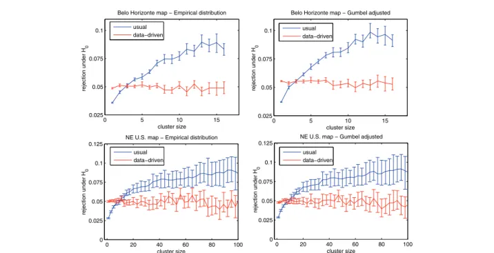
The graphs on the left part of Figure 5 show the results using the data for the Belo Horizonte metropoli-tan area (above) and the US Northeastern map (below). The graphs in blue color show the error bars for the 95% usual non parametric confidence intervals Uk, for

every sizek, showing the average and the variability of the proportion of likelihood ratios higher than the

usual critical value v0, which employs MLCs of every

size k in the empirical scan distribution. Otherwise,

the graphs in red color show the error bars for the

0 2 4 6 8 10

0 0.05 0.1 0.15 0.2 0.25 0.3 0.35 0.4

LLR

frequency

2 4 6 8 10 12

0 0.05 0.1 0.15 0.2 0.25 0.3 0.35 0.4

LLR

size 1 distribution size 6 distribution size 15 distribution

usual Scan size 1 distribution size 20 distribution size 80 distribution

Figure 4The Gumbel adjusted distribution and the Gumbelkdistributions for several values ofk, with their respectivea= 0.05

95% data-driven non-parametric confidence intervals Dk, for every sizek, showing the average and variability

of the proportion of likelihood ratios higher than the data-driven critical valuesvk, which separates MLCs of

different sizes k into their corresponding empirical

scank distributions. For each dataset, the blue and red

error bars are clearly distinct, showing the differences between the usual and data-driven inferences. A simi-lar procedure was used to compute the 95% non para-metric confidence intervals for the corresponding adjusted Gumbelk distributions, instead of the

empiri-cal scank distributions. The corresponding sets of error

bars for the Gumbel adjusted distributions are dis-played in the right part of Figure 5, for the Belo Hori-zonte metropolitan area (above) and the US Northeastern map (below). From Figure 5 it is noted that the values obtained through the data-driven infer-ence are substantially closer to the 0.05 level, for both

maps. The usual approach’s rejection rate of about

0.03 to 0.04 for small clusters means it is not rejecting enough small clusters, thus returning too many false positives. The opposite happens for large clusters.

Practical evaluation of critical values

From a practical viewpoint, one could be concerned with the large number of simulations necessary to obtain a reasonable number of replications for which their MLCs have exactly the size of the observed MLC,

in order to estimate the data-driven critical value. It is

shown that, through interpolation of the vk critical

values for the values of size k close to the observed

MLC size, a fairly small number of replications produce a consistent critical value estimate.

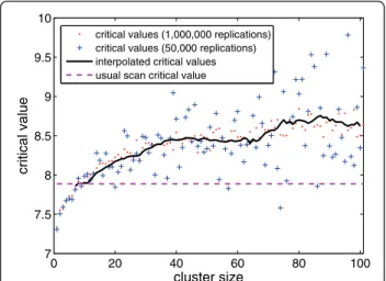
Figure 6 shows the data-driven critical values for the

Northeastern US map for the k size values, using

1,000,000 (respectively 50,000) replications, displayed as red dots (respectively blue crosses). The solid black curve represents the moving average, of window size 20, of the critical values for each size k> 10 using the 50,000 replications set (blue crosses). As can be seen in Figure 6, the moving averages fall approximately within the 1,000,000 set’s obtained critical values (red dots). The horizontal dashed line indicates the usual critical value. This very simple scheme is thus suffi-ciently stable, allowing the use of a small number of Monte Carlo replications to estimate the data-driven critical values. For smaller maps (as the Belo Horizonte metropolitan area map), the computational effort is lower, and the data-driven critical values are easier to calculate.

Conclusions

The classical inferential process used in the inference of spatial clusters employing Kulldorff_’s Spatial Scan statis-tic considers all the most likely clusters found in Monte Carlo replications under the null hypothesis in order to

0 5 10 15

0.025 0.05 0.075 0.1

cluster size

rejection under H

0

Belo Horizonte map − Empirical distribution

0 5 10 15

0.025 0.05 0.075 0.1

cluster size

rejection under H

0

Belo Horizonte map − Gumbel adjusted

0 20 40 60 80 100 0

0.025 0.05 0.075 0.1 0.125

cluster size

rejection under H

0

NE U.S. map − Empirical distribution

0 20 40 60 80 100 0

0.025 0.05 0.075 0.1 0.125

cluster size

rejection under H

0

NE U.S. map − Gumbel adjusted usual

data−driven

usual data−driven

usual data−driven

usual data−driven

Figure 5The proportion of null hypothesis rejection, for the empirical (left) and Gumbel adjusted (right) distributions, for the Belo

build the empirical distribution of the likelihood ratio, regardless of cluster size and location. A potential disad-vantage of this approach is the implicitly assumed inde-pendence of the log likelihood ratio distributions, when restricted to the various sizes of the most likely cluster found. It was shown, through numerical experiments, that this assumption is not true for commonly occurring real data maps. Given that the observed most likely clus-ter has size k0, that means that the classical inference

process computes its significance based on the behavior of most likely clusters whose sizes are different fromk0.

In this work an alternative was proposed, the data-dri-ven inference, which takes into account only those most likely clusters found whose size is identical to the size of the observed most likely cluster. This approach employs a more specific comparison, thus avoiding that the beha-vior of clusters of very small size are used to decide if a large observed most likely cluster is considered signifi-cant, for example.

As the number of most likely clusters of certain speci-fic size found in randomized maps is smaller than the total number of Monte Carlo replications, a concern may arise that the computational effort to compute the significance with the data-driven inference process should be very high. However, it was shown that using the Gumbel semi-parametric approach and simple inter-polation techniques this effort could be mitigated. How many simulations are necessary to provide an acceptable confidence interval for the critical values for each value of size k? It would be very difficult to find a simple for-mula fitted for every kind of map. Given a particular map, it is suggested to apply the method described in

the _“Practical evaluation of critical values_”section, run-ning sequentially several sets of simulations with an increasing number of Monte Carlo replications, and waiting for the interpolated critical values curve to numerically stabilize.

For each value of size kthere are different distribu-tions of empirical values; in all the studied examples, the overall shape of those distributions varies smoothly as kvaries, and it even seems reasonable to conjecture that their averages increase monotonically as the value

of kincreases. However it is plausible to imagine an

hypothetical situation where those changes become abrupt with the variation ofk, characterizing instability of the null hypothesis. This instability should impact even more the usual inference, because the relative importance of the different values of k would not be identified, as was done in the present analysis. This kind of situation has not yet been experienced, although, and the experiments of the previous section may serve to assess that kind of instability in a particu-lar map.

It should be stressed that the present paper’s strategy of employing the size (number of areas inside the clus-ter) as the criterion to compare the most likely clusters is still subject to bias due to the heterogeneous popula-tion distribupopula-tion. A solupopula-tion for this problem should be the use of both variables, size and population, which would be very expensive, as discussed before.

The proposed method is more useful when the com-puted p-value using the classical inference is close to

the a significance level, otherwise there will be no

change in the decision process. In this situation, it is recommended that the data-driven inference should be performed, especially when the observed most likely cluster has relatively large size.

Numerical experiments were also performed using the data-driven inference for space-time cluster detection, considering not only the number of areas inside the cluster, but also the length of the time interval of the cylinders [10]. Preliminary results suggest that the differ-ences in the critical values are even more pronounced than in the purely spatial setting.

The data-driven inference could be applied to case/ controls point data set clusters, taking into account the number of cases and the population inside the clusters. There are three options to consider for the data-driven inference in this type of dataset, namely those based on the number of cases, population, or both. When based on the number of cases, provided that the number of cases is small, the data-driven inference follows the same lines of the present paper. Otherwise, when the number of cases is large or when the data-driven infer-ence is based on the population, some kind of interpola-tion scheme should be used.

0 20 40 60 80 100

7 7.5 8 8.5 9 9.5 10

cluster size

critical value

critical values (1,000,000 replications) critical values (50,000 replications) interpolated critical values usual scan critical value

Figure 6Data-driven critical values for the Northeastern US

Another extension should consider irregularly shaped clusters [11] instead of circular clusters. These ideas will be discussed in a future work.

Acknowledgements

We thank the editor and four reviewers for their thoughtful comments. We are grateful to Martin Kulldorff for his comments. The authors acknowledge the support of the Brazilian agencies Capes, CNPq and Fapemig.

Author details

1_{Campus Alto Paraopeba, Universidade Federal de São João del Rei, Ouro}

Branco/MG, Brazil.2_{Department of Mathematics, Universidade Federal de}

Ouro Preto, Ouro Preto/MG, Brazil.3_{Department of Statistics, Universidade}

Federal de Minas Gerais, Campus Pampulha, Belo Horizonte/MG, Brazil.

4_{Department of Mathematics, Universidade Federal de Minas Gerais, Campus}

Pampulha, Belo Horizonte/MG, Brazil.5Graduate Program in Electrical Engineering, Universidade Federal de Minas Gerais, Campus Pampulha, Belo Horizonte/MG, Brazil.

Authors’contributions

All the authors contributed to the methodology used in the study, wrote the necessary computer programs, conducted the simulations and data analysis, and drafted the manuscript. All authors have read and approved the final manuscript.

Competing interests

The authors declare that they have no competing interests.

Received: 4 June 2011 Accepted: 2 August 2011 Published: 2 August 2011

References

1. Lawson A:Statistical methods in spatial epidemiology.InLarge scale: surveillance.Edited by: Lawson A. London: Wiley; 2001:197-206. 2. Kulldorff M:A Spatial Scan Statistic.Communications in Statistics: Theory

and Methods1997,26(6):1481-1496.

3. Kulldorff M:Spatial Scan Statistics: Models, Calculations, and Applications.

InScan Statistics and Applications.Edited by: Balakrishnan N, Glaz J. Birkhäuser; 1999:303-322.

4. Kulldorff M, Nagarwalla N:Spatial disease clusters: detection and inference.Statistics in Medicine1995,14:799-810.

5. Kulldorff M, Huang L, Pickle L, Duczmal L:An elliptic spatial scan statistic.

Statistics in Medicine2006,25:3929-3943.

6. Duarte AR, Duczmal L, Ferreira SJ, Cancado ALF:Internal cohesion and geometric shape of spatial clusters.Environmental and Ecological Statistics

2010,17:203-229.

7. Cancado ALF, Duarte AR, Duczmal L, Ferreira SJ, Fonseca CM,

Gontijo ECDM:Penalized likelihood and multi-objective spatial scans for the detection and inference of irregular clusters.International Journal of Health Geographics2010,9:55, [(online version)].

8. Dwass M:Modified Randomization Tests for Nonparametric Hypotheses.

Annals of Mathematical Statistics1957,28:181-187. 9. Abrams AM, Kleinman K, Kulldorff M:Gumbel based p-value

approximations for spatial scan statistics.International Journal of Health Geographics2010,9:61, [(online version)].

10. Kulldorff M:Prospective time periodic geographical disease surveillance using a scan statistic.Journal of The Royal Statistical Society Series A2001,

164:61-72.

11. Duczmal L, Duarte AR, Tavares R:Extensions of the scan statistic for the detection and inference of spatial clusters.InScan Statistics.Edited by: Balakrishnan N, Glaz J. Boston, Basel and Berlin: Birkhäuser; 2009:157-182.

doi:10.1186/1476-072X-10-47

Cite this article as:Almeidaet al.:Data-driven inference for the spatial scan statistic.International Journal of Health Geographics201110:47.

Submit your next manuscript to BioMed Central and take full advantage of:

• Convenient online submission

• Thorough peer review

• No space constraints or color figure charges

• Immediate publication on acceptance

• Inclusion in PubMed, CAS, Scopus and Google Scholar

• Research which is freely available for redistribution