Climate change impacts on nutrient loads in the Yorkshire Ouse
catchment (UK)
F. Bouraoui, L. Galbiati and G. Bidoglio
Institute for Environment and Sustainability, Joint Research Centre of the European Commission, TP 460, I-21020 Ispra (VA), Italy
Email for corresponding author: [email protected]
Abstract
This study assessed the impact of potential climate change on the nutrient loads to surface and sub-surface waters from agricultural areas and was conducted using the Soil and Water Assessment Tool (SWAT) model. The study focused on a 3500 km2 catchment located in northern
England, the Yorkshire Ouse. The SWAT model was calibrated and validated using sets of five years’ measurements of nitrate and ortho-phosphorus concentrations and water flow. To increase the reliability of the hydrological model predictions, an uncertainty analysis was conducted by perturbing input parameters using a Monte-Carlo technique. The SWAT model was then run using a baseline scenario corresponding to an actual measured time series of daily temperature and precipitation, and six climate change scenarios. Because of the increase in temperature, all climate scenarios introduced an increase of actual evapotranspiration. Faster crop growth and an increased nutrient uptake resulted, as did an increase of annual losses of total nitrogen and phosphorus, however, with strong seasonal differences.
Keywords: SWAT model, climate change, nutrient loads
Introduction
Climate changes affect the hydrological cycle, thus modifying the transformation and transport characteristics of nutrients. In the current stage of knowledge, large-scale global climate models (GCM) are probably the best available tools to estimate the effects of increases in greenhouse gases on rainfall and temperature patterns through a continuous three dimensional simulation of atmospheric, oceanic and cryospheric processes. There is a general consensus that the Earth will be subject to warming (Nijssen et al., 2001). For Europe, Beniston and Tol (1998) reported a surface air temperature increase by 0.8°C during the 20th century with large temporal and spatial variations. GCM predictions of temperature increases are often associated with large uncertainties, the source of which is well documented in the literature (Mitchell and Hulme, 1999; Visser et al., 2000; Allen et al., 2000; Reilly et al., 2001). As summarised by Hulme and Carter (1999), these uncertainties stem from the coarse resolution of the models and their representation of the atmospheric and other processes. Despite these uncertainties, monitoring research and model simulation results show that climate change can have a significant impact on soil and water resources (Murdoch et al., 2000).
This paper presents the impact of potential climatic change on nutrient loads from agricultural areas to surface water in the Yorkshire Ouse catchment. The study used six climate change scenarios to cover a wide range of climate change predictions.
Study site
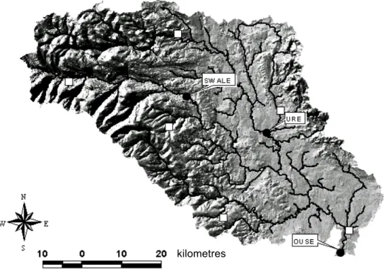
The River Ouse, situated in northern England and draining to the east into the Humber estuary, is formed by the confluence of the rivers Swale and Ure, and is later joined by the River Nidd (Fig. 1). At the catchment outlet, at Skelton, the river Ouse drains a total area of about 3500 km2. The catchment is dominated by Carboniferous Limestone and Millstone Grit in the Pennine hills in the west, and by Permian and Triassic rocks in the east (Jarvie et al., 1997b). The elevation varies from 714 m at the highest point in the catchment to 2.5 m at the outlet. The digital elevation model (DEM) and the river network are illustrated in Fig. 1. The climate is maritime with mild winters and warm summers. The mean annual precipitation is around 870 mm, evenly distributed throughout the year. The average annual potential evapotranspiration is about 530 mm, with a gradient from 560 mm per year in the upper part of the catchment to 500 mm close to the outlet.
The River Ure drains an area of 980 km2 with the highest point being at 716 m and the lowest at 20 m above sea level. The topography is characterised by steep sided valleys in
the upper part of the Ure and flattens at the confluence with the River Swale. There is a strong rainfall gradient from 2000 mm per year in the upper catchment to 600 mm in the lower part. The geology is characterised mostly by Carboniferous Limestone and Carboniferous Millstone Grit. The River Swale drains an area of 1470 km2. Topography varies from 716 m to 20 m. The river originates in the Carboniferous rocks of the Pennines and flows eastwards through narrow steep sided glaciated valleys into the flat Vale of York. The annual rainfall, like for the Ure river, is characterised by a strong gradient varying from 1400 mm to 600 mm per year. The geology is dominated by Limestone. The River Nidd area is about 550 km2 with a rainfall gradient of between 1800 and 600 mm per year controlled by topography. The geology is characterised by Carboniferous Millstone Grit and Carboniferous Limestone.
Clay is the major soil present on the catchment (55% of the total area). Other soils present include clay loam (27%) and sandy loam (13%). The upper part of the basin is used for rough grazing while the lower and flatter part is cultivated mainly for cereal production (winter wheat). The catchment is mainly rural and the urban part is relatively small. As described by Law et al. (1997), the headwaters of many Pennine rivers are reservoired to ensure potable water supply. Additional details about human influence on the hydrology of the Ouse catchment can be found in Law et al. (1997) and Edwards et al. (1997).
Overall, water quality in the Ouse basin is good with
Fig. 1. River network and flow gauges (dark circles) and rainfall gauges (white squares) for the Ouse catchment.
reported mean flow-weighted concentrations for the 1993– 1996 period of 3.36 mg l-1 and 128.7 µg l-1, for nitrate and orthophosphorus, respectively (Neal and Robson, 2000). The nitrogen in the river system comes mainly from diffuse losses from agricultural areas (Jarvie et al., 1998). Most of the total nitrogen consists of nitrate with small proportions of nitrite and ammonium with the exception of the Nidd river (Jarvie et al., 1998). The positive relationship between the nitrate concentration and flow observed for the Swale and Nidd rivers indicates the dominance of diffuse losses from agricultural runoff (Jarvie et al., 1998). Soluble reactive phosphorus is related negatively to flow, indicating the importance of point sources in the total losses (Jarvie et al., 1998). This is confirmed by the strong correlation between boron concentration and soluble reactive phosphorus found by Neal et al. (1998a) for all the rivers, including the Ouse river, draining into the Humber estuary. Boorman and Shackle (2002) estimated the point source contribution to total losses of phosphorus and nitrogen to be 40 and 7%, respectively. Additional details about water quality in the Ouse catchment can be found in Jarvie et al. (1997a; 1998) and Neal et al. (1998a, b).
Modelling approach
The Soil and Water Assessment Tool, SWAT, (Arnold et al., 1999) is a time continuous and semi-spatially distributed model, developed to simulate the impact of management decisions on water, sediment and agricultural chemical yields in river basins in relation to soil, land use and management practices. The model represents the large-scale spatial variability of soil, land use and management practices by discretising the catchment into sub-units using a two step approach.
A topographic discretisation is done by dividing the catchment into sub-units based on a minimum drainage area. Then, each sub-catchment is divided into one or several homogeneous hydrological response units (HRUs) obtained by overlaying the soil and land use maps. The HRUs have no exact geographical location and no spatial link to each other; they are associated only to a sub-basin. The response of each HRU in terms of water, sediment, nutrient and pesticide transformations and losses are determined, then aggregated at the sub-basin level and routed to the catchment outlet through the channel network.
The hydrological model is based on the water balance equation in the soil profile where the processes simulated include precipitation, infiltration, surface runoff, evapotranspiration, lateral flow and percolation. Surface runoff volume is predicted from daily rainfall using the curve number equation (USDA-SCS, 1972). The value of the curve
number ranges from 30 to 100 and is determined by the hydrological soil group, cover type, management practices such as tillage, and hydrological conditions. In the original method, the curve number was selected based on three possible antecedent moisture conditions: dry (wilting point), average conditions, and wet (field capacity). This approach was improved by Williams and Laseur (1976) by allowing the curve number to vary continuously with soil moisture. On a daily basis, the curve number is expressed as a function of the minimum curve number (for dry conditions) and a correction factor that is based on the actual water content available in the whole soil profile. The curve number varies continuously between the curve number corresponding to dry conditions when the soil is at wilting point, and the curve number corresponding to wet conditions when the soil is fully saturated. The water that does not run off infiltrates into the soil. Percolation occurs when field capacity of a soil layer is exceeded and is determined based on a storage routing technique. The percolation rate is controlled by the hydraulic conductivity of the soil layer. SWAT partitions groundwater into two aquifer systems: a shallow unconfined aquifer which contributes to the return flow and a deep and confined aquifer that can be used for pumping purposes and which receives water draining from the shallow aquifer.
Flow routing is based on the principle of mass conservation and runs on a daily basis without iteration. Outflow for a specific reach is linked to inflow and to actual water storage in the reach through a storage coefficient. This coefficient, based on the travel time within the reach, is a function of flow rate and is determined using Manning’s equation. Routing characteristics including reach length, channel slope and depth, channel top width and side slope (channels are assumed to have a rectangular shape) are estimated from the digital elevation model.
mineralisation, immobilisation and plant uptake for P. The component of N mineralisation is adapted from the PAPRAN model (Seligman and Van Keulen, 1981), and considers two different organic pools: fresh organic N pool, associated with crop residue and microbial biomass, and the stable organic N pool, associated with the soil humus. Mineralisation from the fresh organic N pool is controlled by the carbon-nitrogen and carbon-phosphorus ratios. Organic N associated with humus is divided into active and stable pools, which are in equilibrium. Only the active pool of organic N is subjected to mineralisation. Similarly, the mineralisation of organic P associated with humus is estimated for each soil layer. Mineralisation of both phosphorus and nitrogen is adjusted according to soil moisture and temperature conditions. External sources of nutrients accounted for by SWAT include the addition of organic and/or inorganic fertilisers, and atmospheric deposition for nitrogen. Additional details about the N and P cycle simulated by SWAT can be found in Arnold et al. (1999). Plant uptake of nitrogen and phosphorus is one of the main loss pathways and is estimated using a supply and demand approach. The nutrient demand is computed on a daily basis, based on the optimal N and P crop concentration for each growth stage.
Particulate N and P removed with sediments are directly proportional to the sediment yield, to the concentration of nutrient in the top layer and an enrichment ratio based on the peak runoff and peak rainfall excess rate. The loss of phosphorus dissolved in surface runoff is based on the concept of partitioning pesticides into the solution and sediment phases as described by Knisel (1980). Losses of nitrate in surface runoff and percolation are determined from the nitrate concentration in the soil layers.
Model setup
MODEL PARAMETERISATION
A 50 × 50m raster digital elevation map was available. Gridded soil type (Boorman et al., 1995) and the ITE land cover (Fuller, 1993) were available. The elevation data were processed using the SWAT-ArcView interface, subdividing the catchment into 25 sub-basins. The DEM was used to estimate all routing characteristics that were kept unchanged for the remainder of the study. The dominant soil and land-use were determined resulting in one HRU, i.e. one unique soil type and land use combination per basin. Each sub-basin was assigned a runoff curve number based on the hydrological soil group, cover type and management practices as described previously. Six rainfall stations provided daily rainfall measurements for the 1986–1990 period. Daily measurements of maximum/minimum and
average air temperature were available for one station. The actual management practices included fertiliser applications in February, March and in April; the average fertiliser application rate is around 105 kg ha–1 for nitrogen and 19 kg ha–1 of phosphorus. The variables used during the calibration-validation exercise included daily water flow, suspended sediment, nitrate and ortho-phosphorus concentrations (measured on a weekly basis) covering the 1986–1990 period and were provided by the Environment Agency of England and Wales, the Land Ocean Interaction Study (Tindall and Moore, 1997), and the UK Ministry for Agriculture Fisheries and Food.
MODEL CALIBRATION
The software HYSEP (USGS, 1996) was used to separate measured flow for each gauging station into surface runoff and base-flow. The calibration consisted in modifying the curve number to minimise the difference between measured (estimated with HYSEP) and predicted surface runoff for the Ure, Swale and Ouse flow gauges (Fig.1) for the year 1986. The parameters controlling the shallow aquifer balance were modified to minimise the difference between predicted and measured base-flow, while avoiding any long-term trend in groundwater storage. No adjustment was made for the nutrient transformation and transport. The accuracy of the model predictions were evaluated using the coefficient of efficiency (E) defined as follows:
(
)
(
)
∑
∑
= =
− − −
= n
i
obs obs n
i
obs mod
I I
I I E
i i i
1
2 1
2
1 (1)
where n represents the number of observations in the time series, Iobs is the observed value of the variable, Imod is the predicted value of the variable, and Iobs represents the mean measured value of the variable.
RESULTS
at Crakehill outlets, respectively. The major source of error in the prediction is linked to the spatial distribution of rainfall: SWAT being a semi-distributed model (sub-basins are the smallest units with geographic location), only one rainfall station can be associated to one sub-basin. This can alter flow prediction for areas that are characterised by a rainfall gradient, such as for the Swale sub-basin where the rainfall varies between 1400 and 600 mm yr–1. The overall simulation could have been improved by discretising the catchment into a larger number of sub-basins. However, it was preferred to discretise the catchment so that each sub-basin outlet corresponds to an actual gauging flow station. The coefficient of efficiency is higher for the general outlet
because the errors due to the rainfall spatial distribution balance out for the whole catchment. The model reproduced the peak runoff accurately but tended to over-predict the low flows during the summer months for the whole catchment (Table 1). The problem with the low flow prediction might be linked to the over-simplified groundwater component of SWAT. As explained earlier, for each sub-basin, the base-flow originates from the shallow aquifer. This is represented as a reservoir recharged by deep percolation and transmission losses, which empties into the river based on a recession coefficient independent of the gradient existing between the water table and the water level
0 50 100 150 200 250 300 350 400 450 500
0 50 100 150 200 250 300 350 400 450 500
1:1
0 50 100 150 200 250 300 350 400 450 500
Jan-86 Jan-87 Jan-88 Jan-89 Jan-90
predicted flow measured flow
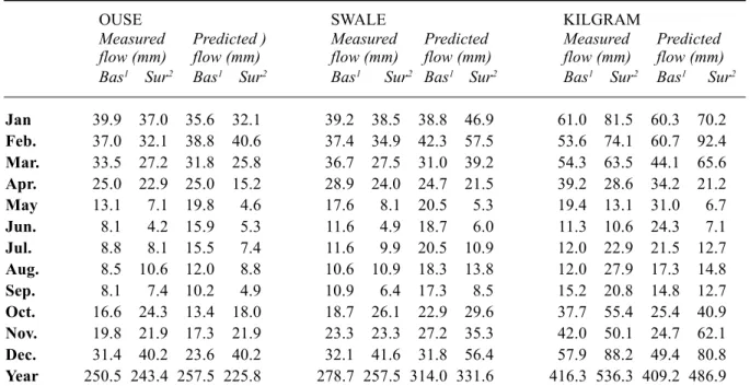
Table 1. Predicted and measured surface runoff and base-flow for the Ouse, Kilgram Bridge (Ure), and the Swale at Crakehill outlets
OUSE SWALE KILGRAM
Measured Predicted ) Measured Predicted Measured Predicted
flow (mm) flow (mm) flow (mm) flow (mm) flow (mm) flow (mm)
Bas1 Sur2 Bas1 Sur2 Bas1 Sur2 Bas1 Sur2 Bas1 Sur2 Bas1 Sur2
Jan 39.9 37.0 35.6 32.1 39.2 38.5 38.8 46.9 61.0 81.5 60.3 70.2
Feb. 37.0 32.1 38.8 40.6 37.4 34.9 42.3 57.5 53.6 74.1 60.7 92.4
Mar. 33.5 27.2 31.8 25.8 36.7 27.5 31.0 39.2 54.3 63.5 44.1 65.6
Apr. 25.0 22.9 25.0 15.2 28.9 24.0 24.7 21.5 39.2 28.6 34.2 21.2
May 13.1 7.1 19.8 4.6 17.6 8.1 20.5 5.3 19.4 13.1 31.0 6.7
Jun. 8.1 4.2 15.9 5.3 11.6 4.9 18.7 6.0 11.3 10.6 24.3 7.1
Jul. 8.8 8.1 15.5 7.4 11.6 9.9 20.5 10.9 12.0 22.9 21.5 12.7
Aug. 8.5 10.6 12.0 8.8 10.6 10.9 18.3 13.8 12.0 27.9 17.3 14.8
Sep. 8.1 7.4 10.2 4.9 10.9 6.4 17.3 8.5 15.2 20.8 14.8 12.7
Oct. 16.6 24.3 13.4 18.0 18.7 26.1 22.9 29.6 37.7 55.4 25.4 40.9
Nov. 19.8 21.9 17.3 21.9 23.3 23.3 27.2 35.3 42.0 50.1 24.7 62.1
Dec. 31.4 40.2 23.6 40.2 32.1 41.6 31.8 56.4 57.9 88.2 49.4 80.8
Year 250.5 243.4 257.5 225.8 278.7 257.5 314.0 331.6 416.3 536.3 409.2 486.9
1 Bas=base-flow estimated by Hysep, 2 Sur=surface runoff estimated by Hysep Fig. 2. Measured and predicted daily flow at the Ouse catchment
outlet.
Fig. 3. Measured v. predicted daily flow at the Ouse catchment outlet.
Measured flow (m3 s–1)
Predicted flow
(m
3 s –1)
Flow
(m
in the river. Using this type of approach, it will be very difficult to predict correctly long-lasting constant base-flow such as that occurring in summer 1989 (Fig. 2). The coefficient of efficiency for daily flow predictions for the Ouse general outlet is very similar to that obtained by Kuchment et al. (1996) that used a fully distributed, physically-based finite element model to predict water flow during the 1986–1990 period. Kuchment et al. (1996) obtained a coefficient of efficiency of 0.82; while using SWAT the coefficient of efficiency was 0.77.
The model estimates the monthly nitrate losses at the general outlet satisfactorily (Fig. 4); the coefficient of efficiency for the nitrate load predictions on a monthly basis is 0.64. The performance of the model could have been improved by using a more detailed description of the management practice for the whole basin. However, due to the lack of information, one unique yearly management plan was used for each land use. A similar conclusion was reached by Lewis et al. (1997) who applied the QUASAR model to simulate water quality in the Yorkshire Ouse. Their predictions for both water flow and water quality determinands compared reasonably well with the measured values, however, it was shown that the quality of the predictions is highly dependent upon the quality of the
inputs. The model captured well the seasonality of the nitrate losses. The highest losses occur from November until April, and the lowest losses during the May-October period (Fig. 5). The model also captured the impact of the fertilisation on the nitrate load occurring in April. The overestimation of nitrate losses during the summer months is explained by the overestimation of the flow during that period. The model performances for monthly ortho-phosphorus load predictions were not as good due to the simplified scheme for nutrient input (E=0.02). The predicted and measured seasonal losses of ortho-phosphorus are shown in Fig. 6. The underprediction during the summer months is probably linked to the input coming from point sources. Overall, the model performances are acceptable and the data used for the validation are quite representative of the catchment conditions. The measured and predicted flow weighted concentrations for the 1986–1990 period are 3.51 mg l–1 and 3.38 mg l–1, and 174 µg l–1 and 140.7 µg l–1, for nitrate and ortho-phosphorus, respectively. These concentrations are similar to those reported by Neal and Robson (2000) for the 1993–1996 period with a mean flow weighted concentrations of 3.36 mg l–1 and 127.7 µg l–1, for nitrate and ortho-phosphorus, respectively.
The model captured the importance of annual rainfall on the annual nitrate losses at the catchment outlet. The correlation coefficients between the annual nitrate load and the annual rainfall are 0.93 and 0.61 for the measured and predicted series, respectively. Even though these values differed because of errors in both the flow and nitrate load predictions, these significantly high coefficients of correlation indicate that the model captured well the observed impact of rainfall on the annual losses of nitrate. The model proved to be responsive to both management practices and climate. It was thus assumed that SWAT could be used to study the impact of climate change on nutrient loads in the Ouse catchment.
0.0E+00 5.0E+05 1.0E+06 1.5E+06 2.0E+06 2.5E+06
Jan-86 Jan-87 Jan-88 Jan-89 Jan-90
N
O
3 l
o
ad (
k
g)
measured load predicted load
Fig. 4. Measured and predicted monthly nitrate losses.
0.E+00 1.E+05 2.E+05 3.E+05 4.E+05 5.E+05 6.E+05 7.E+05 8.E+05 9.E+05 1.E+06
jan feb mar apr may jun jul aug sep oct nov dec
NO3 load (kg)
measured load predicted load fertiliser application
0.0E+00 5.0E+03 1.0E+04 1.5E+04 2.0E+04 2.5E+04 3.0E+04 3.5E+04 4.0E+04
jan feb mar apr may jun jul aug sep oct nov dec
O
rth
o
P
l
o
a
d
(k
g
)
measured load predicted load
Fig. 5. Measured and predicted seasonal nitrate losses during 1986-1990 period.
Uncertainty analysis
To assess the significance of the potential changes introduced by the climate scenarios, an uncertainty analysis was conducted. The following variables were then chosen to assess the uncertainty associated with the selection of the calibrated set of variables:
z curve number: variable used to determine the partition of rainfall into surface runoff and infiltration;
z saturated hydraulic conductivity: variable used to compute the water redistribution in the soil profile; z available water capacity: variable defined as the
difference between the field capacity and wilting point; z recession coefficient: variable used in the estimation of
the groundwater contribution to the base-flow; z groundwater-root zone coefficient: variable that controls
the amount of water that can contribute to the unsaturated zone to allow plant transpiration from the shallow aquifer.
Based on these variables, 1000 Monte-Carlo simulations were made. The variables were drawn independently from a uniform distribution allowing a variation of ±30%. Since the curve number on certain areas of the catchment was around 89, the variation of the curve number was restricted to ±10% to avoid exceeding the maximum possible curve number value (maximum curve number is 100 and corresponds to impervious areas). Each realisation comprised a fifteen years’ run. The results for the statistical distribution of the annual runoff are shown in Fig. 7. The simulated water yield ranged from 223 to 375 mm year–1. Using the Lilliefors (1967) test, the data could be approximated, at the 0.05 significance level, by a lognormal
distribution. The parameters of the three-parameter lognormal distribution are 223 mm (shift), and 3.743 (mean) and 0.458 (variance) for the log of the data. The minimum variance unbiased estimator of the mean of the lognormal distribution was computed as described by Gilbert (1987) as 276.1 mm yr–1. The estimated standard deviation is 40.5, and the upper and lower 95% confidence intervals for the mean were calculated to be 278.2 and 274.2 mm yr–1. The procedure for computing the median and its confidence interval is given by Gilbert (1987) and the results were 264.6, 262.7, and 267 mm yr–1, respectively. The runoff for the 15 years baseline simulation (262.93 mm yr–1) falls within the 95% confidence interval of the median, but outside the 95% confidence interval for the mean. However, the results show the robustness of the model. Even when large perturbations were introduced for the hydrological parameters (by 60% for all parameters but 20% for the curve number) the difference between the mean and the median runoff of the 1000 realisations is less than 5% of the predicted runoff for the baseline simulation.
Climate scenarios
The study followed the impact approach described by Carter et al. (1994) using a three stage approach: calibrate and validate the model using climatic measurements; define the climate change scenarios and perturbation to be applied to the actual climate data; and run the model using the baseline and perturbed climate time series. Climate scenarios were developed from the output of climatic GCM experiments and consist of a monthly-based variation of the precipitation and temperature. The climate stations (six gauges for rainfall and one for temperature) included in the validation study were used to represent the actual climate of the whole catchment. The 30-year measured time series of daily rainfall and temperature covering the 1961–1990 period is referred to as the baseline climate. This period, as noted by Marsh and Sanderson (1997), includes both unusual rainfall patterns with an increase in the ratio between winter and summer precipitation and acute drought years such as 1989 and 1990. Furthermore, temperatures observed since 1976 have increased by 0.4°C (Marsh and Sanderson, 1997). These characteristics were also observed during the LOIS study period of 1993–1996 (Marsh and Sanderson, 1997), indicating a persistence in the changes, both in terms of temperature increase and in the occurrence of extreme hydrological events.
Four GCMs reviewed thoroughly by the Inter-governmental Panel on Climate Change (IPCC, 1996) were used: CSIRO-Mk2 (Hirst et al., 1996), ECHAM4 (Roeckner et al., 1996), CGCM1 (Flato et al., 1999), and HadCM2 3 Parameter Lognormal Distribution
Annual Runoff (mm)
No of obs
0 20 40 60 80 100 120 140 160 180 200 220 240
0 42 85 127 170
Fig. 7. Distribution of the annual runoff computed from the Monte-Carlo simulation of 1000 runs along with the fitted lognormal
(Johns et al., 1997). Four transient scenarios of 30 years centred on the year 2050 were selected for each of the GCMs, as well as for HadCM2, two additional scenarios centred on the years 2020 and 2080. For each of the climate scenarios, two variables were used: precipitation and temperature. The climate change variables are given in percentage change for precipitation (multiplicative variable) and degrees Celsius change for temperature (additive variable), and the changes are summarised in Table 2. The perturbations of the baseline daily times series were carried out simply by adding the estimated change in temperature (oC) in each month to the baseline temperature of every day of that month. Similarly, the baseline daily precipitation of each month was multiplied by the estimated change in precipitation (%) in that month to obtain the daily perturbation.
The cluster of scenarios for 2050 suggests an increase between 2.0–2.9oC for the mean annual temperature and an increase of the annual precipitation. For Echam2050, a 4.9% reduction of precipitation is predicted, more pronounced during the summer (more than 25% decrease). The other cluster of climate change scenarios predicts an increase in the annual precipitation from 8.43% (HadCM2 2020) to 18.13 % (HadCM2 2080).
Impact of climate change on nutrient
loads from agricultural areas
The calibrated and validated setup comprising 25 sub-basins was used with the present 30 years climate to generate the
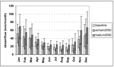
baseline scenario. The results will concentrate on the two scenarios that showed the most extreme behaviours, i.e. Echam2050 and HadCM2050. The HadCM2050 scenario predicts an increase of stream-flow by more than 120 mm yr–1 while Echam2050 predicts a decrease by about 70 mm yr–1. The increase in rainfall for the HadCM2050 scenario also resulted in an increase in the proportion of water lost through surface runoff. These extreme behaviours are explained fully by the difference in the projection of rainfall between the two scenarios. For the HadCM2050 scenario, the water flow predicted is always higher than that of the baseline, while for Echam2050 it is always lower except for the month of December (Fig. 8). Both climate scenarios predict an increase in the actual evapotranspiration. The increase is higher for the HadCM2050 because water is not limited due to the high precipitation while, for the Echam2050 climate scenario, the decrease in rainfall in summer limits the amount of water that can be lost through evapotranspiration (Fig. 9). A two-tailed paired t-test was conducted, and the differences between the baseline and the two scenarios for both stream-flow and actual evapotranspiration were statistically significant (0.10 significance level) for all months.
Concerning nitrate and ortho-phosphorus uptake, both scenarios show a similar trend with the highest consumption taking place from May to September. However, both climate change scenarios introduced an early shift in the plant growth resulting in higher uptake from May to June and a lower uptake in August as compared to the baseline. This early shift is due to the higher temperature which induced an earlier growth, as illustrated by the higher actual Table 2. Change of precipitation (%) and temperature (°C) as predicted by the different climate scenarios
.
HADCM 2020 HADCM 2050 CGCM1 2050 CSIRO 2050 ECHAM 2050 HADCM 2080
P (%) T (°C) P (%) T (°C) P (%) T (°C) P (%) T (°C) P (%) T (°C) P (%) T (°C)
Jan 16 1.1 14 2.0 23 1.9 –4 1.4 –4 3.4 4 2.6
Feb. 21 2.3 24 2.9 21 1.3 6 2.0 0 3.1 24 3.2
Mar. 7 1.7 7 2.4 21 1.2 19 2.2 5 2.8 10 2.5
Apr. –2 0.8 9 2.0 10 1.6 10 2.1 –8 2.8 18 2.7
May –10 0.8 5 1.8 –1 1.5 5 2.2 –1 2.4 31 2.8
Jun. 0 1.2 4 1.7 2 2.0 –1 1.8 –21 2.7 –6 2.2
Jul. 20 0.9 9 1.8 5 2.3 18 2.0 –24 3.7 –14 2.7
Aug. –1 1.1 1 1.9 12 2.6 4 1.9 –25 3.7 19 2.4
Sep. –2 1.6 15 1.6 15 2.7 7 1.7 –13 2.8 21 2.7
Oct. 18 1.2 22 1.9 –7 2.3 11 2.1 –1 2.4 38 2.9
Nov. 26 1.4 43 2.6 3 2.9 12 2.6 3 2.7 43 3.8
Dec. 2 0.6 14 1.8 11 2.2 9 2.6 18 2.8 18 3.1
evapotranspiration. The decrease in August can be explained by the effect of limited available nutrient in the soil profile due to higher uptake during the previous months, because of faster crop growth. The Echam2050 scenario predicts an increase of 26 and 30% for nitrate and ortho-phosphorus uptake, respectively. These changes are limited to 21 and 17% for the HadCM2050 scenario. The differences might be explained by the higher increase in temperature projected by the Echam2050 scenario, accelerating the organic matter mineralisation processes.
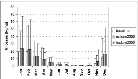
The impact of climate change on nutrient loads was analysed in terms of total nitrogen obtained as the sum of nitrate and particulate organic nitrogen losses, and total phosphorus obtained as the sum of ortho-phosphorus and
particulate phosphorus losses. Both climate scenarios show an increase in total nitrogen losses in winter-period, and a slight or no change in spring and summer (Fig. 10). On an annual basis both scenarios predict an increase in total phosphorus losses, however with strong seasonal differences. The Echam2050 scenario shows a strong decrease of total phosphorus losses during the summer due to the flow and sediment decrease (Fig. 11). Furthermore, the earlier plant growth also reduces erosion from agricultural fields. Both scenarios show an increase in total phosphorus losses in winter independently of the trend of the flow, illustrating probably an enrichment of the topsoil in phosphorus. The results were also analysed statistically using a two-tailed paired t-test. The difference for total
0 20 40 60 80 100 120
Jan Fe
b
Ma
r
Ap
r
Ma
y
Ju
n
Ju
l
Au
g
Se
p
Oc
t
No
v
De
c
st
ream
fl
o
w
(m
m
/m
o
n
th
)
baseline
echam2050
hadcm2050
0 20 40 60 80 100 120 140
Jan Fe
b
Ma
r
Ap
r
Ma
y
Ju
n
Ju
l
Au
g
Se
p
Oc
t
No
v
De
c
A
E
T (
m
m
/m
o
nt
h)
baseline
echam2050
hadcm2050
Fig. 8. Mean monthly stream-flow for the baseline and the climate changes scenarios (±1 standard deviation).
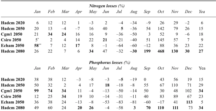
phosphorus losses was statistically significant for Echam2050 for all months except for May, and for total nitrogen only December and August showed a significant difference. Concerning HadCM2050, only the months of January, May and August showed significant difference for total nitrogen, and all the months but March, April and August for total phosphorus. For all the other months, the seasonal variability of the baseline simulation hid the impact of the climate change. On an annual basis, the changes introduced by both climate changes are significant for stream-flow, actual evapotranspiration, total nitrogen and phosphorus losses. This is confirmed for all scenarios (Table 3). The nitrogen loss changes, as predicted by all climate scenarios, ranged from 6 to 27%, and from 5 to 34% for
phosphorus. It is important to note that all scenarios do not always agree on a seasonal basis on the magnitude and the direction of change for nutrient losses, but they all agree in predicting the increase in annual nutrient losses (Table 3).
Then, as discussed by Hanratty and Stefan (1998), a precision analysis compared the root mean square error between the predicted and measured water quantity and nutrient loads with the root mean square difference between the baseline and the simulated climate change scenarios. The root mean square differences for water flow, total phosphorus and nitrogen losses were higher than the root mean square errors, indicating that the changes induced by the different scenarios were measurable (Haratty and Stefan, 1998). Similar results were obtained for the other four
0.00 0.05 0.10 0.15 0.20 0.25 0.30 0.35 0.40
Jan Fe
b
Ma
r
Ap
r
Ma
y
Ju
n
Ju
l
Au
g
Se
p
Oc
t
No
v
De
c
P
l
o
sses
(
k
g
/h
a
)
baseline echam2050
hadcm2050 0
10 20 30 40 50 60 70 80
Jan Feb Mar Apr May Jun Jul Aug Sep Oct Nov Dec
N losses (kg/ha)
baseline echam2050
hadcm2050
Fig. 10. Mean monthly nitrogen losses for the baseline and the climate changes scenarios (±1 standard deviation).
Table 3. Change of total nitrogen (N) and total phosphorus (P) losses (%) as predicted by the different climate scenarios.
Nitrogen losses (%)
Jan Feb Mar Apr May Jun Jul Aug Sep Oct Nov Dec Yea
Hadcm 2020 6 12 12 1 –3 2 –4 –34 –9 26 29 –2 6
Hadcm 2050 20 13 –4 –7 16 40 5 –36 54 142 79 26 15
Cgm1 2050 21 34 24 16 16 9 –36 –50 3 52 9 –6 18
Csiro 2050 5* 2 4 14 22 21 –21 –40 51 145 57 7 9
Echam 2050 58** 7 12 17 8 –1 –64 –60 –12 88 36 23 22
Hadcm 2080 26 22 7 6 34 47 –32 –30 199 468 130 30 27
Phosphorus losses (%)
Jan Feb Mar Apr May Jun Jul Aug Sep Oct Nov Dec Yea
Hadcm 2020 38 38 12 –3 –8 –3 –5 –19 0 43 56 19 15
Hadcm 2050 50 32 2 4 17 18 –18 –8 55 67 110 71 29
Cgm1 2050 99 74 34 11 –4 –13 –50 –14 50 30 48 102 34
Csiro 2050 12 25 34 19 10 –14 –31 –11 40 83 89 67 23
Echam 2050 36 38 24 –13 –8 –53 –83 –81 –60 –17 41 113 5
Hadcm 2080 49 60 24 20 26 –4 –58 3 70 110 111 73 34
*for each month, the minimum predicted change of all scenarios is underlined, ** for each month, the maximum predicted change of all scenarios is
underlined and written in bold characters
climate change scenario runs. The significance of the impacts of climate change on stream-flow is also confirmed by the results of the sensitivity analysis, the predicted changes in annual water flow being greater than 5%.
Conclusions
The SWAT model was applied to a UK catchment to assess the impact of potential climate change on nutrient loads to surface water. The study was conducted using a three-step procedure: validate the hydro-geochemical model using measured climate data, perturb the baseline climate data according to the different climate scenarios, and then run the model using the modified baseline climate. All climate scenarios except Echam2050 predict an increase in surface water flow. This increase is statistically significant and the changes are higher than the errors made in the calibration exercise. All six climate scenarios would affect, significantly, not only water quality and nutrient loads from agricultural areas but also crop growth patterns. This agrees with other studies (Kallio et al., 1997; Haratty and Stefan, 1998). One of the major conclusions is that climate changes, as actually predicted, will increase the nutrient losses to surface water firstly by accelerating soil processes such as mineralisation of organic matter and, for all climate scenarios except
Echam2050, by increasing the amount of water transiting through the soil profile to the river network. Furthermore, all scenarios predict a shift in crop growth. This will affect soil and crop management, so that traditional crop rotations and management practices will have to be adjusted.
Acknowledgements
This work was carried out within the framework of the CHESS project (Climate and Hydrochemistry and Economics of Surface Water Systems), financed by the European Commission under contract ENV4-CT97-0440. The authors wish to thank David Boorman and Victoria Shackle (Centre for Ecology and Hydrology, Wallingford) for providing the data used during this project.
References
Allen, M.R., Stott, P.A., Mitchell, J.F.B., Schnur, R. and Delworth, T.L., 2000. Quantifying the uncertainty in forecasts of anthropogenic climate change. Nature, 407, 617–620. Arnell, W., 1999. The effect of climate change on hydrological
Arnold, J.G., Williams, J.R. and Srinivasan, R., 1999. SWAT98.1 Manual, USDA, Agricultural Research Service and Blackland Research Center, Texas A&M University, U.S.A.
Beniston, M. and Tol, R.S.J., 1998. Europe. In: The regional impact of climate change: An assessment of vulnerability, Special Report of IPCC Working Group II, R.T. Watson, M.C. Zinoywera, R.H. Moss and D.J. Dokken (Eds.), Cambridge University Press, Cambridge, UK, 149–185.
Boorman, D.B. and Shackle, V.J., 2002. CHESS: climate, hydrochemistry and economics of surface water systems final report. CEH, Wallingford, 112 pp.
Boorman, D.B., Hollis, J.M. and Lilly, A., 1995. Hydrology of soil types: a hydrological based classification of the soils of the United Kingdom. Institute of Hydrology, Report 126, Wallingford, UK.
Carter, T.R., Parry, M.L., Nishioka, S. and Harasawa, H., 1994. Technical guidelines for assessing climate change impacts and adaptations. IPCC Working Group II. University College London and Center for Global Environmental Research, Japan. 60 pp.
Edwards, A.M.C., Freestone, R.J. and Crockett, C.P., 1997. River management in the Humber catchment. Sci. Total. Envir., 194/ 195, 235–246.
Flato, G.M., Boer, G.J., Lee, W.G., McFarlane, N.A., Ramsden, D., Reader, M.C. and Weaver, A.J., 1999. The Canadian centre for climate modelling and analysis global coupled model and its climate. Climate Dynamics, 16, 451–467.
Fuller, R.M., 1993. The land-cover map of Great Britain. Earth Space Rev., 2, 13–18.
Gilbert, O.R., 1987. Statistical methods for environmental pollution monitoring. VanNostrand Reinhold, New York, 320 pp.
Gleick, P.H., 1999. Studies from the water sector of the national assessment. J. Amer. Water. Resour. Assoc., 35, 1429–1442. Hanatty, M.P. and Stefan, H.G., 1998. Simulating climate change
effects in a Minnesota Agricultural watershed. J. Environ. Qual.,
27, 1524–1532.
Hirst, A.C., Gordon, H.B. and O’Farrell, S.P., 1996. Global warming in a coupled climate model including oceanic eddy-induced advection. Geophys. Res. Lett., 23, 3361–3364. Hulme, M. and Carter, T.R., 1999. Creating climate scenarios for
the European ACACIA assessment. In: Climate Scenarios for Agricultural, Forest, and Ecosystems Impact, ECLAT-2 Report No 2, Potsdam Workshop Proceedings.
IPCC, 1996. Climate change 1995: the science of climate change J.T. Houghton, L.G. Meiro Filho, B.A. Callendar, N. Harris, A. Kattenberg and K. Maskell (Eds.), Cambridge University Press, Cambridge, UK. 572 pp.
IPCC, 2001. IPCC third assessment report, summary for policymakers. Contribution of WGII, Climate Change 2001: Impacts, Adaptation and Vulnerability.
Jarvie, H.P., Neal, C., Leach, D.V., Ryland, G.P., House, W.A. and Robson, A.J., 1997a. Major ion concentrations and the inorganic carbon chemistry of the Humber rivers. Sci. Total. Envir., 194/195, 285-302.
Jarvie, H.P., Neal, C. and Robson, A.J., 1997b. The geography of the Humber catchment. Sci. Total. Envir., 194/195, 87-99. Jarvie, H.P., Whitton, B.A. and Neal, C., 1998. Nitrogen and
phosphorus in east coast Bristish rivers: speciation, sources and biological significance. Sci. Total. Envir., 210/211, 79–109. Johns, T.C., Carnell, R.E., Crossley, J.F., Gregory, J.M., Mitchell,
J.F.B., Senior, C.A., Tett, S.F.B. and Wood, R.A., 1997. The second Hadley Centre coupled ocean-atmosphere GCM: Model description, spinup and validation. Climate Dynamics, 13, 103– 134.
Kallio, K., Rekolainen, S., Ekholm, P., Granlund, K., Laine, Y., Johnsson, H. and Hoffman, M., 1997. Impacts of climatic change on agricultural nutrient losses in Finland. BorealEnviron. Res.,
2, 33–52.
Knisel, W.G., 1980. CREAMS, A field scale model for chemicals, runoff and erosion from agricultural management systems, U.S. Dept. Agric. Conserv. Res. Rept. No. 26.
Kuchment, L.S., Demidiv, V.N., Naden, P.S., Cooper, D.M. and Broadhurst, P., 1996. Rainfall-runoff modelling of the Ouse basin, North Yorkshire: an application of a physically based distributed model. J. Hydrol., 181, 323–342.
Law, M., Wass, P. and Grimshaw, D., 1997. The hydrology of the Humber catchment. Sci. Total. Envir..,194/195, 119–128. Lewis, D.R., Williams, R.J. and Whitehead, P.G., 1997. Quality
simulation along river systems (QUASAR). An application to the Yorkshire Ouse. Sci. Total. Envir.., 194/195, 399-418. Lilliefors, H.W., 1967. On the Kolmogorov-Smirnov test for
normality with mean and variance unknown. J. Amer. Stat. Assoc., 64, 399–402.
Marsh, T.J. and Sanderson, F.J., 1997. A review of hydrological conditions throughout the period of the LOIS monitoring programme: considered within the context of the recent UK climatic volatility. Sci. Total. Envir.,194/195, 59–69. Mitchell, T.D. and Hulme, M., 1999. Predicting regional climate
change: living with uncertainty. Prog. Phys. Geog., 23, 57–78. Murdoch, P.S., Baron, J.S. and Miller, T.L., 2000. Potential effects of climate change on surface-water quality in North America. J. Amer. Water Resour. Assoc., 36, 347–366.
Neal, C. and Robson, A.J., 2000. A summary of water quality data collected within the Land-Ocean Interaction Study: core data for the eastern UK rivers draining to the North Sea. Sci. Total. Envir.,251/252, 585–665.
Neal, C., Fox, K.K., Harrow, M.. and Neal, M., 1998a. Boron in the major UK rivers entering the North Sea. Sci. Total. Envir.,
210/211, 41–51.
Neal, C., House, W.A., Whitton, B.A. and Leeks, G.A., 1998b. Conclusions to special issue: water quality and biology of United Kingdom Rivers entering the North Sea: Land-Ocean Interaction Study (LOIS) and associated work. Sci. Total. Envir.,210/211, 585–594.
Nijssen, B., O’Donnell, G.M., Hamlet, A.F. and Lettenmaier, D.P., 2001. Hydrologic sensitivity of global rivers to climate change. Climatic Change, 50, 143–175.
Novotny, V. and Olem, H., 1994. Water quality, prevention, identification, and management of diffuse pollution. VanNostrand Reinhold, New York, 1954 pp.
Priestley, C.H.B. and Taylor, R.J., 1972. On the assessment of surface heat flux and evaporation using large scale parameters. Mon. Weather Rev., 100, 81–92.
Reilly, J., Stone, P.H., Forest, C.E., Webster, M.D., Jacoby, H.D. and Prinn, R.G., 2001. Uncertainty and climate change assessment. Science, 293: 430–431, 433.
Ritchie, J.T., 1972. A model for predicting evaporation from a row crop with incomplete cover. Water Resour. Res., 8, 1204– 1213.
Roeckner, E., Arpe, K., Bengtsson, L., Christoph, M., Claussen, M., Dümenil, L., Esch, M., Giorgetta, M., Schlese, U. and Schulzweida, U., 1996. The atmospheric general circulation model ECHAM-4: model description and simulation of present-day climate. Max-Planck Institute for Meteorology. Report No.218, Hamburg, Germany, 90 pp.
Tindall, C.I. and Moore, R.V., 1997. The Rivers Database and overall data management for the Land Ocean Interaction Study programme. Sci. Total. Envir., 194/195, 129-135.
U.S. Department of Agriculture, Soil Conservation Service, 1972. National Engineering Handbook, Hydrology Section 4, Chapters 4–10.
U.S. Geological Survey, 1996. A computer program for streamflow hydrograph separation and analysis. Water Investigation Report 96-4040.
Visser, H., Folkert, R.J.M., Hoekstra, J. and DeWolff, J.J., 2000. Identifying key sources of uncertainty in climate change projections. Climatic Change, 45, 421–457.
Williams, J.R., 1975. Sediment routing for Agricultural Watersheds. Water Res. Bull., 11, 965–974.