www.earth-syst-dynam.net/6/327/2015/ doi:10.5194/esd-6-327-2015
© Author(s) 2015. CC Attribution 3.0 License.
The ocean carbon sink – impacts, vulnerabilities and
challenges
C. Heinze1,2, S. Meyer1, N. Goris1,2, L. Anderson3, R. Steinfeldt4, N. Chang5, C. Le Quéré6, and D. C. E. Bakker7
1Geophysical Institute, University of Bergen and Bjerknes Centre for Climate Research, Bergen, Norway 2Uni Research Climate, Bergen, Norway
3Department of Marine Sciences, University of Gothenburg, Gothenburg, Sweden 4Institute of Environmental Physics, University of Bremen, Bremen, Germany
5Southern Ocean Carbon and Climate Observatory, Natural Resources and the Environment, CSIR,
Stellenbosch, South Africa
6Tyndall Centre for Climate Change Research, University of East Anglia, Norwich Research Park,
Norwich, UK
7Centre for Ocean and Atmospheric Sciences, School of Environmental Sciences, University of East Anglia,
Norwich Research Park, Norwich, UK
Correspondence to:C. Heinze ([email protected])
Received: 17 November 2014 – Published in Earth Syst. Dynam. Discuss.: 5 December 2014 Revised: 30 April 2015 – Accepted: 14 May 2015 – Published: 9 June 2015
Abstract. Carbon dioxide (CO2) is, next to water vapour, considered to be the most important natural
green-house gas on Earth. Rapidly rising atmospheric CO2 concentrations caused by human actions such as fossil
fuel burning, land-use change or cement production over the past 250 years have given cause for concern that changes in Earth’s climate system may progress at a much faster pace and larger extent than during the past 20 000 years. Investigating global carbon cycle pathways and finding suitable adaptation and mitigation strate-gies has, therefore, become of major concern in many research fields. The oceans have a key role in regulating atmospheric CO2concentrations and currently take up about 25 % of annual anthropogenic carbon emissions to
the atmosphere. Questions that yet need to be answered are what the carbon uptake kinetics of the oceans will be in the future and how the increase in oceanic carbon inventory will affect its ecosystems and their services. This requires comprehensive investigations, including high-quality ocean carbon measurements on different spatial and temporal scales, the management of data in sophisticated databases, the application of Earth system models to provide future projections for given emission scenarios as well as a global synthesis and outreach to policy makers. In this paper, the current understanding of the ocean as an important carbon sink is reviewed with re-spect to these topics. Emphasis is placed on the complex interplay of different physical, chemical and biological processes that yield both positive and negative air–sea flux values for natural and anthropogenic CO2as well as
on increased CO2(uptake) as the regulating force of the radiative warming of the atmosphere and the gradual
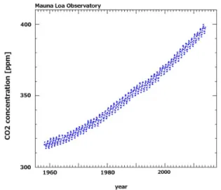
Figure 1. Atmospheric CO2 concentrations recorded at Mauna Loa Observatory between 1958 and 2014. Due to human-produced emissions, CO2levels in Earth’s atmosphere have been rapidly ris-ing since the beginnris-ing of the Industrial Revolution and nowadays are crossing 400 ppm (400.01 ppm on 25 May 2013), equalling a 44 % increase when compared to pre-industrial CO2 concentra-tions of around 278 ppm. Source: Dr Pieter Tans, NOAA/ESRL (http://www.esrl.noaa.gov/gmd/ccgg/trends) and Dr Ralph Keeling, Scripps Institution of Oceanography (http://scrippsco2.ucsd.edu/).
1 Historic background
In the atmosphere, carbon dioxide (CO2) occurs only in
a very small fraction (currently around 400 ppm; http:// scrippsco2.ucsd.edu/graphics_gallery/maunaloarecord.html; ppm=parts per million, ratio of the number of moles CO2in a given volume of dry air to the total number of moles of all constituents in this volume, see IPCC, 2013). Nevertheless, due to its high abundance as compared to other greenhouse gases, it is considered to be the overall most important green-house gas next to water vapour. Its importance in regulating the global heat budget was documented in the 19th century by Arrhenius (1886). Ultimately, the greenhouse effect of CO2can be linked to its molecule structure: vibrational and
rotational motions of the gaseous CO2 molecules resonate
with the thermal radiation leaving Earth’s surface at bands centred at different discrete wavelengths, thereby heating up the lower atmosphere (e.g. Barrett, 2005; Tomizuka, 2010). The main absorption band (combined vibrational and rotational resonance mode) of CO2is centred at 15 µm
wavelength (Wang et al., 1976; Liou, 1980). The incoming solar radiation is of short wavelength (mainly between 0.5– 1 µm). The thermal radiation outgoing from the Earth is of longer wavelength (typically between 5 and 20 µm). Without the natural greenhouse effect and under the assumption that solar absorption and albedo are kept fixed at the present-day values, an average temperature of −19◦C would dominate Earth’s surface instead of the actual average value of around 15◦C (Ramanathan et al., 1987).
The pre-industrial level of atmospheric CO2expressed as
a volume mixing ratio was around 278 ppm with minor fluc-tuations around this level (Siegenthaler et al., 2005) due to the natural variability of carbon reservoirs on land and in the ocean as well as volcanic activities and a small remaining trend going back to the last deglaciation (Menviel and Joos, 2012). The onset of the industrialization and the Anthro-pocene as the era of fundamental human impact on the Earth system (Crutzen, 2002) can be dated to around 1776 when the improved design of the steam engine by James Watt en-abled its operational use. The 300 ppm boundary was crossed in the early 20th century according to ice core measurements from Law Dome (Etheridge et al., 2001; samples from Law Dome core D08 show values of 296.9 and 300.7 ppm for mean air ages given in calendar years of 1910 and 1912 respectively, with an overall accuracy due to analytical er-rors and age determination erer-rors of±1.2 ppm). At the be-ginning of the instrumental record of atmospheric CO2 in
1958, its concentration was around 315 ppm (Keeling et al., 2001). Ten years ago (2003), we had arrived at 375 ppm. And now, we are crossing the 400 ppm level (400.01 ppm as of 25 May 2013; Fig. 1; Keeling et al., 2013). The largest con-tributor to this human-induced CO2release is firstly the
burn-ing of fossil fuel reserves, which normally would have been isolated from the atmosphere (Boden et al., 2011). Secondly, land-use change is a significant contributor followed by ce-ment production (Houghton, 1999; Boden et al., 2011). The warming effect due to the combustion of fossil fuel by human beings was first suggested and analysed by Callendar (1938). Since then, scientists have made attempts to quantify the fate of fossil fuels in conjunction with the natural carbon cycle. Bolin and Eriksson (1959) came up with a first estimate of the ultimate uptake capacity of the ocean for fossil fuel CO2
from the atmosphere: about 11/12 of CO2emissions would
ultimately accumulate in the ocean water column after re-peated oceanic mixing cycles and interaction with the cal-careous sediment, a process requiring several 10 000 years (see also Archer, 2005).
When it comes to the importance of human-produced greenhouse gases for changing the atmospheric heat budget and, hence, the climate system, CO2is by far the most
im-portant one. Other radiatively active trace gases like methane (CH4), halocarbons and nitrous oxide (N2O) have a higher
greenhouse potential per molecule than CO2, but are less
abundant in the atmosphere than CO2, so that CO2is the most
important anthropogenic driving agent of climate change (Myhre et al., 2013). The focus of this review is, thus, on CO2and the oceanic (“carbon”) sink. Future CO2emission
scenarios to drive climate models have been produced on empirical evidence concerning human behaviour and eco-nomics. In view of the on-going high-energy use in wealthy nations and the accelerating energy production in emerging economies (especially China and India; see Raupach et al., 2007), current and recent annual CO2 emission rates are at
pro-duced a few years ago for the climate projections of the Fifth Assessment Report of the IPCC (RCP scenarios; van Vuuren et al., 2011a, b; Peters et al., 2013). Considering the key role of the oceans in the global carbon budget it is there-fore fundamental to broaden our knowledge on their past, present and future quantitative impact in regulating atmo-spheric CO2concentrations.
2 General concepts of ocean carbon cycling
The oceans regulate atmospheric CO2mainly by two
mech-anisms: the first consists of the abiotic inorganic cycling of carbon that involves CO2 air–sea gas exchange (Liss
and Merlivat, 1986; Wanninnkhof, 1992; Nightingale et al., 2000), CO2dissolution (Weiss, 1974) and hydration to
car-bonic acid, dissociation of carcar-bonic acid (Dickson et al., 2007) as well as transport and mixing of total dissolved CO2
in seawater. The second mechanism describes the cycling of carbon due to biological activity.
2.1 Inorganic carbon cycle processes
Seawater is saline and contains practically all elements of the chemical periodic table. Due to its slightly alka-line behaviour, it can keep the ionic compounds of weak acids in solution. Carbon dioxide, or carbonic acid (H2CO3)
when combined with water (H2O), dissociates in
seawa-ter mostly into bicarbonate (HCO−
3) and carbonate (CO2−3 ),
while only a small amount of the CO2is kept in its dissolved
state (as an order of magnitude estimate the partitioning of HCO−
3 : CO2−3 : CO2is 100 : 10 : 1 but significant deviations
from this can occur especially with respect to CO2). The sum
of HCO−
3, CO2−3 and CO2is called “total dissolved inorganic
carbon” (DIC). A huge reservoir of DIC has been built up in the oceans over geologic time through the interaction of sea-water with sediments, weathering from land, gas exchange with the atmosphere, and outgassing from the Earth’s inte-rior. At pre-industrial times, this DIC pool is 65 times as large as the atmospheric pre-industrial CO2reservoir and
ap-proximately 20 times as large as the carbon on land bound to living and dead biomass including soils (Degens et al., 1984; Falkowski et al., 2000).
DIC is distributed in the oceans as passive tracer (like dye) by currents and turbulent mixing. In a simplistic model, transportation of carbon in the oceans mainly follows the large-scale ocean circulation: in the northern North Atlantic, surface waters are moved to the deep sea in a process of deep-water formation. The solubility of CO2gas in seawater
in-creases with decreasing temperature. As newly formed deep water is cold, the downward transport of the carbon frac-tion dissolved in seawater due to high CO2solubility is also
called the solubility pump (Volk and Hoffert, 1985). How-ever, the dissociation of CO2 into bicarbonate and
carbon-ate ions is antagonistic to the solubility and decreases with decreasing temperature and compensates to a certain degree
for this. In a theoretical ocean with only the solubility pump acting the overall surface to deep gradient of DIC would be slightly positive downwards. On its way through the ocean part of the deep water then upwells in the Southern Ocean around Antarctica, where it is blended with water masses from all oceans before it is re-cooled again to form deep and intermediate waters that spread into the Atlantic, Pacific, and Indian oceans. The circle is closed through the transport of upper water masses from the upwelling regions back to the deep-water production areas in the North Atlantic and the Southern Ocean (Broecker and Peng, 1982), which oc-curs via the Indian Ocean (“warm water path”) or via the Drake Passage (“cold water path” between South America and Antarctica; Rintoul, 1991). The water that has spent the longest time away from contact with the atmosphere is found in the northern Pacific Ocean below depths of about 2000 m and is approximately 1500 years old. Comparably, the hu-man perturbation of the carbon cycle has occurred only over the last 250 years, and diluting high anthropogenic carbon loads from the upper ocean with large deep-water reservoirs by mixing processes will take at least 6 times as long. Also, the slower oceanic circulation and mixing become with on-going climate change, the smaller the uptake rate of surface waters for human-produced carbon will be and the less effi-cient the ocean carbon sink will become for absorbing further CO2 additions to the atmosphere as carbonic acid
dissoci-ates less well into bicarbonate and carbonate in water of high pCO2.
2.2 Biological carbon pumps
While purely inorganic carbon cycling leads to a slight in-crease of DIC with depth, biological carbon cycling – via the two biological carbon pumps (Volk and Hoffert, 1985) – is responsible for most of the gradients existing in the real ocean DIC distribution. These gradients are mainly fu-elled by uptake of DIC by biota in the surface ocean to pro-duce particulate matter, the vertical flux of these particles, and degradation of these particles on their downward way through the water column. Biological carbon binding oc-curs mainly in the ocean surface layer, where phytoplank-ton through the process of photosynthesis produces biomass that can be utilized by other organisms on higher trophic levels (classical food chain). Next to dissolved CO2,
small particles do not sink anymore through the water col-umn but become suspended due to the increasing importance of friction for small particles, DOC is transported through the oceans like DIC as a passive tracer. While a large frac-tion of DOC may persist and accumulate in the water col-umn before being remineralized to inorganic substances, bi-ologically labile DOC is converted quickly (within minutes to days) in the upper ocean, predominantly by microbial ac-tivity (Carlson, 2002). By utilizing DOC, bacteria can build up exploitable biomass and part of the DOC may re-enter the classical food chain through the “microbial loop”. However, as the microbial loop itself includes several trophic levels, a large part of the recycled DOC is converted back to inor-ganically dissolved carbon along the process (Azam et al., 1983; Fenchel, 2008). In addition to microbial degradation, sorption onto larger particles, and UV radiation may consti-tute further important processes in the removal of dissolved organic matter (Carlson, 2002). The oceanic DOC pool is overall about 1 order of magnitude smaller than the marine DIC inventory but larger than the POC pool. Nevertheless, the highly reactive POC dominates the effect on variations in the oceanic DIC distribution. Most of the DOC is quite refractory which is consistent with its high radiocarbon age (4000–6000 years, Druffel et al., 1992). Thus, most of the marine DOC does not contribute much to the dynamics of carbon cycling in the ocean within the flushing timescale of the world ocean of about 1500 years. Next to POC and DOC cycling, the formation of calcium carbonate (CaCO3)
by shell- and skeleton-building marine organisms is of great importance in the ocean’s carbon cycle as it causes shifts in the overall DIC pool. HCO−
3 is converted to CO2−3 to produce
CaCO3. During this process, CO2is released to the
surround-ing water (Fig. 2, Eq. 3; Frankignoulle et al., 1994). Thus, the CaCO3pump is counteracting the organic carbon pump. As
more carbon is bound to POC and DOC during biological production than to CaCO3 (this rain ratio of CaCO3: POC
amounts globally averaged to about 15 % when counted in carbon atoms bound to particulate matter; Berelson et al., 2007), the CaCO3counter pump does nowhere fully
compen-sate for the organic carbon pump. Within the oceans, CaCO3
occurs either as aragonite or as calcite, with aragonite being more soluble at given conditions. The solubility of both com-pounds increases slightly at lower temperature and strongly with increasing depth (pressure) (Mucci, 1983; Zeebe and Wolf-Gladrow, 2001). Shell material sinking together with POC through the water column is usually degraded at larger depths than the organic material. Nevertheless, it is likely that also partial re-dissolution of calcitic and aragonitic plank-ton hard parts occurs in shallower depths than the respective CaCO3saturation horizon. Potential contributors to this are
e.g. zooplankton metabolisms (dissolution of shell material in copepod guts; Jansen and Wolf-Gladrow, 2001), local un-dersaturation hot spots due to lateral admixture of water or in micro-environments on biogenic particles due to remineral-ization of organic matter (Barrett et al., 2014), and admixture
Figure 2.Bjerrum plot created according to equations reviewed in Sarmiento and Gruber (2006) and Zeebe and Wolf-Gladrow (2001) as well as main reactions of carbon chemistry referred to in this review.
of larger amounts of Mg in the CaCO3 material (high-Mg
calcites; Feely et al., 2004).
The composition of the sinking material determines also its sinking velocity. Phytoplankton (plant plankton) and zoo-plankton (animal zoo-plankton) grazing on plant zoo-plankton or eat-ing other zooplankton can modify the vertical particle flux by producing a variety of carbonaceous or siliceous shell mate-rial.
ter along the trajectory of water flow when the respective wa-ter volume receives more and more remineralized products from the particles under degradation. The loop for the cycling of biological carbon through the ocean is closed when the deeper waters well up and eventually return back to the sur-face mixed layer. These old deep waters are highly enriched in remineralized biogenic carbon, which then outgasses into the atmosphere. Thus, the upwelling regions are sources of carbon to the atmosphere both regarding the biological and the solubility pumps. This source effect dominates over the strong biological carbon uptake in upwelling regions, indi-cating that they are typically oversaturated in carbon and re-lease CO2to the atmosphere (Fig. 3).
Production of CaCO3 shell material and its dissolution
work in opposite directions for the dissolved CO2 in the
ocean. Taking out or releasing CO2−3 changes the ability of seawater to dissociate carbonic acid significantly. Stopping the global biological CaCO3production would lower the
at-mospheric CO2 concentration by about 75 ppm (Broecker
and Peng, 1986). This number, though, depends on the size of the global CaCO3production, which is not yet very well
established. The global production rate depends also on the availability of silicic acid: when enough dissolved silicate is available, organisms that produce siliceous shell material (“opal”, BSi) dominate due to energetic reasons. Therefore, many BSi producers are found in upwelling areas, while CaCO3 producers are more abundant in other oceanic
do-mains (Dymond and Lyle, 1985). The sedimentary climate record shows that modifications of biological carbon cycling have significantly contributed to the glacial drawdown of at-mospheric CO2 during the repeated ice age cycles over the
past million years (Balsam, 1983; Farrell and Prell, 1989; Oliver et al., 2010).
The organically bound and living biomass carbon reser-voirs in the ocean are significantly smaller than the inorganic reservoir (approximate ratio of 1 : 50; Druffel et al., 1992; Ciais et al., 2013). Nevertheless, continuous growth of plank-ton at the ocean surface keeps the ocean surface layer CO2
concentration on the average lower than it would be without them. In a world with a lifeless ocean, the atmospheric CO2
concentration would have been about twice as high as the pre-industrial one. A sudden hypothetical stop of marine life would increase the atmospheric CO2concentration by 200–
300 ppm.
2.3 Natural variability, timescales and feedbacks The variability of the ocean carbon cycle in relation to the atmospheric CO2 concentration covers a broad range of
timescales (from seasonal to interannual, decadal, century-scale, and glacial–interglacial). Seasonal changes in sea sur-facepCO2 and, hence, air–sea CO2flux are caused mainly
by variations in sea surface temperature and biological ac-tivity, where often both effects tend to counteract each other. Typical seasonal seawaterpCO2amplitudes amount to few
Figure 3.Mean unweighted surface water fCO2 (µatm) for the years 1970–2002 (a) and 2003–2011 (b) using the SOCATv2 monthly 1×1 degree gridded data set (Bakker et al., 2014). The maps were generated by using the online Live Access Server.
tens up to±50 ppm ofpCO2(Santana-Casiano et al., 2007;
Landschützer et al., 2014). Because of the long equilibra-tion time of the ocean mixed layer and the atmosphere (see Sarmiento and Gruber, 2006), ocean variability has a much smaller influence on the seasonal atmospheric CO2
variabil-ity than the terrestrial carbon cycle. Interannual to decadal variations in air–sea CO2 fluxes are linked to changes in
deep-water formation and coupled to the internal variabil-ity modes of the climate system, which complicates the de-tection of changes in long-term trends in ocean carbon up-take (for climate modes see Sect. 3.3). Long-term observa-tions at ocean time series staobserva-tions allowed the monitoring of decadal trends in rising sea surface pCO2 (typical
val-ues are+1 to+3 ppm yr−1) and decreasing pH (typical val-ues are here−0.001 to−0.003 pH units per year) at specific sites over the past decades (Bates et al., 2014). Pre-industrial atmospheric CO2 mixing ratios have been quite stable over
long-lasting compensation effects from the last deglaciation (Joos et al., 2004). In contrast, the last glacial–interglacial cycles were marked by an amplitude of about 110 ppm in atmo-spheric pCO2 with values around 290 ppm at interglacials
and 180 ppm at glacial maxima (Siegenthaler et al., 2005). A combination of oceanic processes is likely to have been responsible for these variations (Heinze et al., 1991; Heinze and Hasselmann, 1993; Brovkin et al., 2007), but the con-crete details of the relevant processes are so far not well established. In a cold and dry glacial climate, the land bio-sphere was presumably less well developed as during warm and more humid periods, and therefore, the terrestrial carbon cycle may have provided a CO2 source to the atmosphere
rather than a sink (Crowley, 1995).
A number of feedback processes work between climate and the marine carbon cycle. These processes involve the in-organic as well as the in-organic carbon cycle in the ocean. Key primary driving factors behind these feedback processes are changes in temperature (physical forcing), changes in circu-lation as well as sea-ice cover, and changes in atmospheric CO2(chemical forcing). For the natural glacial–interglacial
carbon cycle variations an overall positive feedback between carbon cycle and climate resulted. Candidate processes con-tributing to this feedback are lower seawater temperatures during glacial maxima, potentially somewhat altered sea sur-face salinities, and changes in ocean circulation primarily involving the alterations of the Southern Ocean circulation (Broecker and Peng, 1986, 1989; Sigman and Boyle, 2000) in conjunction with changes in the biological carbon cycling. Respective hypotheses include changes in the production of CaCO3, changes in nutrient utilization efficiency of
organ-isms, changes in nutrient availability, and varying interac-tions between shelf seas and the open ocean under glacial– interglacial sea-level changes (Broecker, 1982; Broecker and Peng, 1989; Archer et al., 2000). The processes governing the oceanic uptake of anthropogenic carbon from the at-mosphere may differ from those which had been respon-sible for the glacial–interglacial atmospheric CO2
variabil-ity. For the anthropogenic uptake problem, the timescales in-volved are shorter. Further, while during glacial–interglacial cycles carbon was mainly re-distributed between the differ-ent Earth system reservoirs, for the anthropogenic carbon uptake newly added carbon to the Earth system must be re-distributed between those reservoirs.
3 Evolution of the ocean sink for anthropogenic carbon
The cycling of carbon in the oceans is a complex interplay of different physical, chemical and biological processes, yield-ing both positive and negative air–sea flux values for natural and anthropogenic CO2depending on the oceanic region and
the seasonal cycle. Due to the rapid increase of atmospheric CO2 concentrations in the past 250 years and the resulting
implications for the global heat budget, it is of great impor-tance to understand the driving forces of carbon sequestration in the oceans as well as their variability, i.e. to understand the role of the oceans as a sink for anthropogenic CO2.
3.1 The key process for anthropogenic carbon uptake The equilibrium concentration of gaseous CO2in seawater
depends both on the concentration of DIC and the concen-tration of hydrogen ions. Since the beginning of the Indus-trial Revolution, atmospheric CO2concentrations have been
rapidly rising. The addition of CO2 to the oceans through
gas exchange with the atmosphere leads to a shift in the par-titioning of HCO−
3, CO2−3 , CO2, and the concentration of
hydrogen ions (Fig. 2, Eqs. 1 and 2). The more CO2 gets
absorbed by the ocean the lower the amount of CO2−3 be-comes. In parallel, the concentration of hydrogen ions in-creases, causing a decrease in open ocean pH that is referred to as ocean acidification. Projections of future ocean pH sug-gest a potential total reduction by 0.4–0.5 units by the end of the 21st century as compared to pre-industrial levels, result-ing in a pH of 7.7–7.8 (Haugan and Drange, 1996; Brewer, 1997; Caldeira and Wickett, 2003; Bopp et al., 2013). Fur-thermore, a shifting ratio of HCO−
3 : CO2−3 : CO2 results in
a decrease in CO2buffering: the larger the concentration of
DIC in the ocean becomes, conversely the smaller the frac-tion of increased carbon added to the atmosphere that can be taken up by the ocean will be. Or in other words, the higher the cumulative CO2emissions to the atmosphere become, the
less effective seawater will be in dissociating a part of this CO2into HCO−3 and CO2−3 .
The biological carbon pump does not sequester anthro-pogenic carbon added to the ocean itself on decadal to cen-tennial timescales (as the process for new crude oil works on geologic timescales). However, alterations of the biologi-cal pump caused by changes in ocean circulation and rising carbon concentrations in the surface layer could modulate the marine uptake of human-produced CO2to some degree.
Among these biological changes are a potential decrease in biological CaCO3production (Heinze, 2004; Gehlen et al.,
2007; Ridgwell et al., 2007) and a potential change in carbon to nitrogen ratios in oceanic organic matter under high CO2
(Riebesell et al., 2007).
The main three-dimensional distribution of DIC, oxygen (O2), and nutrients in the ocean is determined by the
ac-tion of biota and their degradaac-tion together with the three-dimensional ocean circulation. To demonstrate that ocean carbon cycle models work properly, the inclusion of the or-ganic carbon cycling in these models, therefore, is an impor-tant necessary condition. On the other hand, uptake of an-thropogenic excess CO2from the atmosphere is mainly
constrain the oceanic velocity field of the respective model, especially because respective measurements are abundant. Further, the biologically mediated CO2−3 ion distribution is a powerful constraint on whether the inorganic carbon cycle is correctly described by the models. The simulation of an-thropogenic marine carbon uptake in purely inorganic carbon cycle models (i.e. those which do not include ecosystem rep-resentations, no nutrient tracers, and no oxygen cycle) can to some degree be validated by age tracers which are employed also for evaluation of ocean model velocity fields in general. Radiocarbon 14C, which enters the ocean mainly from the
atmosphere, is still the most used age tracers for validating oceanic transport rates as well as patterns in ocean circula-tion models. With its half-life of 5730 years (sometimes also the slightly smaller Libby half-life is used; see Stuiver and Polach, 1977), radiocarbon of DIC results in substantial sur-face to deep gradients. The natural radiocarbon distribution is contaminated by bomb14C, which entered the ocean in large amounts due to atmospheric tests of nuclear weapons until the atmospheric test ban treaty in the mid-1960s was imple-mented. To some degree, bomb14C can also be used as tracer for water mass exchange in itself, but the lack of knowledge about the pristine 14C distribution on already contaminated areas remains a problem in spite of attempts to reconstruct natural pre-bomb14C values in the ocean interior (Broecker
et al., 1995). Nevertheless, for the large-scale ocean,14C
re-mains one of our best tracers for assessing turnover rates of water masses in the ocean (see Schlitzer, 2007). Another, in principle powerful, age oceanic tracer is the noble gas isotope
39Ar. Its shorter half-life of 269 years (Stoenner et al., 1965)
would even be more suitable to resolve upper ocean gradi-ents for validation of ocean ventilation timescales in models (Müller et al., 2006). New measurement techniques allow-ing for small sample size may enable buildallow-ing a larger39Ar database for the ocean (Collon et al., 2004).
As supporting evidence for pathways of anthropogenic carbon from the atmosphere over the surface layer and into the ocean interior, also13C and chlorofluorocarbons are used.
Fossil fuel CO2 in the atmosphere has a low13C signature
(plant material that had been the basis for crude oil for-mation has a deficit in the stable carbon isotope 13C
rel-ative to 12C, also known as the Suess effect; see Keeling,
1979). Waters with a deficit of13C in DIC relative to
natu-ral background conditions therefore contain carbon from an-thropogenic sources (Racapé et al., 2013). Unfortunately, the reconstruction of the pristine 13C distribution in the ocean
is not straightforward (Olsen and Ninnemann, 2010), and further the 13C distribution in the ocean is strongly influ-enced by formation as well as degradation of biogenic matter (Kroopnick, 1985). Chlorofluorocarbons or “CFCs” (such as CFCl3or “F-11” and CF2Cl2or “F-12”) are purely
human-produced substances (also known for their negative effect on the stratospheric ozone layer) which entered the oceans from the atmosphere in small amounts following their atmospheric concentration and their respective solubilities in seawater.
Though their atmospheric concentration time series and their uptake mechanisms in the ocean are different than for CO2,
they nevertheless give a constraint on where large amounts of anthropogenic carbon have entered deeper layers and what timescales are involved with this uptake (Smethie Jr., 1993; Schlitzer, 2007; Steinfeldt et al., 2007).
3.2 Long-term ocean carbon uptake kinetics
The classical view about the marine uptake of anthropogenic CO2 from the atmosphere is that the ocean sink averaged
over the entire globe is operating continuously and reli-ably and is less variable than the exchange between the at-mosphere and the land biosphere including soil and plants (though the classical view also includes that the ocean at-mosphere transport of CO2co-varies with short-term climate
variability). This view was supported by the basic inorganic carbon buffering mechanism and by the fact that the equi-libration timescale between the ocean surface layer and the atmosphere is approximately 6–12 months. The variability of air–sea CO2gas exchange is dampened, because not only the
CO2 molecules are taking part in the equilibration process,
but the entire surface layer volume needs to achieve chem-ical equilibria for the compounds HCO−
3, CO2−3 and
dis-solved CO2. Therefore, seasonal variations in DIC due to
bi-ological production and remineralization occur quicker than for respective air–sea gas exchange fluxes to compensate for them. Thus, also, the seasonal cycle in the instrumental atmo-spheric CO2record is dominated by the seasonal variation of
the land biosphere, especially for the Northern Hemisphere (Keeling et al., 2001). However, with significantly improved observing systems in the past 2 decades, it has become obvi-ous that on a regional scale air–sea carbon fluxes may con-siderably differ between years (Le Quéré et al., 2007; Schus-ter and Watson, 2007). There are indications that these re-gional and temporal variations have been smoothed out on decadal timescales over the past 20 years (McKinley et al., 2011), but nevertheless observations and models suggest that the ocean sink is vulnerable to a decrease in efficiency during further climate change and further rising ambient CO2levels
(Friedlingstein et al., 2006; Le Quéré et al., 2007; Watson et al., 2009; Arora et al., 2013).
In general, one has to discriminate between the ultimate uptake capacity of the ocean for anthropogenic CO2from the
atmosphere and the marine uptake kinetics for this CO2. Both
are societally relevant and need to be taken into account for emission reduction strategies and development of improved renewable energy systems.
CaCO3sediment on the seafloor, where a considerable
por-tion of the CaCO3will become dissolved after repeated
cy-cling of deep water (Broecker and Takahashi, 1977; Archer, 2005). The respective CO2−3 ions made available in seawater can, thus, be employed for neutralizing anthropogenic carbon in the ocean. On very long timescales, this re-dissolution of CaCO3from the sediment, thus, provides an important
neg-ative feedback process to climate change. In addition, high atmospheric CO2levels enhance the weathering rate of
car-bonates on land. This process also works effectively only on long timescales with potentially quicker changing hot spots (Archer, 2005; Beaulieu et al., 2012). The ultimate storage capacity of the ocean critically depends on the total amount of carbon emitted. Burning of 5000 GtC (GtC=gigaton of carbon) of potentially available fossil fuel reserves would lead to a higher long-term CO2level in the atmosphere and
a reduced fractional ocean uptake capacity in comparison to, e.g. burning only 1000 GtC (Archer, 2005). The impact on societies and life even after 100 000 years depends, thus, on our behaviour concerning usage of fossil fuel reserves today. This fact as well has to be taken into account for greenhouse gas emission reduction strategies.
The oceanic CO2 uptake kinetics denote the speed with
which human-produced CO2 emissions to the atmosphere
can be buffered by the oceans. Due to the limiting effect of gas exchange, CO2dissociation, turbulent mixing and ocean
large-scale circulation, only a certain percentage of the ex-cess CO2 in the atmosphere can be taken up at a given
unit of time by the ocean (Maier-Reimer and Hasselmann, 1987; Joos et al., 2013). Regionally, this also depends on the seasonal variations in circulation, biological productivity, as well as light, temperature, sea-ice cover, wind speed and pre-cipitation. It is expected that climate change will lead to a more stable density stratification in the ocean and a general slowing down of large-scale mixing and circulation (Meehl et al., 2007). The consequence will be a reduced uptake of an-thropogenic carbon from the atmosphere at the ocean surface and also a lower downward mixing of anthropogenic CO2
into deeper waters. In addition, high CO2in the atmosphere
implies high CO2 in surface waters and a reduction in the
ocean’s capability to dissociate the CO2into the other
com-pounds of DIC, i.e. a decreasing buffering ability with rising ambient CO2levels. We have, thus, a physical and a
chemi-cal driving force acting on the carbon balance simultaneously and slowing down the transfer of anthropogenic carbon from the atmosphere into the ocean. The net effect is a reduction in carbon uptake efficiency with warming climate and rising at-mospheric CO2, i.e. a positive feedback to climate change. In
a situation with reduced ocean ventilation, also the biologi-cal pump will be affected and should be considered in the assessment on how the ocean carbon cycle is impacted. The oceanic CO2uptake kinetics depend on the rate of CO2
emis-sions to the atmosphere: the faster the emisemis-sions are increas-ing, the stronger is the climatic effect on slowing down the uptake and the stronger the chemical effect on decreasing the
CO2buffering. These effects are caused by water with high
anthropogenic carbon load that cannot be mixed into the inte-rior of the ocean with the original efficiency and because the buffering ability of seawater decreases with increasing CO2
partial pressure in the water. The oceanic bottleneck effect is obvious in several decade-long future scenarios with ocean models (Maier-Reimer and Hasselmann, 1987; Sarmiento and Le Quéré, 1996), fully coupled Earth system models (Friedlingstein et al., 2006; Roy et al., 2011; Arora et al., 2013), as well as EMICs (Earth system models of interme-diate complexity; these have a lower resolution than usual Earth system models, but demand far fewer computational resources; Steinacher et al., 2013; Zickfeld et al., 2013). Earth system models are complex computer programs, which include dynamical representations of the various Earth sys-tem reservoirs (atmosphere, ocean, land surface, ice) and the simultaneous interaction between these reservoirs (Brether-ton, 1985; Mitchell et al., 2012). Earth system models are driven by solar insolation and greenhouse gas emissions and deliver expected time- and space-dependent distributions of important climatic variables. These variables can be of phys-ical nature, such as temperature, precipitation, salinity, wind fields, ocean currents, sea-ice cover, or of biogeochemical nature, such as CO2concentration in ocean and atmosphere,
pH value in the ocean, nutrient and dissolved oxygen con-centrations, soil organic carbon, or biological productivity. The temporary build-up of high CO2 concentrations in the
atmosphere increases directly with the human-produced CO2
emissions. At pessimistic scenarios with high annual emis-sions, the annual fraction of emissions buffered by the oceans is reduced, while pathways with reduced emissions enable a more efficient oceanic uptake rate. Inclusion of carbon dy-namics in ocean and land models increases the sensitivity of climate models with respect to radiative warming. This means that models with carbon cycle representations and re-spective carbon-cycle climate feedbacks lead to an overall stronger warming than with conventional climate models that do not include an interactive carbon cycle. The range of this feedback is still large due to inherent model uncertainties and a partial lack of process understanding in all relevant disci-plines.
3.3 Detection of ongoing ocean carbon sink strength variability
Tar-geted research cruises as well as the use of commercial ships (voluntary observing ships, VOS) equipped with automated systems are the backbone of surface ocean CO2
concentra-tion measurements, the data being synthesized in the SOCAT project (Fig. 3) (Pfeil et al., 2013; Sabine et al., 2013; Bakker et al., 2014). Selected buoys and floats are used to capture the spatio-temporal variability of ocean carbon. The most prominent network of floats was established in the frame-work of ARGO (Array for Real-time Geostrophic Oceanog-raphy) that delivers valuable temperature, salinity and current data for a better understanding of mixed layer and subsurface dynamics. However nowadays, ocean floats are also success-fully exploited as platforms for measuring e.g. pCO2, O2,
optical variables, or nitrate (Boss et al., 2008; Johnson et al., 2010; Fiedler et al., 2013), overall increasing the possibilities for detailed, autonomous ocean monitoring with high vertical resolution and data recovery in remote areas (Fiedler et al., 2013). For the deep ocean, data synthesis products cover at least parts of the major oceans (GLODAP, CARINA, PACI-FICA; Key et al., 2004, 2010; Suzuki et al., 2013), but only episodically include seasonal cycles and do not enable the study of year to year variations in three-dimensional mea-surement fields (of DIC, nutrients, and dissolved oxygen). A small number of time series stations allow a quasi-continuous view at selected ocean sites (HOTS, BATS, ESTOC, PIRATA moorings, CVOO, PAP, PAPA, DYFAMED, Station M, IS-ts and further; see http://www.oceansites.org/ and Olafsson et al., 2009). These time series stations have often been estab-lished in areas of fairly low short-term variability in order to allow a reliable establishment of long-term trends in the observations.
Though the observational basis for assessing changes in the oceanic carbon cycle is limited, a number of major find-ings have been achieved. Sabine et al. (2004) compiled a global map of the ocean water column storage of anthro-pogenic carbon for the year 1994. In this map, the North Atlantic and the Southern Ocean with adjacent regions are recognized as hot spot areas for anthropogenic carbon stor-age. By combining observations with statistical and process-based model approaches, it could be shown that in these re-gions the annual uptake of CO2 from the atmosphere has
temporarily decreased, though the total inventory of the anthropogenic water column burden has monotonically in-creased.
Both the North Atlantic and the Southern Ocean are deep-water production areas that would be very vulnera-ble regions with respect to climate-change induced slow-ing of oceanic carbon uptake. Internal variability modes of the climate system can be linked to variability in marine uptake of anthropogenic carbon. These internal variability modes have been identified through analysis of oceanic and atmospheric physical state variables (such as temperature, pressure, precipitation and salinity). The variability modes cause atmospheric and oceanic anomalies with specific spa-tial patterns and timescales associated. The most
impor-tant ones are ENSO (El Niño–Southern Oscillation; Philan-der, 1990), NAO (North Atlantic Oscillation; Hurrell, 1995), SAM (Southern Annular Mode; Limpasuvan and Hartmann, 1999), and the PDO (Pacific Decadal Oscillation; Mantua and Hare, 2002). For the North Atlantic, a 50 % change of the oceanic CO2sink could be deduced from the VOS line
mea-surement network during the years 2002–2007 (Watson et al., 2009). Also other studies support the temporary decrease of North Atlantic CO2 uptake during several years of the past
decade (Corbière et al., 2007; Schuster et al., 2009). These variations are at least partially attributed to oceanic variabil-ity in the North Atlantic associated with a surface pressure pattern change known as North Atlantic Oscillation (Wetzel et al., 2005; Thomas et al., 2008; Tjiputra et al., 2012). In a model study with six coupled Earth system models, Keller et al. (2012) identified a see-saw pattern of variations in sea sur-facepCO2between the North Atlantic subtropical gyre and
the subpolar Northern Atlantic with an amplitude of±8 ppm. Such variations make identification of long-term trends in oceanic carbon uptake more difficult. With the help of deep repeat hydrography measurements, Pérez et al. (2013) could show that variations in North Atlantic CO2uptake are
cou-pled to changes in meridional overturning large-scale circula-tion (linked to varying deep-water produccircula-tion rates). For the Southern Ocean, the observational ocean carbon database is comparatively small, mostly due to the lack of regular ship-ping routes except for supply ships to Antarctic weather and research stations. Nevertheless, it could be shown that the oceanic CO2 uptake from the atmosphere did not keep up
with the rising atmospheric CO2for some time. This result
could be achieved using models driven with realistic atmo-spheric forcing in combination with observations primarily from the Indian Ocean sector of the Southern Ocean (Le Quéré et al., 2007; Metzl, 2009). Partly, this change can be attributed to climatic oscillations (Southern Annular Mode, SAM) in the Southern Hemisphere and their modifications due to changes in wind forcing associated with the decrease in stratospheric ozone (Lovenduski et al., 2007; Lenton et al., 2009). The SAM is a mode of atmospheric variability that is marked in its positive phase by a southward shift of the westerlies, which would enhance upwelling of old wa-ter with high concentrations of DIC. Due to the fairly short observational time series for the Southern Ocean, a weak-ening of the Southern Ocean anthropogenic carbon uptake has been controversially discussed. While atmospheric in-version approaches give results consistent with Le Quéré et al. (2007), the bulk of forward biogeochemical ocean mod-els do not predict a decrease in Southern Ocean CO2uptake
uptake. The increased sea-surface warming during ENSO events and reduced upwelling of carbon-rich waters result in a temporarily reduced outgassing and an enhanced oceanic carbon uptake, respectively (Feely et al., 1999; Ishii et al., 2009). ENSO variations also have implications for air–sea fluxes in the tropical Atlantic as documented by Lefèvre et al. (2013). DecadalpCO2variations in the Pacific can be
at-tributed to the Pacific Decadal Oscillation (PDO) leading to long-term anomalies of tropical sea surfacepCO2of the
or-der of±10 ppm (Valsala et al., 2014). PDO is also made re-sponsible forpCO2variations in the North Pacific
(McKin-ley et al., 2006; Ishii et al., 2014) though details of the mech-anism are difficult to identify and associated CO2flux
varia-tions seem to be quite small (McKinley et al., 2006). Not only internal variability modes affect the air–sea CO2
flux, but also external factors such as aerosol forcing from volcanic eruptions. Such volcanic forcing tends to temporar-ily cool the troposphere and the sea surface with respective implications for carbon cycling. Brovkin et al. (2010) could identify a temporary small decline of atmosphericpCO2by
about 2 ppm a few years after major eruptions over the last millennium, where decreasing respiration on land is a po-tential leading candidate with the ocean having only a small effect. This is corroborated by Frölicher et al. (2011) for a model study on the effect of Mt Pinatubo type eruptions on the carbon cycle, where again the terrestrial carbon cycle dominates the atmosphericpCO2signal. Nevertheless,
tran-sient changes in ocean uptake of about 2 GtC are in a realistic realm as consequences to large volcanic eruptions (Frölicher et al., 2011). Further, it cannot be excluded that also the bio-logical carbon binding is stimulated under deposition of vol-canic dust to the ocean surface (Hamme et al., 2010).
In view of the internal and external factors on ocean car-bon cycle variability, it is intriguing to ask, when long-term climate change signals become identifiable against the back-ground noise. This problem is of specific concern for large impacts of ocean acidification (see detailed discussion be-low). Ilyina et al. (2009) identified the equatorial Pacific Ocean to be the oceanic domain where a change in marine biogenic CaCO3production due to ocean acidification may
become at first visible through large-scale changes in ocean surface alkalinity. This can be explained by large background values of pelagic CaCO3 production in the tropical Pacific,
though the impact per unit of CaCO3 produced would be
highest in the high-latitude surface waters where decreas-ing CaCO3 saturation proceeds fastest. Generally, the time
of emergence of a climate change signal is an important vari-able: when can we see changes in oceanic state variables which clearly can be attributed to human-induced climate change, i.e. when do trends in key ocean variables emerge as robust on the background of analytical uncertainty and interannual variability? Keller et al. (2014, 2015) provided new insight into this issue. Earth system modelling sug-gested that sea surfacepCO2and sea surface pH trends could
rise beyond the detection threshold already after 12 years
from now. DIC trends would become clear after 10–30 years and trends in the sea surface temperature after 45–90 years (Keller et al., 2014). Accordingly, an earlier detection thresh-old for changes in mean ENSO-induced carbon cycle vari-ability (pCO2, pH, biological productivity) than for ocean
temperature changes during the 21st century was predicted by Keller et al. (2015). Therefore, ocean carbon cycle ob-servations play a key role as early warning indicators when monitoring climate change. For the time interval 1960–2005, Séférian et al. (2014), however, state that the evolution of the global carbon sink can mainly be explained through rising CO2 in the atmosphere and oceanic carbon uptake without
invoking a climatic feedback. Nevertheless, at regional scale, trends in climate change become also visible in shaping the regional sink strength pattern.
Regarding future scenarios for the evolution of ocean car-bon sinks, Earth system models driven by solar insolation and greenhouse gas concentrations indicate that the strongest areas for sequestration of anthropogenic carbon are in the Southern Ocean as well as the tropical ocean (Tjiputra et al., 2010; Roy et al., 2011). The Southern Ocean seems to be the ocean flywheel for changes in atmospheric CO2, not only for
anthropogenic carbon uptake, but also for natural variations in atmospheric CO2(Sigman and Boyle, 2000; Heinze, 2002;
Watson and Naveira Garabato, 2006). Long-term observa-tional capacity for the Southern Ocean is critical to monitor the ocean sink strength for anthropogenic carbon.
4 The impact of human-produced carbon on warming and marine ecosystems
The ocean carbon sink provides a major service to human societies in removing anthropogenic CO2 from the
atmo-sphere and, thus, reducing the additional radiative forcing of the Earth system. On the other hand, dissociation of an-thropogenic CO2 in seawater increases ocean acidification,
whose potential impacts on the diversity and functioning of marine ecosystems are not yet fully understood. Understand-ing the role of the oceanic carbon sink in controllUnderstand-ing Earth’s heat budget and influencing marine life is of great impor-tance to project future effects of climate change. Scenarios with Earth system models (advanced climate models, for a more detailed explanation see Sect. 3.2) reveal that the frac-tion of fossil fuel emissions absorbed by the ocean over the 21st century is projected to be lower for high-emission sce-narios (business as usual scesce-narios) than stringent emission mitigation scenarios (Jones et al., 2013).
4.1 Impact of the ocean carbon uptake on Earth’s heat budget
2013). Joos et al. (2013) used different Earth system mod-els to compute an average integrated global warming poten-tial for a pulse emission of 100 GtC) into the atmosphere. In the study it is also stressed that quantifying the global warming effect for certain retentions of CO2emissions to the
atmosphere depends critically on the time horizon consid-ered. For example, for the 100 Gt-C pulse to the atmosphere, 25±9 % of the pulse emission would remain in the atmo-sphere after 1000 years, during which the ocean and land would have absorbed 59±12 % and 16±4 %, respectively. This emphasizes the long time horizon for the anthropogenic perturbation, which has to be taken into account even for a world with strongly reduced CO2emissions (Plattner et al.,
2008). For higher total emission pulses, the overall retention in the atmosphere would be higher and likewise the global warming potential per kg CO2brought into the atmosphere
(Maier-Reimer and Hasselmann, 1987; Archer, 2005) due to the weakening buffering capacity of the ocean at high ambi-ent CO2partial pressure.
A future global warming limit of 2◦C above the average
pre-industrial surface temperature has been suggested as a not yet very ambitious, and thus, potentially achievable polit-ical target for greenhouse gas emission strategies (Tol, 2007; Meinshausen et al., 2009; Schellnhuber, 2010; United Na-tions, 2010). Recent experiments with a coarse-resolution Earth system model taking into account multiple climate tar-gets, i.e. limits for maximum amplitudes of specific variables such as surface air temperature increase, sea-level rise, arag-onite saturation, and biomass production on land, reveal that CO2emissions need to be substantially reduced for
achiev-ing several mitigation goals simultaneously, rather than for meeting a temperature target alone (Steinacher et al., 2013). Accounting for the carbon cycle climate feedback as well as other physical and biogeochemical feedbacks in climate models is of great importance for estimating the allowable emissions for a certain time line of atmospheric CO2
con-centration and global warming. Complex Earth system mod-els are needed for this. Simplified climate modmod-els as e.g. em-ployed in Integrated Assessment Models (for simulations of economical developments under climatic change and for con-struction of typical future scenarios) are insufficient for this purpose as they do not account for internal feedbacks in the Earth system in a dynamical way (Jones et al., 2013).
4.2 Ocean acidification and its impact on marine ecosystems
The term “ocean acidification” refers to the decrease of oceanic pH by 0.1 units over the past 250 years and the pre-dicted lowering of pH by another 0.3–0.4 units by the year 2100 (Caldeira and Wickett, 2003; Raven et al., 2005). Its main cause is the uptake and dissociation of excess CO2from
the atmosphere that leads to an increase in the oceanic hydro-gen ion concentration. Thorough monitoring of ocean acid-ification is of great importance, and by collecting values in
observational carbon databases (e.g. like SOCAT and fixed time series stations) as well as by conducting long-term car-bon time series measurements (e.g. as reported in Vázquez-Rodríguez et al., 2012) our understanding of this process and its spreading throughout Earth’s oceans can be significantly advanced (Figs. 3 and 4). In addition, investigating the poten-tial effects of “high CO2–low pH” conditions on the diversity
and functioning of marine biota and ecosystems is currently the focus of many scientific studies. The interpretation of the observed responses in a species- and ecosystem-relevant con-text thereby suggests that the two ocean acidification stres-sors high CO2concentration and decreased pH are very
of-ten only one part of a complex equation. Other environmen-tal stressors like temperature, light availability, oxygen con-centration, nutrient concon-centration, CaCO3saturation state or
trace metal speciation (to name only a few) as well as time and physiological characteristics of the investigated organ-isms themselves have to be taken into account when elab-orating on ocean acidification impacts (Raven et al., 2005; Pörtner, 2008; Ries et al., 2009; Dupont et al., 2010).
The most immediate response to an increase in CO2
con-centration and a decrease in seawater pH is expected for ma-rine calcifying organisms, including corals, molluscs, crus-taceans, echinoderms, coccolithophores, foraminifera as well as coralline and calcareous algae. Maintenance and produc-tion of shells and skeletons may cost more energy in an envi-ronment with reduced pH, and altered organism physiology may increase the vulnerability of certain species and com-promise their ecosystem functions (Bibby et al., 2007; Mc-Clintock et al., 2009; Tunnicliffe et al., 2009). Calcification rates are likely to decline with a reduced saturation value for aragonite and calcite, the two most common forms of CaCO3
in seawater (Feely et al., 2004; Guinotte and Fabry, 2008), caused by a decrease in CO2−3 concentration when CO2−3 , ex-cess atmospheric CO2, and H2O react to HCO−3 and
hydro-gen ions. Projections indicate the potential undersaturation for both aragonite and calcite within the current century for all polar regions (see Fig. 5) and parts of the subpolar Pa-cific Ocean as well as the deep North Atlantic Ocean (Orr et al., 2005; Fabry et al., 2008; Steinacher et al., 2009; Orr, 2011). Because aragonite dissolves at higher CO2−3 concen-trations than calcite, corals and other aragonite-producing or-ganisms are expected to experience corrosion of their hard shell materials due to ocean acidification first. At natural CO2
seeps in Papua New Guinea, a decline in coral diversity was documented in areas of reduced pH as structurally complex corals were replaced by massivePoritescorals (Fabricius et al., 2011). The consequences arising from this diversity shift could be similar to those anticipated for a general reduction in coral cover and include a loss in biodiversity, habitat avail-ability and quality as well as reef resilience (Fabricius et al., 2011). The decrease in CaCO3saturation as a result of ocean
(Kley-Figure 4.Spatial and temporal change of seawater pH measured across the North Atlantic Subpolar Gyre between Greenland and the Iberian Peninsula. The vertical distribution of pH followed the anticipated natural distribution, with higher pH in surface waters and lower pH in deep waters. A comparison of pH values measured in 2002(a)and 2008(b)revealed an overall decrease in seawater pH in intermediate and deep waters. This acidification was most evident in water depths between 1000 and 2000 m, where over the years the water layer with pH values below 7.725 had thickened several-fold (Vázquez-Rodríguez et al., 2012).
pas et al., 1999; Hoegh-Guldberg et al., 2007; Veron et al., 2009; Fabricius et al., 2011). Recent scenario computations with Earth system models document that a drastic reduction of CO2 emissions is required to preserve major coral reefs
during the Anthropocene (Ricke et al., 2013). However, as-pects such as potential adaptation processes and migration need yet to be included in regional studies (Yara et al., 2012). The effects of ocean acidification on different groups of marine biota can be rather diverse and complex. For exam-ple, specimens of the economically and ecologically impor-tant blue musselMytilus edulisrecovered from the North Sea showed drastically reduced calcification rates, while speci-mens recovered from a coastal area of the Baltic Sea did not show any sensitivity to increased pCO2 values (Gazeau et
al., 2007; Thomsen et al., 2010; Schiermeier, 2011). Mussels from the Baltic seemed to be adapted to thriving in waters that generally experience strong seasonalpCO2fluctuations,
and food availability may have potentially outweighed the
ef-fects of ocean acidification (Thomsen et al., 2010, 2013). In a study comparing different types of benthic marine calcifiers it could be shown that certain species experienced dissolu-tion, while others were able to exploit the higherpCO2
Figure 5.Modelled impact of increasing atmospheric CO2concentrations on stressors of ocean ecosystems, that is surface undersaturation of aragonite (pH:(Ar)<1) and calcite (pH:(Ca)<1), net primary production (NPP), and oxygen at 200–600 m depth (DO2). Bright orange bars denote a seasonal development, while orange and light blue bars denote annual developments projected by one or more models. Red and blue bars indicate that all considered models agree on the depicted development. Orange and red bars denote furthermore a negative impact on marine ecosystems, while blue and light blue bars indicate an increase of the modelled parameter with the ecologic impact of this development not yet fully being determined. Impacts are based on a comprehensive suite of Earth system models and IPCC emission scenarios. The choice of models and scenarios is based on the IPCC AR5 report and references denoted within (Plattner et al., 2001; Orr et al., 2005; McNeil and Matear, 2008; Feely et al., 2009; Steinacher et al., 2009, 2010; Keeling et al., 2010; Bopp et al., 2013; Cocco et al., 2013). Note that DO2 and NPP are only analysed at the final year of the IPCC scenarios (year 2100), and their projected developments start most likely already at lower atmospheric CO2concentrations.
Ocean acidification does not only affect calcifying biota. Sensitivity towards ocean acidification has been detected for fish and other invertebrates, with increased risks of acidifica-tion of body fluids and tissues as well as hindered respiratory gas exchange (Raven et al., 2005). Beneficial effects were observed e.g. for seagrass (Palacios and Zimmerman, 2007; Hall-Spencer et al., 2008; Fabricius et al., 2011) and various algal species (Hall-Spencer et al., 2008; Connell et al., 2013). Projecting the precise impact of ocean acidification on the diversity and functioning of marine organisms and ecosys-tems is challenging. A meta-analysis of 228 published stud-ies by Kroeker et al. (2013) revealed a decrease in calcifica-tion, growth, survival, development and abundance across a wide range of taxa, but also showed a certain degree of vari-ability among groups suggesting different scales of sensitiv-ity. It is not well established to which degree organisms can adapt to quasi-permanent changes in ocean pH due to rapid anthropogenic carbon input. It is also not known, if and in what way consequences like the physiological impairment of vulnerable species and the reduction and/or shifts in biodi-versity may be mastered provided that ecosystem functional-ity shall be preserved. With regard to the sustainable
devel-opment of marine resources, future research will need to fo-cus on multiple stressor studies over various timescales to re-veal the functional impact of ocean acidification (and climate change in general) on marine ecosystem services and pro-vide both comprehensive monitoring and solution-oriented results.
4.3 Future impact research
evolution of these combinations (Bopp et al., 2013). Yet, ro-bustness in regional projection is strongly dependent on the considered stressors and regions, and identifying the onset of emission-induced change is still a challenging task that is especially sensitive to the considered emission scenario (see Fig. 5). The combined action of stressors has to be ac-counted for in the next generation of Earth system model cli-mate projections (Steinacher et al., 2013). A critical variable within this context is the sustained generation of exploitable biomass in the ocean for human food production, where over-all biological carbon fixation rates will presumably decrease with a more stagnant ocean circulation (Steinacher et al., 2010).
5 The ocean carbon sink in relation to the land carbon sink
The atmospheric CO2 concentration is determined by the
CO2emissions and the CO2exchanges between the land
bio-sphere and atmobio-sphere as well as between the atmobio-sphere and ocean. Quantification of the regional as well as global land carbon sink is associated with high uncertainties due to the direct coupling of CO2 consumption and release on
the land surface with the atmosphere in combination with the heterogeneity of the land biosphere, its constant change and different forms of land use including forestry changes. Complex soil processes like the degradation of organic ma-terial and permafrost melting processes (Schuur et al., 2009), episodic events such as fires (wild fires, peat fires; Schultz et al., 2008; van der Werf et al., 2008), and the multitude of pos-sible reactions of land plants to different drivers (Kattge et al., 2011) make the determination of the land carbon sink dif-ficult. Recent studies indicate that it may have been overesti-mated as the limiting effect of nitrogen (N) on plant growth has not yet been accounted for in most models, potentially giving too much value to the CO2fertilization effect, while
on the other hand human-caused additions of nitrogen to the Earth system regionally enhance plant growth (Zaehle and Dalmonech, 2011). Only two Earth system modelling frame-works employed for the projections as summarized in the Fifth Assessment Report of the IPCC (Collins et al., 2013) in-cluded N limitation on land, and related processes and feed-backs are under discussion.
In comparison to the land carbon sink, the large-scale oceanic sink is considered to be less variable on an inter-annual timescale (though considerable perturbations of the ocean carbon cycle are linked with e.g. the ENSO cycles; Feely et al., 2006) and, even though a 3-dimensional ap-proach is required due to water motion, somewhat easier to quantify. This traditional view is exploited to estimate the year-to-year land sink for anthropogenic carbon from the atmospheric observations and ocean models (evaluated through observations). The terrestrial carbon sink is then the residual of CO2emissions, atmospheric CO2concentrations
and ocean–atmosphere CO2fluxes (Canadell et al., 2007; Le
Quéré et al., 2013). Until precise quantifications of the land carbon sink become available through direct observations and modelling, estimating it through the ocean carbon sink is a valid option. However, with increasing detail in oceanic carbon sink determinations, oceanographers are starting to run into similar heterogeneity problems in the oceans as geo-ecologists on land, especially when the continental margins, the shelf seas, and coastal and estuarine systems are taken into account (Borges, 2005; K. Liu et al., 2010; Regnier et al., 2013). These likewise heterogeneous systems are so far not (or at best partially) included in global Earth system model scenarios, because the resolution of these models does not al-low for the resolution of the respective topographic features and super-computers are currently insufficient to run respec-tive high-resolution models as yet (Mitchell et al., 2012). Measurements of the O2/ N2 ratio in the atmosphere and
marine oxygen budgets can help to further specify the land carbon sink (Keeling et al., 1996). Alternatively, the stable carbon isotope ratio13C /12C (or its deviationδ13C from a standard ratio) can be employed to discriminate between the land and ocean carbon uptake taking the low δ13C in fos-sil fuel CO2 emissions to the atmosphere (Suess effect; see
Keeling, 1979) and the isotopic disequilibria between atmo-sphere, ocean and terrestrial biosphere into account (Ciais et al., 1995; Battle et al., 2000). The isotopic fractionation for oceanic CO2absorption is small so that13C /12C ratios can
be used directly for quantifying oceanic CO2uptake through
budgeting approaches given that a sufficient number of ob-servations in atmosphere and ocean is available (Quay et al., 1992; Tans et al., 1993; Heimann and Maier-Reimer, 1996).
The interannual variability of land–atmosphere carbon fluxes appears to be higher than the respective variations for ocean–atmosphere fluxes when computing the land carbon sink as the residual between oceanic uptake and atmospheric CO2retention (Canadell et al., 2007). On a multi-millennial
timescale, peat formation and organic carbon burial in lakes contribute to slow long-term accumulation on land (Einsele et al., 2001; Gorham et al., 2012). Due to the overall smaller carbon inventory of the land biosphere as compared to the inorganic ocean carbon pool (Fig. 6), it is expected that the ocean through inorganic buffering and CaCO3sediment
dis-solution would ultimately account for the major part of re-moval of the human-induced addition of CO2 to the
atmo-sphere (Archer, 2005).
6 Major ocean carbon challenges and key knowledge gaps
Figure 6.Simplified illustration of the global carbon cycle, adapted from Ciais et al. (2013). Reservoir mass numbers and annual exchange fluxes are given in PgC (1015gC) and PgC yr−1, respectively. Black numbers refer to pre-industrial values (before 1750). Red flux num-bers represent annual anthropogenic fluxes averaged over the years 2000–2009 and red reservoir numnum-bers depict cumulative changes of anthropogenic carbon between 1750 and 2011 (90 % confidence interval). A positive cumulative change denotes an increase in (gain of) car-bon since the onset of the Industrial Era. Land–atmosphere carcar-bon fluxes caused by rock weathering, volcanism and freshwater outgassing amount in total to a flux of 0.8 PgC yr−1and are represented by the green number. Purely land-based processes like further rock weathering, burial and export from soils to rivers are not depicted in the scheme above. The star (∗) indicates that the given accumulation number refers to a combined value for Surface Ocean and Intermediate and Deep Ocean.
effort. Within this section, some major ocean carbon chal-lenges and key knowledge gaps in ocean carbon research will be addressed.
6.1 Observational databases
Based on measurements, our knowledge of inorganic and or-ganic carbon cycling has significantly improved over the past decade. This is especially due to measurements of inorgani-cally dissolved substances including the 3-dimensional data sets GLODAP (Key et al., 2004; GLODAPv2), CARINA (Key et al., 2010), the surface ocean CO2data compilations
from Takahashi et al. (2009) and SOCAT (Pfeil et al., 2013; Sabine et al., 2013; Bakker et al., 2014). Semi-continuous measurements are necessary due to the variability of the ocean carbon sink, the continuously changing atmospheric CO2concentrations as well as the variability of oceanic
cir-culation. The aims are to identify vulnerabilities of carbon sinks, to validate feedback mechanisms and to provide de-tailed information for other researchers or commercial users regarding the impact of climate change on the marine realm.
Measurements of dissolved oxygen are of key importance for carbon cycle research. Oxygen data are the basis for im-proving estimates of the land carbon sink (Keeling et al., 1996) and, for identifying any emergent fingerprint (Andrews et al., 2013), an extensive O2 measurement programme is
needed. In addition, measurements of at least two carbon variables of the marine inorganic carbon system are neces-sary. Here, pH andpCO2are likely the ones where the
tech-niques first will be available on floats, though this combina-tion is not optimal for deriving the other inorganic carbon variables. Another option would be to measure DIC and al-kalinity as the latter easily can be measured in seawater and determines together with DIC the marine inorganic carbon system (see Wolf-Gladrow et al., 2007). In combination with O2measurements on automated float systems, this altogether
would provide a significant advance in ocean carbon observa-tions. Pilot studies conducted in recent years yielded promis-ing results for a worldwide application of such systems (Gru-ber et al., 2010; Fiedler et al., 2013).