Advances in Mechanical Engineering 2016, Vol. 8(6) 1–12
ÓThe Author(s) 2016 DOI: 10.1177/1687814016652324 aime.sagepub.com
Performance-oriented asymptotic
tracking control of hydraulic systems
with radial basis function network
disturbance observer
Jian Hu and Yang Qiu
Abstract
Uncertainties, including parametric uncertainties and uncertain nonlinearities, always exist in positioning servo systems driven by a hydraulic actuator, which would degrade their tracking accuracy. In this article, an integrated control scheme, which combines adaptive robust control together with radial basis function neural network–based disturbance observer, is proposed for high-accuracy motion control of hydraulic systems. Not only parametric uncertainties but also uncertain nonlinearities (i.e. nonlinear friction, external disturbances, and/or unmodeled dynamics) are taken into consideration in the proposed controller. The above uncertainties are compensated, respectively, by adaptive control and radial basis function neural network, which are ultimately integrated together by applying feedforward compensation technique, in which the global stabilization of the controller is ensured via a robust feedback path. A new kind of parameter and weight adaptation law is designed on the basis of Lyapunov stability theory. Furthermore, the proposed controller obtains an expected steady performance even if modeling uncertainties exist, and extensive simulation results in various working conditions have proven the high performance of the proposed control scheme.
Keywords
Hydraulic actuator, adaptive control, neural network, motion control, disturbance observer
Date received: 8 December 2015; accepted: 3 May 2016
Academic Editor: Zheng Chen
Introduction
Hydraulic systems have been in extensive use, due to prominent advantages of small size-to-power ratios, high response, high stiffness, and high load capability, in the field of control and power transmission.1With the persistent improvement of industries and national defense levels, hydraulic systems are developing in the direction of high precision and high-frequency response. However, inherent nonlinear properties2 gra-dually restrict the promotion of system performance. In addition, modeling uncertainties,3 including para-metric uncertainties (unknown parameters combined with known basis functions) and uncertain
nonlinearities (unmodeled nonlinearities such as exter-nal disturbances, leakage, and friction), may lead to undesired control accuracy and even instability. In order to obtain higher performance, many advanced nonlinear control strategies have been implemented in the hydraulic system to capture nonlinear behaviors and compensate modeling uncertainties.
School of Mechanical Engineering, Nanjing University of Science and Technology, Nanjing, China
Corresponding author:
Jian Hu, School of Mechanical Engineering, Nanjing University of Science and Technology, Nanjing 210094, China.
Email: [email protected]
In recent years, model-based nonlinear control strate-gies have attracted widespread attention and made signif-icant progress.4 The feedback linearization technique, which is mainly to handle known nonlinearities, was first employed in the hydraulic servo systems. It has proven the effectiveness of the above method via modeling and feedforward compensation technique. However, for most uncertain nonlinear systems, it is impossible to have a perfect compensation to actual nonlinear effects, which come out due to parameter deviation and unmodeled dis-turbances. Therefore, how to restrain both parametric uncertainties and external disturbances together in one controller is the key point to design the high-performance controller. In the past 20 years, for all uncertainties exist-ing in nonlinear systems, Yao and Tomizuka5and Yao6 have proposed a nonlinear adaptive robust control (ARC) theory framework with rigorous mathematical argument. This control strategy has been applied to many plants,7–11 which verifies the effectiveness of the proposed controller from both aspects of theory and experiment. Based on the nonlinear dynamic model, ARC is aimed to design appropriate online parameter estimation strategy to handle parametric uncertainties and employ large-gain nonlinear feedback control strat-egy to suppress uncertain nonlinearities, such as the pos-sible external disturbance. However, large gains often lead to large conservatism, which is difficult to imple-ment in engineering. In particular, when uncertain nonli-nearities (i.e. external disturbances) gradually increase, the conservatism of the proposed ARC will be exposed and even results in instability, which severely deteriorates the achievable tracking performance.
However, in recent years, the intelligent control strategy based on neural networks (NNs) has been applied in multiple uncertain nonlinear dynamic sys-tems. Owing to universal approximation properties of smooth nonlinearities, online learning capabilities, and ideal structures for parallel processing, NNs are gener-ally merged together with feedback control topologies including feedback linearization, backstepping, singular perturbations, dynamic inversion,12and so on. As three main generations of NNs described by Lewis,12 the adaptive control using NNs has proven to be an effec-tive way to deal with nonlinearities existing in the sys-tem dynamics, especially external disturbances. By modeling the unknown disturbance dynamics and com-pensating for the modeling errors via NNs, Lewis and colleagues13,14put forward a set of adaptive NN feed-forward compensators for external disturbances affect-ing control systems. Applications in mechanical systems such as mobile systems or car engines have verified the effectiveness of the proposed disturbance compensation algorithm, which can guarantee the control perfor-mance when faced in the changing, nonlinear and unknown system dynamics. However, due to restric-tions on the form of nonlinearities and the knowable
bound of modeling errors, it tends not to meet the demands in most practical systems. Relevant contribu-tions in relaxing the above restriccontribu-tions were introduced by Rovithakis15 and Kostarigka and Rovithakis.16 Based on the dynamic NN model, Rovithakis devel-oped an adaptive NN controller to follow the desired trajectory, so as to attenuate external perturbations and provide performance guarantees. In particular, no prior knowledge of the bound on weights and model errors is required. In one word, NN is indeed a good control strategy in suppressing external disturbances, but it just takes all the unmodeled dynamics as generalized distur-bances, which obviously increases the burden of NN compensators and results in larger tracking errors.
In this article, using ideas from NNs and ARC approaches for reference, a novel adaptive robust con-troller based on radial basis function (RBF) NNs is pro-posed for a hydraulic actuator. In this method, an RBF NN is employed to estimate the time-varying distur-bance and then the disturdistur-bance could be compensated to a large extent using the feedforward cancelation tech-nique. A robust item is used to eliminate the uncompen-sated part of the disturbance. Therefore, the gain of the robust term could be reduced largely, and the system could obtain an expected steady performance even if large modeling uncertainties exist. In addition, a new kind of parameter and weight adaptation law is designed on the basis of Lyapunov stability theory.
This article is organized as follows: section ‘‘Problem formulation and dynamic models’’ gives the problem formulation and dynamic models; section ‘‘RBF NN-based adaptive robust nonlinear feedback controller design’’ presents the RBF NN structure and the pro-posed controller design procedure, plus the theoretical results; simulation in multiple working conditions is carried out in section ‘‘Simulation results’’; and some conclusions are drawn in section ‘‘Conclusion.’’
Problem formulation and dynamic models
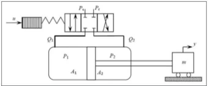
The positioning servo system driven by a hydraulic actuator considered here is depicted in Figure 1. The goal is to have the inertia load track any specified smooth motion trajectory as close as possible. The motion dynamics of the inertia load can be expressed as17m€y=P1A1P2A2By_AfSfð Þ y_ f y,ð y,_ tÞ ð1Þ
whereyandmrepresent the displacement and the iner-tial mass of the load, respectively;PL =P12P2is the
load pressure, whereP1andP2are the pressures inside
the two chambers of the cylinder; A1 and A2 are the
effective ram areas of the two chambers, respectively;B
represents the viscous friction coefficient, andAfSf
amplitude Af may be unknown but the continuous
approximated shape function Sf is known; f is the
lumped uncertain nonlinearities which cannot be mod-eled precisely due to nonlinear friction, external distur-bances, and other unmodeled dynamics.18
Neglecting the external leakage in the servo valve, pressure dynamics in actuator chambers can be written as19
_ P1=
be
V01+A1yðA1y_CtPL+Q1Þ _
P2= be V02A2y
A2y_+CtPLQ2
ð Þ
ð2Þ
wherebeis the effective oil bulk modulus;V01andV02
are the initial volumes of the two chambers, respec-tively;Ctis the coefficient of the total internal leakage
of the actuator;Q1is the supplied flow rate to the
for-ward chamber; and Q2 is the return flow rate of the
return chamber. Q1 and Q2 are related to the spool
valve displacement of the servo valve,xv, by11
Q1=kqxv s xvð Þ
ffiffiffiffiffiffiffiffiffiffiffiffiffiffiffiffi PsP1 p
+sðxvÞ ffiffiffiffiffiffiffiffiffiffiffiffiffiffiffiffi P1Pr p
h i
Q2=kqxv s xð Þv
ffiffiffiffiffiffiffiffiffiffiffiffiffiffiffiffi P2Pr p
+sðxvÞ
ffiffiffiffiffiffiffiffiffiffiffiffiffiffiffiffi PsP2 p
h i ð3Þ
wherekq=Cdwpffiffiffiffiffiffiffiffi2=rands(xv) is defined as
s xvð Þ= 10, if xv0 , if xv\0
ð4Þ
wherekqis the valve discharge gain,Cdis the discharge
coefficient,w is the spool valve area gradient, ris the density of oil,Psis the supply pressure of the fluid, and
Pris the return pressure.
In this article, it is assumed that the control applied to the servo valve is directly proportional to the spool position, then the following equation is given byxv=
kiu, wherekiis a positive electrical constant anduis the
input voltage.11Then, from equation (4),s(xv) =s(u).
Therefore equation (3) can be transformed to
Q1=gR1u
Q2=gR2u ð5Þ
whereg=kqkiand
R1=s uð Þ
ffiffiffiffiffiffiffiffiffiffiffiffiffiffiffiffi PsP1 p
+sðuÞ ffiffiffiffiffiffiffiffiffiffiffiffiffiffiffiffi P1Pr p
R2=s uð Þ ffiffiffiffiffiffiffiffiffiffiffiffiffiffiffiffiP2Pr p
+sðuÞ ffiffiffiffiffiffiffiffiffiffiffiffiffiffiffiffiPsP2
p ð6Þ
Assumption 1. In practical hydraulic system under normal working conditions, both P1 and P2 are
bounded byPrandPs,10that is, 0\Pr\P1\Ps and
0\Pr\P2\Ps.
Based on equations (1), (2), and (5), definex= [x1,
x2, x3]T= [y, y,_ A1P12A2P2]T as the system states.
Thus, the entire system can be expressed in a state– space form as
_ x1=x2
mx2_ =x3Bx2AfSfð Þ x2 dn~d x1,ð x2,tÞ
_ x3=
A1 V1R1+
A2 V2R2
gbeu A 2 1 V1 + A2 2 V2
bex2
A1 V1
+A2 V2
beCtPL
ð7Þ
where dn represents the lumped nominal value of the
unmodeled dynamics and external disturbances,20 ~
d(x1,x2,t) =f(x1,x2,t)dn.
In general, the system is subjected to structured uncertainties due to large variations in system para-metersm, B, Af, V01,V02,g,be, Ct, and so on. In
addi-tion, d(x~ 1,x2,t) is clearly the system unstructured uncertainty which cannot be modeled by an explicit function. For simplicity, we only consider the system parametersB, Af, dn, Ct, which are difficult to learn, as
the parametric uncertainties, and others are all known. Define the unknown but constant parameter set u= [u1, u2, u3, u4]T= [B, Af, dn, Ct]
T
. Then, equation (7) can be transformed to
_ x1=x2
m_x2=x3u1x2u2Sfð Þ x2 u3~d _
x3=g3ufcu4fu
ð8Þ
where
g3= A1 V1
R1+A2 V2
R2
gbe
fc= A2 1 V1 +A 2 2 V2
bex2
fu= A1 V1 +
A2 V2
bePL
ð9Þ
Assumption 2. Parametric uncertaintiesuand uncertain nonlinearitiesd~satisfy
u2Ou=fu:uminuumaxg ~
d xð 1,x2,tÞ
dd
ð10Þ
where umin= [u1min, ., u4min] T
; umax= [u1max, .,
u4max]T; andddis a known function.
Assumption 3. The desired position yd(t)=x1d(t) is C3
continuous and bounded.
RBF NN-based adaptive robust nonlinear
feedback controller design
Discontinuous projection mapping
Define u~=^uu as the estimation error, where ^u denotes the estimation ofu. A discontinuous projection is defined as9
Proj^u
ið Þi =
0, if^ui=uimaxandi.0 0, if^ui=uiminandi\0 i, otherwise
8 <
:
ð11Þ
wherei= 1, 2, 3, 4. In equation (11),i represents the
ith component of the vector , and the operation ‘‘\’’ for two vectors is performed in terms of the correspond-ing elements of the vectors. Suppose thatuis estimated using the following projection-type adaptation law
_^
u= Proj^uðG1t1Þ ^uð Þ 20 Ou ð12Þ
where Proj^u() =½Proj^u1(1),. . ., Proj^u4(4)T; G1.0
is a positive diagonal matrix, which denotes the para-meter adaptation gain; andt1is an adaptation function
to be synthesized in the controller design later. It can be shown that for any adaptation function t1, the above
projection mapping has the following properties21
P1
ð Þ u^2O^u=nu^:umin^uumaxg
P2
ð Þ u~T G11Proj^
uðG1t1Þ t1
0
ð13Þ
Controller design
Step 1. Noting that the first equation of equation (8) does not have any uncertainties, we can design in one step by combining the first two equations of equation (8). By introducingx2eqas the virtual control input for
x2, we can define the following error variables
z1=x1x1d
z2=z_1+k1z1=x2x2eq,x2eq=x_1dk1z1 ð 14Þ
wherek1is a positive feedback gain andz1denotes the
position tracking error. Since z1(s) =G(s)z2(s),
G(s) = 1/(s+k1) is a stable transfer function, making
z1converge to zero is equivalent to makingz2converge
to zero. Thus, the rest of the design is aimed to makez2
converge to zero. Now according to equations (8) and (14), we have
m_z2=m_x2m_x2eq=x3u1x2 u2Sfð Þ x2 u3~dmx_2eq
ð15Þ
Step 2. In this step, we considerx3as the virtual control
input and construct a control function a2 for x3 such
thatz2converges to zero, in which the transient
perfor-mance is also guaranteed. The control function a2 is
given by
a2=a2a+a2s
a2a=m_x2eq+^u1x2+^u2Sfð Þx2 +^u3+^~d a2s=a2s1+a2s2,a2s1= k2s1z2
ð16Þ
wherek2s1.0 is a feedback gain andd^~is the
approxi-mation of~d. In equation (16),a2ais the model
feedfor-ward compensation term through online parameter adaptation given by equation (12), a2s1 is the linear
robust feedback term to stabilize the system nominal model by adjustingk2s1, anda2s2is the nonlinear robust
feedback term to be synthesized later.22
Now, we need to design an approximator to approx-imate uncertain nonlinearities such as~dand designa2s2
to weaken simultaneously the parameter estimation error and uncertainty approximation error to stabilize the system. The two aspects of design processes are, respectively, as follows:
1. Given a sufficient number of hidden layer neu-rons and input information, the input–output mapping of RBF NN can be expressed as23 (structure chart is shown in Figure 2)
~
d=WTh xð Þ+eapprox ð17Þ
hjð Þx = exp
xcj 2 2b2
j !
ð18Þ
wherexis the input of RBF network;h(x) = [hj(x)]T is
Gaussian RBF, wherejdenotes thejth node of the hid-den layer;W*is the ideal weight of RBF network; and eapprox is the approximation error of RBF network,
which satisfies, respectively
W2OW= W:WminWWmax
eapprox
eN
ð19Þ
Takex= [x1,x2]Tas the input of the network, then
^~
d=W^Th xð Þ ð20Þ
whereW^denotes the estimation ofW*. The weight adaptation law is given by
_^
W= ProjW^ðG2t2Þ ð21Þ
where ProjW^() has the same form as Proj^u(), G2
denotes the weight adaptation velocity matrix, andt2
is an adaptation function to be designed later.
Definez3=x32a2as the input discrepancy, and by
substituting equation (16) into equation (15), we have
m_z2=z3k2s1z2+a2s2u2T~u+W~Th xð Þ eapprox ð22Þ
where W~=W^W denotes the estimation error of weights
u2= x2, Sfð Þx2 ,1,0
T
ð23Þ
is the regressor for parameter adaptation.9
2.a2s2, as a robust control law, is designed to
domi-nate the model uncertainties existed in the practical system, such as~u,W~, andeapprox.
Noting assumption 2, equation (19), andP1in
equa-tion (13), there existsa2s2 such that the following two
conditions are satisfied3
z2a2s20 ð24Þ
z2 a2s2uT2~u+W~ T
h xð Þ eapprox
h i
e2 ð25Þ
where e2 is a positive design parameter which can be
arbitrarily small.24
Here gives an example to choosea2s2to satisfy
con-straints such as equations (24) and (25)
a2s2= k2s2z2= h2
2 4e2
z2 ð26Þ
wherek2s2is a positive nonlinear gain andh2represents
the sum of the upper bounds of all errors, which means
uT2~u+W~ T
h xð Þ+eapprox
h2 ð27Þ
Step 3. This step is to synthesize an actual control law foru such thatz3converges to zero. Noting the third
equation of equation (8), we have
_
z3=x3_ a_2=g3ufcu4fua_2 ð28Þ
where
_
a2=a_2ca_2u
_ a2c=
∂a2 ∂t +
∂a2 ∂x1x2+
∂a2 ∂x2^_x2+
∂a2 ∂^u u_^+
∂a2 ∂W^ W_^
_ a2u=
∂a2 ∂x2~_
x2
^_ x2= 1
m x3^u1x2^u2Sfð Þ x2 ^u3d^~
~_ x2=
1 m u
T 2~uW~
T
h xð Þ+eapprox
ð29Þ
wherea_2cdenotes the calculable part ofa_2 and can be used in the design of the actual controlleruanda_2u is the incalculable part due to uncertainties which can be attenuated by the robust controller.
According to equations (28) and (29), the adaptive robust controlleruis given by
u=ua+us
ua= 1 g3
fc+^u4fu+a_2c
us= 1
g3ðus1+us2Þ,us1=k3s1z3
ð30Þ
where k3s1.0 is a feedback gain, ua functions as an
adaptive control law, and us as a robust control law.
By substituting equation (30) into equation (28), we have
_
z3=k3s1z3+us2+~u4fu+a_2u
=k3s1z3+us2+~u4fu
∂a2
∂x2 1
m~u1x2
∂a2
∂x2 1
m~u2Sfð Þx2
∂∂a2 x2 1
m~u3
∂a2
∂x2 1
m W~ T
h xð Þ eapprox
=k3s1z3+us2uT3~u
∂a2
∂x2 1
m W~ T
h xð Þ eapprox
ð31Þ
where
u3= 1 m
∂a2 ∂x2
x2, ∂a2 ∂x2
Sfð Þx2 , ∂a2 ∂x2
, mfu
T
ð32Þ
Similarly, one us2can be selected to satisfy the
fol-lowing two conditions3
z3us20 ð33Þ
z3 us2uT3~u ∂a2 ∂x2
1 m W~
T
h xð Þ eapprox
e3 ð34Þ
where e3 is a positive design parameter which can be
arbitrarily small.
Taking the design solution ofa2s2for reference, one
feasible example ofus2is given below
us2= k3s2z3= h3
2
4e3z3 ð35Þ
wherek3s2is a positive nonlinear gain and
uT3~u+ ∂a2
∂x2 1 m W~
T
h xð Þ+eapprox
h3 ð36Þ
Main results
Theorem 1. For any adaptation functiont1andt2, the
designed adaptive robust controller (30) has the follow-ing properties:
All signals in the closed-loop controller are bounded, and consider the Lyapunov function V3=(1=2)k12z21+(1=2)mz22+(1=2)z23which is bounded by
V3emtV3ð Þ0 + e m 1e
mt
½ ð37Þ
where e=e2+e3, m¼D 2lmin(L3) minf1=k
2
1,1=m,1g, andlmin(L3) is the minimum eigenvalue of the positive
definite matrixL3which is given by
L3=
k3
1
k12
2 0
k 2 1
2 k2s1 1 2
0 1
2 k3s1 2
6 6 6 6 6 4
3
7 7 7 7 7 5
ð38Þ
Theorem 2. With the discontinuous projection-type parameter adaptation law (12) and weight adaptation law (21) in whicht1andt2are chosen, respectively, as
t1=u2z2+u3z3 ð39Þ
t2= ∂a2 ∂x2
1 mz3z2
h xð Þ ð40Þ
then the control input (30) guarantees.
If after a finite time, the system is subjected to para-metric uncertainties only with RBF network–based ARC law (30) (i.e. ~d=WTh(x),25 namely,eapprox= 0
after a finite time), in addition to results in theorem 1,
asymptotic output tracking is also achieved,9 that is, z!0 ast!N, in whichz= [z1,z2,z3]T.
Proof. See Appendix 1.
Remark. From theorem 1, some theoretical results imply that the control strategy proposed can obtain an expected transient performance in the form of exponen-tial convergence and the final steady-state performance is also able to be guaranteed by adjusting certain con-troller parameters freely in a specified form. It is partic-ularly important to have such desired transient performance and final tracking precision, which are always the target of high-accuracy motion control sys-tems. Results achieved from theorem 2 reveal that, by way of utilizing parameter and weight adaptation laws, the parametric uncertainties may be restrained, and an enhanced steady performance is obtained to guarantee the stabilization of hydraulic servo systems.
Simulation results
To verify the performance of the proposed RBF NN-based adaptive robust controller (ARCNN), computer simulation has been carried out. The results are com-pared with those obtained from an adaptive robust controller and a proportional–integral–derivative (PID) controller. The three controllers are tested for a sinusoidal-like motion trajectory x1d= sint[12
exp(20.01t3)], and four cases are tested for this motion trajectory.
Case 1: normal case
Assuming no any disturbances from the external envi-ronment exist, by calculating the control inputuunder the integration of multiple control policies proposed, take the control input uinto account, which is directly implemented to the practical system.
Case 2: input disturbance case
By transforming the control input u into 0.5u, which indicates the input disturbance be loaded to the practi-cal system. So as to suppress strong structured uncer-tainties, this type of disturbance is applied, on one hand, which will product great influences on the rate of parameter/weight convergence and, on the other hand, which is used to examine the adaptive capacity of the proposed controller against input disturbances and the final tracking performance of control systems.
Case 3: position–velocity disturbance case
system, multiple disturbances integrated are applied by modifying the control inputuasu20.5x1x2. Exposed
to heavy unstructured uncertainties, the performance of system itself will bring about great changes, especially affectingd~greatly under this type of disturbance.
Case 4: position–velocity–input disturbance case
By synthesizing case 2 and case 3, the worst working condition is implemented to the practical physical sys-tem via loading 0.5u20.5x1x2 as the control input.
Similarly, this compound disturbance will exert great influences on the convergence of parameters and weights, together with ~d. Whether the proposed con-troller achieves a stable performance under this case or not, it can be viewed as the most comprehensive verifi-cation among all cases.
To illustrate the controller design, simulation results are obtained for the dynamic models of the hydraulic system discussed in section ‘‘Problem formulation and dynamic models,’’ with the following actual parameters:
Ps= 73 106Pa, Pr= 0 Pa, V01=V02= 131023m3,
A1=A2= 23 1024m2, m= 40 kg, B= 80 N s/m,
Ct= 73 10212m5/(N s), g= 431028m4/(s VON),
be= 2310 8
Pa, Af= 10 N, Sf= 2 arctan(1000y)=_ p,
anddn= 0 N. Thus, the actual value ofuisu= [80 10 0
7310212]T, and the uncertain nonlinearity term~d=0. The controller parameters are given, respectively, under the compared three controllers.
ARCNN. The control gains are chosen as k1= 250,
k2=k2s1+k2s2= 100, and k3=k3s1+k3s2= 50.
The bounds of parametric ranges are given by umin=
[60 220 250 4310212]T and umax= [100 20 50
103 10212]T. The initial estimation of u and W are ^
u(0) =½60 0 0 4 10 12T and W^(0) = ½ 10 10 10 10 10T, respectively. The parameter adaptation rates are set asG1= diag{50 20
13 102151310210} and the weight adaptation rates asG2= diag{10 10 10 10 10}. Parameters of RBF NN
are chosen asc= [20.820.4 0 0.4 0.8]Tandb= [5 5 5 5 5]T.
ARC. The control gains are chosen as k1= 100,
k2= 80, and k3= 50. The parameter adaptation rates
are set asG1= diag{100 30 50 1310230}. The other
controller parameters are the same as the correspond-ing parameters in ARCNN.
PID. PID controller, which is generally acted as a refer-ence controller for comparison, is commonly treated as a feedback-loop part in industrial control applications. Via an error-and-try mechanism, its control gains, which are chosen askp= 200,ki= 0, andkd= 50, can
be tuned carefully to maintain the stability of the system.
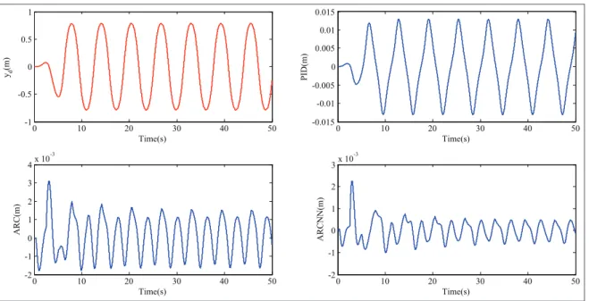
The desired motion trajectory and corresponding tracking performance under the three controllers in normal case are shown in Figure 3. According to this figure, we can conclude that the proposed ARCNN and ARC controllers have better transient and final tracking performance than the PID controller, which proves that employing ARC can estimate parameter uncertainties and compensate them in controllers. The PID controller just has some robustness against uncer-tainties, and its tracking error (about 0.013 m) is rela-tively large. Although ARC has some learning capability via parameter adaptation, the learning pro-cess makes no difference to uncertain nonlinearities
(i.e.~d). That is why the performance of ARC is worse than that of the controller with RBF. In addition to estimate uncertain parameters (parameter estimation is shown in Figure 4), the ARCNN controller can simul-taneously overcome structured and unstructured uncer-tainties with RBF NN, which greatly improves the tracking performance. This verifies the effectiveness of the proposed scheme with ARC and RBF NN. From Figure 1, the final tracking error of ARCNN is reduced down to 2.631024
m, while ARC has a larger track-ing error (about 3.731024
m).
To examine the effectiveness of the proposed algo-rithm against structured uncertainties, the simulation
under the input disturbance case is implemented with the same desired motion trajectory. The tracking errors of the three controllers are shown in Figure 5. In this case, the performance of ARC and ARCNN is much better than that of PID, whose tracking error (about 0.026 m) is greatly increased. The input disturbance, namely, structured uncertainties, can be captured by the adaptation law of ARCNN, and the residual distur-bances can be compensated by RBF NN. From the fourth figure, we can obtain that the maximal steady tracking error (about 3 31024
m) in ARCNN appears to be no much more different than that under normal case, which can also verify the effectiveness of the
Figure 4. Parameter estimation in normal case.
proposed controller with the combination of ARC and RBF NN.
To further examine the robustness of the proposed algorithm against unstructured uncertainties, the position–velocity disturbance case is taken into consid-eration, which will be the dominant factor affecting the tracking performance. The tracking errors of the three controllers are shown in Figure 6. As seen from this fig-ure, although faced with heavy unstructured uncertain-ties, the proposed ARCNN controller (maximal steady error of about 53 1024
m) is also able to weaken unexpected effects and achieves the best tracking per-formance among all three controllers. The parameter
estimation is presented in Figure 7. The estimation pro-cess ofuin ARCNN is unstable since the driving force of its parameter estimation is small; simultaneously, disturbed by this unstructured disturbance (disturbance and its estimation is shown in Figure 8), its learning capability is partially receded. In addition, the ARC controller exhibits worse performance than that shown previously due to the large position–velocity distur-bance (maximal steady error of about 1.531023
m). To farthest consider the authentic complex working conditions, the position–velocity–input disturbance is employed to examine the performance of the proposed controller. In this case, mixed with structured and
Figure 6. Tracking errors of the three controllers in position–velocity disturbance case.
unstructured uncertainties, all three controllers are affected at some extent. The tracking performance under this disturbance is shown in Figure 9. As seen, while there exists oscillation in the initial phase, the proposed ARCNN controller still achieves the satisfied tracking performance with a maximal steady tracking error of about 1 31023
m. It greatly proves the effec-tiveness of the proposed algorithm with RBF NN. Nevertheless, ARC has slightly insufficient abilities to deal with this severe disturbance very well and present the large tracking error (about 3.53 1023
m).
Conclusion
In this article, an integrated control strategy named an ARC with an RBF NN, which takes into consideration not only the parametric uncertainties but also the uncertain nonlinearities, has been put forward for a high-accuracy motion control system driven by a hydraulic actuator. Lyapunov stability theory, the tool which is used to provide performance guarantees of closed-loop systems, is a critical theoretical basis to analyze the stability of control systems. Extensive results obtained by simulation under four working
Figure 8. Disturbance and its estimation in position–velocity disturbance case.
conditions are used to testify the feasibility of the pro-posed control strategy, which indicates that by introdu-cing an RBF NN-based disturbance observer to ARC, although strong external disturbances exist in actual sys-tems, a desired transient tracking performance and the final tracking accuracy can also be guaranteed. By mer-ging the fundamental working mechanisms of the two control approaches, it proves to achieve better perfor-mance results than that of the single ARC approach, particularly in facing parameter uncertainties and strong external disturbances, the design idea which inspires us to explore the more effective controller design scheme and propel it to industrial utility as soon as possible.
Declaration of conflicting interests
The author(s) declared no potential conflicts of interest with respect to the research, authorship, and/or publication of this article.
Funding
The author(s) disclosed receipt of the following financial sup-port for the research, authorship, and/or publication of this article: This work was supported by the National Natural Science Foundation of China under grant 51505224, the Natural Science Foundation of Jiangsu Province in China under grant BK20150776, and the National Natural Science Foundation of China under grant 51305203.
References
1. Yao B, Bu F, Reedy J, et al. Adaptive robust motion control of single-rod hydraulic actuators: theory and experiments.IEEE/ASME T Mech2000; 5: 79–91. 2. Merritt HE. Hydraulic control systems. New York:
Wiley, 1967.
3. Yang G, Yao J and Le G. Adaptive robust control of DC motors with time-varying output constraints. In:
Proceedings of the 2015 34th Chinese control conference (CCC), Hangzhou, China, 28–30 July 2015, pp.4256– 4261. New York: IEEE.
4. Vossoughi R and Donath M. Dynamic feedback lineari-zation for electrohydraulically actuated control systems.
J Dyn Syst: T ASME1995; 117: 468–477.
5. Yao B and Tomizuka M. Adaptive robust control of SISO nonlinear systems in a semi-strict feedback form.
Automatica1997; 33: 893–900.
6. Yao B. High performance adaptive robust control of nonlinear systems: a general framework and new schemes. In:Proceedings of the IEEE conference on deci-sion and control, San Diego, CA, 10–12 December 1997, pp.2489–2494. New York: IEEE.
7. Chen Z, Yao B and Wang Q. Accurate motion control of linear motors with adaptive robust compensation of nonlinear electromagnetic field effect. IEEE/ASME T Mech2013; 18: 1122–1129.
8. Chen Z, Yao B and Wang Q.m-synthesis based adaptive robust control of linear motor driven stages with
high-frequency dynamics: a case study with comparative experiments.IEEE/ASME T Mech2015; 20: 1482–1490. 9. Yao J, Jiao Z and Ma D. Extended-state-observer-based
output feedback nonlinear robust control of hydraulic systems with backstepping. IEEE T Ind Electron 2014; 61: 6285–6293.
10. Yao J, Deng W and Jiao Z. Adaptive control of hydrau-lic actuators with LuGre model-based friction compensa-tion.IEEE T Ind Electron2015; 62: 6469–6477.
11. Yao J, Jiao Z and Ma D. A practical nonlinear adaptive control of hydraulic servomechanisms with periodic-like disturbances.IEEE/ASME T Mech2015; 20: 2752–2760. 12. Lewis FL. Neural network feedback control: work at
UTA’s automation and robotics research institute.
J Intell Robot Syst2007; 48: 513–523.
13. Herrmanna G, Lewis FL, Ge SS, et al. Discrete adaptive neural network disturbance feedforward compensation for non-linear disturbances in servo-control applications.
Int J Control2009; 82: 721–740.
14. Ren X, Lewis FL and Zhang J. Neural network compen-sation control for mechanical systems with disturbances.
Automatica2009; 45: 1221–1226.
15. Rovithakis GA. Tracking control of multi-input affine nonlinear dynamical systems with unknown nonlineari-ties using dynamical neural networks.IEEE T Syst Man Cy B1999; 29: 179–189.
16. Kostarigka AK and Rovithakis GA. Adaptive neural net-work tracking control with disturbance attenuation for multiple-input nonlinear systems.IEEE T Neural Networ
2009; 20: 236–247.
17. Yao J, Jiao Z and Ma D. High-accuracy tracking control of hydraulic rotary actuators with modeling uncertainties.
IEEE/ASME T Mech2014; 19: 633–641.
18. Deng W, Yao J and Jiao Z. Adaptive backstepping motion control of hydraulic actuators with velocity and acceleration constraints. In: Proceedings of the 2014 IEEE Chinese guidance, navigation and control conference (CGNCC), Yantai, China, 8–10 August 2014, pp.219– 224. New York: IEEE.
19. Guo K, Wei J and Tian Q. Disturbance observer based position tracking of electro-hydraulic actuator. J Cent South Univ T2015; 22: 2158–2165.
20. Hong Y and Yao B. A globally stable high-performance adaptive robust control algorithm with input saturation for precision motion control of linear motor drive sys-tems.IEEE/ASME T Mech2007; 12: 198–207.
21. Wang X, Wang S, Wang K, et al. Adaptive fuzzy robust control of a class of nonlinear systems via small gain the-orem. In:Proceedings of the 2012 10th IEEE international conference on industrial informatics, Beijing, China, 25–27 July 2012, pp.559–564. New York: IEEE.
22. Hu J, Qiu Y and Liu L. High-order sliding-mode obser-ver based output feedback adaptive robust control of a launching platform with backstepping. Int J Control. Epub ahead of print 2 March 2016. DOI: 10.1080/ 00207179.2016.1147604.
international commerce (CIMCA’06), Sydney, NSW Australia, 28 November–1 December 2006, p.6. New York: IEEE.
24. Liu S, Garimella P and Yao B. Adaptive robust precision motion control of a flexible system with unmatched model uncertainties. In:Proceedings of the 2005 American control conference (ACC), Portland, OR, 8–10 June 2005, vol. 2, pp.750–755. New York: IEEE.
25. Park J and Sandberg IW. Universal approximation using radial-basis-function networks. Neural Comput 1991; 3: 246–257.
26. Deng W, Luo C, Yao J, et al. Extended state observer based output feedback asymptotic tracking control of DC motors. In:Proceedings of the 2015 34th Chinese con-trol conference (CCC), Hangzhou, China, 28–30 July 2015, pp.4262–4267. New York: IEEE.
Appendix 1
Proof of theorem
From equations (14), (22), and (31), and noting condi-tions (25) and (34), the time derivative ofV3is
_ V3=k
2
1z1z1_ +z2m_z2+z3z3_ =z2z3k2s1z
2 2+k
2 1z1z2k
3 1z21
+z2 a2s2uT2~u+W~ T
h xð Þ eapprox
h i
k3s1z 2
3+z3 us2uT3~u ∂a2 ∂x2
1 m W~
T
h xð Þ eapprox
k13z 2 1+k
2
1z1z2k2s1z 2
2+z2z3k3s1z 2
3+e2+e3 ð41Þ
From equation (38), we have
_
V3 zTL3z+e lminð ÞL3 z 2 1+z
2 2+z
2 3
+eemV3 ð 42Þ
which leads to equation (37). Thus, V3 is globally
bounded, namely, z1, z2, and z3 are bounded.
According to assumption 3 and equation (14), it proves that x2_ eq is bounded. Also, we see that u^ and W^ are bounded, so it is apparent thata2is bounded and then
x3is bounded, namely, the statexis bounded. Fromt1
and t2 are bounded, we have that u_^ and W_^ are also
bounded. Thus, the bound ofa_2cis apparent. The con-trol inputuis thus bounded. This proves theorem 1.
Now taking theorem 2 into consideration, since there only exist parametric uncertainties in the system, we can define the Lyapunov function as follows
Vs=V3+ 1 2~u
TG1 1 ~u+
1 2W~
TG1
2 W~ ð43Þ
From equation (41), the time derivative ofVsis
_
Vs=V_3+~u T
G11u_^+W~ T
G21W_^ = k13z
2 1+k
2
1z1z2k2s1z 2
2+z2z3k3s1z 2 3 +z2 a2s2uT2~u+W~
T h xð Þ
h i
+z3 us2uT3~u ∂a2
∂x2 1 mW~
T h xð Þ
+~uTG11u_^+W~ T
G21W_^
ð44Þ
Noting conditions (24) and (33), we have
_ Vs k
3 1z
2 1+k
2
1z1z2k2s1z 2
2+z2z3k3s1z 2 3 uT2~uz2u
T 3~uz3+~u
T
G11u_^ +W~Th xð Þz2
∂a2 ∂x2
1 mW~
T
h xð Þz3+W~ T
G21W_^ = k13z
2 1+k
2
1z1z2k2s1z 2
2+z2z3k3s1z 2 3 +~uT G11u_^ðu2z2+u3z3Þ
h i
+W~T G21W_^ ∂a2 ∂x2
1 mz3z2
h xð Þ
ð45Þ
According to the properties of adaptation laws, not-ing the definitions oft1andt2, we have
_ Vs k
3 1z21+k
2
1z1z2k2s1z 2
2+z2z3k3s1z 2 3 +~uT G11Proj^uðG1t1Þ t1
+W~T G21ProjW^ðG2t2Þ t2
k3 1z2
1+k 2
1z1z2k2s1z 2
2+z2z3k3s1z 2 3 = zTL3z lminð ÞL3 z
2 1+z
2 2+z
2 3
¼D Q ð46Þ