ISSN 0101-8205 / ISSN 1807-0302 (Online) www.scielo.br/cam
Integrating Ridge-type regularization in fuzzy
nonlinear regression
R. FARNOOSH1∗, J. GHASEMIAN1 and O. SOLAYMANI FARD2 1School of Mathematics, Iran University of Science and Technology,
Narmak, Tehran 16844, Iran
2School of Mathematics and Computer Science, Damghan University, Damghan, Iran E-mails: [email protected] / [email protected] / [email protected]
Abstract. In this paper, we deal with the ridge-type estimator for fuzzy nonlinear regression
models using fuzzy numbers and Gaussian basis functions. Shrinkage regularization methods are used in linear and nonlinear regression models to yield consistent estimators. Here, we propose a weighted ridge penalty on a fuzzy nonlinear regression model, then select the number of basis functions and smoothing parameter. In order to select tuning parameters in the regularization method, we use the Hausdorff distance for fuzzy numbers which was first suggested by Dubois and Prade [8]. The cross-validation procedure for selecting the optimal value of the smoothing parameter and the number of basis functions are fuzzified to fit the presented model. The simulation results show that our fuzzy nonlinear modelling performs well in various situations.
Mathematical subject classification: Primary: 62J86; Secondary: 62J07.
Key words:fuzzy nonlinear regression, regularization method, Monte Carlo method, Gaussian
basis expansion.
1 Introduction
Finding the relationships if any, existing in a set of variables when at least one is random, is known as an important task in statistics. On one hand, regression analysis, especially nonlinear regression, is an essential tool to analyze data.
Many researchers use nonlinear regression more than any other statistical tool. Nonlinear models have been applied to a wide range of situations, even to finite populations. These models tend to be used either when they are suggested by theoretical considerations or to build known nonlinear behavior into a model (see for example [22, 27, 30]).
On the other hand, in most statistical practices, particularly in biology, business or government, the underlying processes are generally complex and not well understood. Also, a model obtained as the solution of a differential equation generating from engineering, chemistry, or physics is usually nonlinear. Much applied work using linear models represents a distortion of the underlying subject matter. This means that we have no idea about the form of the relationship (see [12, 27]). One of the major advantages in using nonlinear regression is the wide range of functions that can be fit.
In many practical situations, it may be unrealistic to predetermine a fuzzy para-metric regression especially for a large data set with a complicated underlying variation trend. In this respect, some other approaches have been developed to deal with the fuzzy regression problems without predefining a specific form of the underlying regression relationship or with a nonlinear form of regression relationship.
The multicolinearity [21] among the independent variables leads to increasing error in estimating of regression coefficients. Shrinkage estimators have been developed for many situations including the linear and nonlinear regression mod-els. To yield consistent estimators, the nonlinear models, instrumental variables estimation seems necessary. For this reason, the use of shrinkage estimation to nonlinear settings is recommended. The Poisson regression model [25] and the probit model [1] as well as to the Box-Cox transformation [18] are cases of such models. These papers provide theoretical results indicating the superior performance in terms of risk of certain shrinkage estimators over unrestricted estimation [10].
structures. Expressing regression functions as a linear combination of known nonlinear functions called basis functions is the main purpose in basis expan-sions. However, natural cubic splines, B-splines, Fourier series and radial basis functions are widely used as basis functions [24]. In the current study, we use Gaussian basis functions [4] because they can be expressed in a simple form and can be easily implemented. When Gaussian basis functions are constructed for unequally spaced data, narrow basis functions with very small dispersions might be constructed, which can unsmoothing or unstable results if we employ these bases. Therefore, to overcome this problem, a shrinkage estimation, which allows to avoid these effects on the narrow basis functions by estimating their coefficients towards exactly zero can be used [29].
The structure of paper is as follows: Section 2 explains basic concepts of fuzzy numbers which we used in this paper. In Section 3, multivariate fuzzy nonlinear regression model based on ridge estimation will be presented. In Sec-tion 4, we discuss the selecSec-tion of number basis funcSec-tions and the smoothing parameter. Finally, in the last two sections, some numerical examples and com-ments are given.
2 Preliminaries
In this section, we read some definitions and introduce the notations which will be used throughout the paper.
Definition 2.1.([3])Let X be a nonempty set. A fuzzy setu in X is characterized˜ by its membership functionu˜ :X → [0,1]. For each x ∈ X ,u˜(x)is interpreted as the degree of membership of an element x in the fuzzy setu.˜
Let us denote byRFthe class of fuzzy subsets of the real axis R(i.e. u˜ :R→
[0,1]) satisfying the following properties:
(i) u˜ is normal,i.e., there existss0∈ Rsuch thatu˜(s0)=1,
(ii) u˜ is a convex fuzzy set,i.e.,
˜
u(ts+(1−t)r)≥min{ ˜u(s),u˜(r)}, ∀t∈ [0,1], s,r ∈ R
(iii) u˜ is upper semi-continuous onR,
RF is called the space of fuzzy numbers, and obviously R⊂ RF.
For 0 < α ≤ 1 denote [ ˜u]α
= {s ∈ R | ˜u(s)≥α} and [ ˜u]0
= cl{s ∈ R | ˜u(s) >0}. It is clear that theα−level set of a fuzzy number is a closed and bounded interval[uα,uα], whereuα denotes the left-hand endpoint of[ ˜u]α and uαdenotes the right-hand endpoint of[ ˜u]α.
Another definition for a fuzzy number is as follows.
Definition 2.2. ([3]) A fuzzy number u in parametric form is a pair˜ (u,u) of functions u(α), and u(α), 0 ≤ α ≤ 1, which satisfies the following require-ments:
(i) u(α)is a bounded non-decreasing left continuous function in(0,1], and right continuous at0,
(ii) u(α)is a bounded non-increasing left continuous function in(0,1], and right continuous at0,
(iii) u(α)≤u(α),0≤α ≤1.
A crisp number a is simply represented byu(α) = u(α) = a,0 ≤ α ≤ 1. We recall that fora < b <c, whicha,b,c ∈ R, the triangular fuzzy number
˜
u=(a,b,c)determined bya,b,cis given such thatu(α)=a+(b−c)αand ¯
u(α)=c−(c−b)αare the endpoints of theα-level sets, for allα∈ [0,1].
For arbitraryu˜ =(u(α),u(α)),v˜ =(v(α), v(α)), we define the following
(i) (u˜⊕ ˜v)(α)=(u(α)+v(α),u(α)+v(α)),∀α ∈ [0,1],
(ii) (u˜− ˜v)(α)=(u(α)−v(α),u(α)−v( α)),∀α ∈ [0,1],
(iii) (k⊗ ˜u)(α)=
(
(ku(α),ku(α)),k ≥0
(ku(α),ku(α)),k <0 ,∀α ∈ [0,1],
wherekis a scalar. Moreover, whenk = −1, we havek⊗ ˜u = − ˜u.
The Hausdorff distance between fuzzy numbers given by D : RF ×RF →
R+S
{0},
D(u˜,v)˜ = sup α∈[0,1]
max u(α)−v(α)
,|u(α)−v(α)| ,
Note that (RF,D) is a complete metric space (see [3, 11, 13]) and has the
following properties,
(i) D(u˜⊕ ˜w,v˜⊕ ˜w)=D(u˜,v),˜ ∀ ˜u,v,˜ w˜ ∈ RF,
(ii) D(k⊗ ˜u,k⊗ ˜v)= |k|D(u˜,v),˜ ∀k ∈ R,u˜,v˜ ∈ RF,
(iii) D(u˜⊕ ˜v,w˜ ⊕ ˜e)≤ D(u˜,w)˜ +D(v,˜ e˜),∀ ˜u,v,˜ w,˜ e˜ ∈ RF.
Definition 2.3. ([3]) A mapping f : RF → RF is called a fuzzy process.
Therefore, itsα-level set can be written as follows,
[f(x˜)]α = [fα(x˜), fα(x˜)],x˜ ∈ RF, α ∈ [0,1].
Definition 2.4. ([11])A mapping f : RF → RF is called continuous at point
˜
x0 ∈ RF provided for any fixedα ∈ [0,1] and arbitraryε > 0, there exists δ(ε, α)such that D([f(x˜)]α,[f(x0˜ )]α) < ε, whenever D([ ˜x]α,[ ˜x0]α) < δ(ε, α)
for allx˜ ∈ RF.
3 Multivariate Fuzzy Nonlinear Regression Model Based on Ridge Estimation
A fuzzy nonlinear regression model with multivariate fuzzy input and output is considered in this section and, a fitting procedure is proposed for this model.
Suppose that we haven independent observations (y˜i,x˜i);i = 1,2, . . . ,n.
Here, a fuzzy nonlinear regression model is considered as follows,
˜
yi =m(x˜i)⊕ ˜εi,i =1,2, . . . ,n (1)
In this model, x˜i = (x˜i1, . . . ,x˜i p) ∈ (RF)p; i = 1,2, . . . ,n, are vectors of
p-dimensional independent variables(inputs) and y˜i ∈ RF is univariate output.
The functionm(.), a mapping from(RF)pto RF, is an unknown fuzzy smooth
function. Moreover,εi˜ ∈ RFfor whichε˜iα =(εi(α), εi(α)), andεi(α)andεi(α))
are independently, normally distributed with mean zero and variance σ2(α). Regarding Definition 2.3, the fuzzy functionm(.)can be expressed as
mα(x˜i j)=
mα(xi j),mα(xi j)
So, we can write the modely˜ =m(x˜)⊕ ˜ε, as the follow form,
y(α)=mα(x˜) +ε(α)
y(α)=mα(x˜)+ε(α)
(2)
that equivalent to
y(α)=m(x,x;α)+ε(α)
y(α)=m(x,x;α)+ε(α)
(3)
We may assume any component ofm(.)orm(.)has a linear combination of basis functionsφl(x,x, α);l=1, . . . ,kin the form
m(x,x, α)=b0(α)+ k
X
l=1
bl(α)φl(x,x, α) (4)
and
m(x,x, α)=b0(α)+ k
X
l=1
bl(α)φl(x,x, α) (5)
where
b(α)=(b0(α),b1(α), . . . ,bk(α))T andb(α)=(b0(α),b1(α), . . . ,bk(α))T
are fuzzy unknown coefficient parameter vectors and forXα =(x,x, α), Gaus-sian basis functions are given by
φl(Xα,µ
l(α),hl(α))=exp
−||X
α−µ
l(α)|| 2
2h2 l(α)
,
φl(Xα,µl(α),hl(α))=exp
−||Xα−µl(α)||2
2h2l(α)
,
(l=1, . . . ,k) (6)
whereµ
l(α)andµl(α)are p-dimensional vector determining the center of the
basis functions,hl2(α)andhl
2
(α)are the width parameters and||.||is the Euclid-ian norm. Unknown parameters in the models (4) and (5) include the coefficient parametersb(α)=(b(α),b(α)), and the centersµ
l(α),µl(α)and width
param-etershl2(α),hl
2
and identification problems. In the first stage, the centersµ
l(α),µl(α)and
dis-persionhl2(α),hl
2
(α)are determined by using thek-means clustering algorithm. The data set of observations of the explanatory variables(x1(α), . . . ,xn(α))and (x1(α), . . . ,xn(α))are divided respectively intok clusters(C1(α), . . . ,Ck(α))
and(C1(α), . . . ,Ck(α)); centersµl(α),µl(α)and dispersionshl2(α),hl
2 (α)are determined by ˆ µ
l(α)=
1
nl
P
xi(α)∈Cl xi(α),
ˆ
µl(α)= n1l
P
xi(α)∈Cl xi(α),
ˆ h2l(α)= n1
l
P
xi(α)∈Cl||xi(α)−μl(α)||2,
ˆ
h2l(α)= n1
l
P
xi(α)∈Cl||xi(α)−µl(α)||
2,
(l=1, . . . ,k) (7)
wherenl is the number of observations included in thel-th cluster Cl or Cl .
Replacingμl(α) = (µl(α),µl(α))andh2l(α) =(hl2(α),hl
2
(α))in (6) by (7) respectively, we obtain a set of 2kbasis functions
φl(Xα,µˆl(α),hˆl(α))=exp
−||Xα− ˆµl(α)|| 2
2hˆ2l(α)
,
φl(Xα,µˆl(α),hˆl(α))=exp
−||Xα− ˆµl(α)||2
2hˆ2l(α)
,
(l=1, . . . ,k) (8)
Forn independent observations(y˜i,x˜i);i =1,2, . . . ,n,the fuzzy nonlinear
regression model based on Gaussian basis functions
φl(Xα,µ
l(α),hl(α)), φl(X
α
,µl(α),hl(α)),l=1, . . . ,k
given in (6) is expressed as
y
i(α)=b
T(α)φ (Xα
i,µl(α),hl(α))+εi(α)
yi(α)=b T
(α)φ (Xα
i,µl(α),hl(α))+εi(α)
(9)
where
φ(Xαi,µl(α),hl(α))=(1, φ1(Xαi,µl(α),hl(α)), . . . , φk(X
α
i,µl(α),hl(α))),
andεi(α), εi(α)are error terms. If the error terms are independently and
nor-mally distributed with mean 0 and varianceh2
l(α) = (hl
2
(α),hl
2
(α)), for all
α∈ [0,1]the nonlinear regression model (9) has a probability density function
f y
i(α)|X
α
i;b(α),h
2
(α)
= √ 1
2πh2(α)exp
−{yi(α)−b T(α)φ(Xα
i)} 2
ˆ
2h2(α)
,
f
yi(α)|Xiα;b(α),h
2
(α)
= √ 1 2πh2(α)
exp
−{yi(α)−b T
(α)φ(Xαi)}2
ˆ
2h2(α)
, (i =1, . . . ,n)
(10)
Then the maximum likelihood estimates of the coefficient vectorsb(α),b(α)
andh2
l(α)=(hl2(α),hl
2
(α))are respectively given by
ˆ
b(α)=(8T8)−18Ty(α)
ˆ
b(α)=(8T8)−18Ty(α) ˆ
h2(α)= n1[y(α)−8bˆ(α)]T[y(α)−8bˆ(α)]
1
n[y(α)−8bˆ(α)] T
[y(α)−8bˆ(α)]
(11)
where
8=(φ (Xα1,µ
l(α),hl(α)), . . . , φ (X
α
n,µl(α),hl(α))),
8=(φ (Xα1,µl(α),hl(α)), . . . , φ (Xαn,µl(α),hl(α))), y(α)=(y
1(α),y2(α), . . . ,yn(α)) T,
y(α)=(y1(α),y2(α), . . . ,yn(α))T.
We estimate b(α) = (b(α),b(α)) and h2(α) by the regularization method, because the maximum likelihood method often yields unstable estimates in fitting a nonlinear model to data with a complex structure. We consider maximizing the penalized log-likelihood function, instead of using the log-likelihood function,
lλ(θ(α))=Pn
i=1log f y α
i|X
α
i;b(α),h(α)
−nλH(b(α))
lλ(θ (α))=Pn
i=1log f y α
i|X
α
i;b(α),h(α)
−nλH(b(α))
where
θ (α)=(bT(α),h2(α))T, θ (α)=(bT(α),h2(α))T,
andH(b(α))= [H(b(α)),H(b(α))]is a penalty function forb(α)andλ(>0)
is a smoothing parameter that controls the smoothness of the fitted model. Based on the ridge penalty, inl2norm,(H(b(α)),H(b(α)))given by
H(b(α))= 12 Pk l=1bl
2(α) = 1
2b
T(α)b(α),
H(b(α))= 12 Pk l=1bl
2
(α)= 12bT(α)b(α).
(13)
Then, the maximum penalized likelihood estimates ofb(α)=(b(α),b(α))and h2(α)
=(h2(α),h2(α))are respectively given by
ˆ
b(α)= [8T8+nλhˆ2(α)Il+1]−18Ty(α), ˆ
b(α)= [8T8+nλhˆ 2
(α)Il+1]−18
T y(α),
ˆ
h2(α)= 1n[y(α)−8bˆ(α)]T[y(α)−8bˆ(α)],
ˆ h 2
(α)= 1n[y(α)−8bˆ(α)]T[y(α)−8bˆ(α)].
(14)
Il+1 is an (l +1) dimensional identity matrix. Note that these estimators depend on each other. Therefore, we provide an initial value for the variance
h2X˜α(0)(α),h
2
˜
Xα(0)(α)
first, then(bˆ(α),bˆ(α))and
h2X˜α(α),h
2
˜
Xα(α)
are up-dated until convergence. This estimation method is the maximum penalized likelihood with the quadratic form (see [9, 23]). The consistency and the rate of convergence of these estimators proved in ([5, 15, 20]).
4 Selection of the number of basis function and the smoothing parameter
The estimates that achieved in(14)by the regularization method depends upon the number of basis functions 2k and the value of the smoothing parameterλ. Appropriate determining these values is a crucial issue. The fuzzified cross-validation procedure based on the Hausdorff distance between fuzzy numbers, can be described as follows. Let
ˆ y
i(α)= ˆm
α
(x˜i)= ˆb T
(α)φ(Xαi,µ
l(α),hl(α))
ˆ
yi(α)= ˆmα(x˜i)= ˆb T
(α)φ(Xαi,µl(α),hl(α)),
be the predicted fuzzy ridge nonlinear regression function at inputXiαcomputed by our method. Let
C V(k, λ)=1
n
n
X
i=1
D(y˜i,yˆ˜i). (16)
TheC V(k, λ)quantity gives an overall measurement of the difference between the actual values of dependent variable and its estimation. However, because of the error term in model (1) the C V(k, λ) cannot efficiently reflect the close-ness between the underlying fuzzy nonlinear regression functionm(x˜)and its estimate. Therefore, we define a quantity for measuring the bias between the objective function and its estimate, which is
B I AS(k, λ)=1
n
n
X
i=1
D(m(x˜i),mˆ(x˜i)). (17)
The B I AS(k, λ)makes sense for examining the performance of the different methods by simulation. BothC V(k, λ)andB I AS(k, λ)will be reported in our simulations to numerically evaluate the performance of the proposed method. Choosek0andλ0as the optimal values such that
C V(k0, λ0)= min
k>0,λ>0C V(k, λ), and, B I AS(k0, λ0)= min
k>0,λ>0B I AS(k, λ).
In practice, we may compute for a series of values ofk andλto obtaink0and
λ0. A smoother regression function generally corresponds to a larger value ofk while a more fluctuating regression function tends to select a smaller value ofk.
5 Numerical results
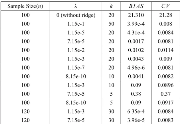
In this section, we use Monte Carlo simulations to investigate the performance of the proposed model by computing C V(k, λ) and B I AS(k, λ). Here, two simulation examples are considered: a curve fitting and a surface fitting. The results are obtained for some values of sample size,kandλ.
Example 5.1.Curve fitting. In this simulation repeated random samples(y˜i,x˜i);
regression modely˜i =m(x˜i)⊕ ˜εi where
m(x˜)=exp(2x˜2).
The design points x˜i are uniformly distributed in [0,1]F ⊆ RF and the
errorsε˜αi =(εi(α), εi(α)), whichεi(α)andεi(α)are independently, normally distributed. The mean of distribution is zero and the standard deviations are respectivelyτ =0.1Rm andτ =0.1Rm with Rm,Rm being the ranges ofm(x˜)
orm(x˜)overx˜i ∈ [0,1]F.
C V(k, λ)and B I AS(k, λ)are used to numerically evaluate the performance of method and the related results are summarized in Table 1. In this example it is clear that the ridge estimation must be used.
Sample Size(n) λ k B I AS C V
100 0 (without ridge) 20 21.310 21.28
100 1.15e-1 50 3.99e-4 0.008
100 1.15e-5 20 4.31e-4 0.0084
100 7.15e-5 20 0.0017 0.0081
100 1.15e-2 20 0.0102 0.0114
100 1.15e-3 20 0.0043 0.009
100 1.15e-7 20 4.96e-6 0.0081
100 8.15e-10 10 0.0041 0.0082
100 1.15e-3 10 0.09 0.0896
100 7.15e-5 5 0.38 0.37
100 8.15e-10 5 0.09 0.0917
120 1.15e-3 30 6.35e-4 0.0084
120 7.15e-5 30 3.96e-5 0.0083
Table 1 – The simulation results obtained by the proposed method.
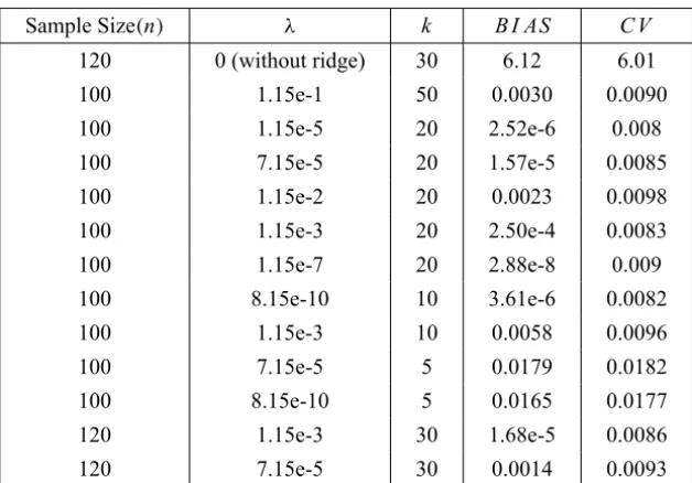
Example 5.2.Surface fitting. Next, we applied the modeling strategy to surface data. We generated random samples(y˜i,x1˜i,x2˜i);i =1,2, . . . ,nwithn=100
or 120 from a true modely˜i =m(x1˜i,x2˜i)⊕ ˜εi where
m(x1˜,x2˜)=exp
−2
q
˜
x12+ ˜x22
The design points(x1˜i,x2˜i)are uniformly distributed in[0,1]F × [0,1]F ⊆ (RF)2. The errorsε˜iα =(εi(α), εi(α)), whichεi(α)andεi(α)are independently,
normally distributed. The mean of distribution is zero and the standard devia-tions are respectivelyτ =0.1Rm andτ =0.1Rm withRm,Rmbeing the ranges
ofm(x1˜,x2˜)orm(x1˜,x2˜)over(x1˜,x2˜)∈ [0,1]F× [0,1]F.
Table 2 shows the result for this dataset. The results show that the ridge method still produces a quite satisfactory estimate of the fuzzy nonlinear regression in the case of two-dimensional input.
Sample Size(n) λ k B I AS C V
120 0 (without ridge) 30 6.12 6.01
100 1.15e-1 50 0.0030 0.0090
100 1.15e-5 20 2.52e-6 0.008
100 7.15e-5 20 1.57e-5 0.0085
100 1.15e-2 20 0.0023 0.0098
100 1.15e-3 20 2.50e-4 0.0083
100 1.15e-7 20 2.88e-8 0.009
100 8.15e-10 10 3.61e-6 0.0082
100 1.15e-3 10 0.0058 0.0096
100 7.15e-5 5 0.0179 0.0182
100 8.15e-10 5 0.0165 0.0177
120 1.15e-3 30 1.68e-5 0.0086
120 7.15e-5 30 0.0014 0.0093
Table 2 – The simulation results for two-dimensional dataset obtained by the proposed method.
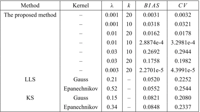
Example 5.3. Consider the below function from [31].
g(x)=10+5 sin(0.25π(1−x2))
Let
yi =g(xi)+rand[−0.5,0.5],
σi = 13g(xi)+rand[−0.25,0.25],
i=1,2, . . . ,100,
The observed fuzzy outputs are
˜
Table 3 shows the result for this dataset.
Method Kernel λ k B I AS C V
The proposed method – 0.001 20 0.0031 0.0032
– 0.001 10 0.0318 0.0321
– 0.01 20 0.0162 0.0178
– 0.01 10 2.8874e-4 3.2981e-4
– 0.03 10 0.2692 0.2944
– 0.03 20 0.1758 0.1982
– 0.003 20 2.2701e-5 4.3991e-5
LLS Gauss 0.21 – 0.0520 0.2252
Epanechnikov 0.52 – 0.0552 0.2544
KS Gauss 0.15 – 0.0821 0.2080
Epanechnikov 0.34 – 0.0848 0.2337 Table 3 – The simulation results obtained by different methods.
In this example LLS and KS, respectively stand for the local linear smoothing and kernel smoothing methods.
6 Conclusions
In this study, we dealt with estimating the ridge regularization in fuzzy non-linear regression model with modelling the data with multivariate fuzzy input and output. The ridge estimation of fuzzy nonlinear regression models based on Gaussian basis function with the cross-validation procedure for selecting the optimal values of the smoothing parameter and the number of basis function was proposed. Some simulation experiments were conducted to assess the perfor-mance of the method. By computing theC V(k, λ)andB I AS(k, λ), we found that the proposed method performs quite well in reducing the error and producing a satisfactory estimate of the parameters of nonlinear regression function.
As demonstrated by the numerical experiments, the increasing ofk, the number of basis function, increases the accuracy of model. In this case we can decrease the smoothing parameter λ. The small values of C V(k, λ) and B I AS(k, λ)
Acknowledgements. The authors are grateful to the associate editor and two referees for their accurate reading and their helpful suggestions and remarks.
REFERENCES
[1] L.C. Adkins and R.C. Hill, Risk characteristics of a Stein-like estimator of the probit regression model. Economics Letters,30(1989), 19–26.
[2] D.M. Bates and D.G. Watts, Nonlinear Regression Analysis and its Applications. Wiley, New York (1988).
[3] B. Bede and S.G. Gal,Generalizations of the differentiability of fuzzy umber valued functions with applications to fuzzy differential equation. Fuzzy Sets and Systems,
151(2005), 581–599.
[4] C.M. Bishop, Neural Networks for Pattern Recognition. Oxford University Press, Oxford (1995).
[5] D.D. Cox and F. O’Sullivan, Asymptotic Analysis of Penalized Likelihood and Related Estimators. Ann. Statist.,18(1990), 1676–1695.
[6] P. Diamond,Fuzzy least squares. Information Sciences,46(1988), 141–157. [7] N.R. Draper and H. Smith, Applied Regression Analysis. Wiley, New York (1980). [8] D. Dubois and H. Prade,Fuzzy Numbers: An Overview, Analysis of Fuzzy
Infor-mation. Mathematical Logic,CRC Press, Boca Raton, FL,1(1987), 3–39. [9] P.P.B Eggermont and V.N. Lariccia, Maximum Penalized Likelihood Estimation,
Springer (2001).
[10] S. Ejaz Ahmed and C.J. Nicol, An application of shrinkage estimation to the nonlinear regression model. Journal of Computational Statistics and Data Analysis (to appear).
[11] M. Friedman, M. Ma and A. Kandel,Numerical solutions of fuzzy differential and integral equations. Fuzzy Sets and Systems,106(1999), 35–48.
[12] A.R. Gallant, Nonlinear Statistical Models. Wiley, New York (1987).
[13] R. Goetschel and W. Voxman,Topological properties of fuzzy number. Fuzzy Sets and Systems,10(1983), 87–99.
[14] R. Goetschel and W. Voxman,Elementary fuzzy calculus, Fuzzy sets and Systems,
18(1986), 31–43.
[16] T.J. Hastie and R.J. Tibshirani, Generalized additive models, Chapman & Hall, London (1990).
[17] A.E. Hoerl and R.W. Kennard,Ridge regression: biased estimates for nonorthog-onal problems. Technometrics,12(1970), 55–67.
[18] M. Kim and R.C. Hill,Shrinkage estimation in nonlinear models. The Box-Cox transformation. Journal of Econometrics,66(1995), 1–33.
[19] B. Kim and R.R. Bishu,Evaluation of fuzzy linear regression models by comparing membership functions. Fuzzy Sets and Systems,100(1998), 343–352.
[20] G.A. Latham and S. Yu, N-Stage Splitting for Maximum Penalized Likelihood Estimation with Gaussian Data and Stationary Linear Iterative Methods. J. Statist. Comput. and Simul.,62(1999), 375–393.
[21] R.X. Liu, J. Kuang, Q. Gong and X.L. Hou, Principal component regression analysis with SPSS. Computer Methods and Programs in Biomedicine,71(2003), 141–147.
[22] H. Motulsky and A. Christopoulos, Fitting Modeles to Biological Data using Lin-ear and NonlinLin-ear Regression. GraphPad Software, Inc., San Diego (2003). [23] T. Poggio and F. Girosi, Networks for approximation and learning. Proc. IEEE,
78(1990), 1484–1487.
[24] D. Ruppert, M.P. Wand and R.J. Carrol, Semiparametric Regression, Cambridge University Press (2003).
[25] S.K. Sapra,Pre-test estimation in Poisson regression model. Applied Economics Letters,10(2003), 541–543.
[26] C. Saunders, A. Gammerman and V. Vork,Ridge regression learning algorithm in dual variable. Proceedings of the 15th International Conference on Machine Learning, (1998), 515–521.
[27] G.A.F. Seber and C.J. Wild, Nonlinear Regression. Wiley, New York (1989). [28] H. Tanaka and H. Ishibuchi, Identification of possibilistic linear systems by
quadratic membership functions of fuzzy parameters. Fuzzy Sets and Systems,
41(1991), 145–160.
[29] S. Tateishi, H. Matsui and S. Konishi,Nonlinear regression modeling via the lasso-type regularization. Journal of Statistical Planning and Inference, 140 (2010), 1125–1134.
[31] N. Wang, W.X. Zhang and C.L. Mei,Fuzzy nonparametric regression based on local linear smoothing technique. Information Sciences,177(2007), 3882–3900. [32] M. Yang and H. Liu,Fuzzy least squares algorithms for interactive fuzzy linear