Influence of gear loss factor on the power loss prediction

(1)

www.mech-sci.net/6/81/2015/ doi:10.5194/ms-6-81-2015

Influence of gear loss factor on the power loss prediction

C. M. C. G. Fernandes1, P. M. T. Marques1, R. C. Martins1, and J. H. O. Seabra2

1_{INEGI, Universidade do Porto, Campus FEUP, Rua Dr. Roberto Frias 400, 4200-465 Porto, Portugal} 2_{FEUP, Universidade do Porto, Rua Dr. Roberto Frias s/n, 4200-465 Porto, Portugal}

Correspondence to:C. M. C. G. Fernandes ([email protected])

Received: 29 October 2014 – Revised: 27 May 2015 – Accepted: 25 June 2015 – Published: 03 July 2015

Abstract. In order to accurately predict the power loss generated by a meshing gear pair the gear loss factor must be properly evaluated. Several gear loss factor formulations were compared, including the author’s approach.

A gear loss factor calculated considering the load distribution along the path of contact was implemented. The importance of the gear loss factor in the power loss predictions was put in evidence comparing the predic-tions with experimental results. It was concluded that the gear loss factor is a decisive factor to accurately predict the power loss. Different formulations proposed in the literature were compared and it was shown that only few were able to yield satisfactory correlations with experimental results. The method suggested by the authors was the one that promoted the most accurate predictions.

1 Introduction

According to Kragelsky et al. (1982) tribology is an im-portant field in engineering which can contribute to develop more reliable and efficient mechanisms like gearboxes.

According to Höhn et al. (2009) the power loss in a gear-box consists of gear, bearing, seals and auxiliary losses. Gear and bearing losses can be separated in no-load and load losses. No-load losses occur with the rotation of mechani-cal components, even without torque transmission. No-load losses are mainly related to lubricant viscosity and density as well as immersion depth of the components on a sump lu-bricated gearbox, but it also depends on operating conditions and internal design of the gearbox casing. Rolling bearing no-load losses depend on type and size, arrangement, lubri-cant viscosity and immersion depth.

Load dependent losses occur in the contact of the power transmitting components. Load losses depended on the trans-mitted torque, coefficient of friction and sliding velocity in the contact areas of the components. Load dependent rolling bearing losses also depend on type and size, rolling and slid-ing conditions and lubricant type (SKF, November 2005).

At nominal loads the power loss generated in a gearbox is mainly dependent of the gears load power losses, which puts in evidence the importance of the evaluation of the gear loss factor.

This work shows the influence of the gear loss factor for-mulation (considering different gear geometries) in the pre-diction of the power loss. The gear loss factor formulations will be compared with experimental results previously pub-lished by Fernandes et al. (2015).

2 Load dependent power loss in meshing gears

Ohlendorf (1958) introduced an approach for prediction of the load dependent losses on spur gears. The power loss gen-erated between gear tooth contact can be calculated accord-ing to Eq. (1),

PV ZP =PIN·HV·µmZ. (1)

HV is the gear loss factor.

Originally Eq. (1) was obtained assuming a constant co-efficient of friction (µmZ). This was a simplification of the

problem.

Equation (1) can be used to calculate the average power loss between gear teeth, given the correct gear loss factor HV. Despite consideringβbthe Eq. (2) initially proposed by

(2)

H_VOhl=(1+u)· π

z1

· 1

cosβb

·1−ǫα+ǫ12+ǫ22

(2)

The classical formulas for gear loss factor (Eqs. 3 and 4) con-sider a rigid load distribution, and a constant coefficient of friction, but tooth profile modifications are disregarded. In depth details about these formulas can be found in the clas-sical works of Niemann and Winter (1989) and Buckingham (1949).

Niemann and Winter (1989) proposed the gear loss factor that is shown in Eq. (3).

H_VNie=(1+u)· π

z1

· 1

cosβb

·ǫα

·

1 ǫα

−1+2k2₀+2k0+1

·ǫα

(3)

Buckingham (1949) also introduced a Eq. (4) for the gear loss factor of a meshing gear pair.

H_VBuc=(1+u)· π

z1

· 1

cosβb

·ǫα·

2k2₀−2k0+1

(4)

where

k0= z1

2π·ǫα·u ·



 _r

a2 rp2

2

· 1

cosα2_t −1 !1₂

−tanαt



 (5)

The more recent approach of Velex and Ville (2009) in-cludes the effects of profile modifications, keeps the constant coefficient of friction assumption, but no a priori assumptions about the load distribution are made.

Velex and Ville (2009) which did no a priori assumption on tooth load distribution by using generalized displacements, in order to calculate the efficiency of a meshing gear pair, obtained a closed form solution for the efficiency of a mesh-ing gear pair (constant coefficient of friction was assumed) as presented in Eq. (6). It turns out that Eq. (4) suggested by Buckingham is an approximation of the one suggested by Velex and Ville (2009) whenµ≪1.

ρ=1−µ·(1+u)· π

z1

· 1

cosβb

·ǫα·3(µ) (6)

where3(µ) is the loss factor described in Eq. (7).

3(µ)= 2k

2

0−2k0+1

1−µ·

_tan_α

t·(2k0−1)−zπ₁·ǫα·2k02−2k0+1 cosβb

(7)

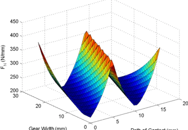
The load distribution (force per unit of length along the path of contact) disregarding elastic effects can be calculated dividing the total normal forceFn=M_r_bi_i by the total length of

the lines of contact along the path of contact.

The total length of the lines of contact along the path of contact can be calculated with the algorithm presented in Ap-pendix A. The load distribution per unit of length along the

Figure 1.Load distribution of a helical gear with an applied torque of 320 Nm.

path of contact can then be calculated according to Eq. (8). An example of the load distribution in a helical gear is pre-sented (Fig. 1).

FN(x, y)= Fbn

L(x, y) (8)

The gear loss factor can now be calculated according to Eq. (9) proposed by Wimmer (2006)

H_Vnum= 1

pb b

Z

0 E

Z

A

FN(x, y) Fb

·Vg(x, y)

Vb

dxdy. (9)

To solve Eqs. (8) and (9) the total length of contacting lines should be known at each point along the path of contact. To perform this task, an algorithm was developed and imple-mented (Appendix A).

3 Average coefficient of friction

Several authors (Ohlendorf, 1958; Eiselt, 1966; Naruse et al., 1986; Michaelis, 1987; Schlenk, 1994; Doleschel, 2002) have introduced different formulas to calculate the average coefficient of friction between gear teeth for different gear geometries. Due to the complexity of the problem, these equations are usually based in experimental results, and nat-urally, the results yielded by these models vary for the same operating conditions. In this work, instead of calculating the coefficient of friction yielded by these formulations, a value is calculated from the experimental procedure used in a pre-vious work (Fernandes et al., 2013) and then compared to the models.

Assuming thatPV Z0,PV LandPV D are correctly

(3)

T

r

a

n

s

fer

2

H5

0

1

T

r

a

n

s

fe

r

1

C4

0

m=8 m=

1

0

H95

1

0 0.1 0.2 0.3 0.4 0.5 0.6 0.7

0.4 0.6 0.8 1 1.2 1.4 1.6 1.8 2

Hv

k₀

Buckingham Ohlendorf Winter Velex Kisssoft Author

Figure 2.Gear loss factor comparisson with different formulas.

and load independent gear losses were discussed in previous works of Fernandes et al. (2013, 2015).

P_{V ZP}exp =P_Vexp−(PV Z0+PV L+PV D) (10)

Considering the power loss generated by the gears in the gearbox (Eq. 10) an average coefficient of friction (µexp_mZ) can be calculated. It can be calculated according to different ap-proaches:

1. From Ohlendof’s approach (Eq. 11).

µexp_mZ= P

exp V ZP

PIN·H_Vi

(11)

H_Vi is the gear loss factor which can assume various forms, depending on the formulation that is used. Four HV were defined according to Eq. (2) H_VOhl, Eq. (9)

H_Vnum, Eq. 3H_VNie, Eq. 4H_VBuc.

2. Considering the average power loss generated between gear teeth along the path of contact according to Velex and Ville (2009),µexp_mZcan be obtained solving Eq. (12) to findµexp_mZ.

PV ZP =PIN·µexp_mZ·(1+u)· π z1·cosβb

·ǫα·3 µexpmZ

(12)

The coefficient of friction extracted from the gear mesh power loss obtained with Eq. (10) will be dependent of the formulation that is used to calculate the gear loss factor. In order to decide which gear loss factor formulation is better suited for the authors study, this factor was calculated for seven different gear geometries, in which, spur, helical and low loss gears are included (Table 1) (Fernandes et al., 2015).

The gear loss factor was also calculated based on the results obtained with the commercial softwareKissSoft which ac-counts for elastic effects.

Figure 2 shows the comparison between the different gear geometries as a function of thek0 (Eq. 5) parameter. There

are clearly two groups of results that diverge at a certain point. A deviation is found in the solutions proposed by Buckingham (1949), Niemann and Winter (1989) and Velex and Ville (2009) because Eq. (5) is expected to yield values between 0 and 0.5. which means that it is not suitable for gears with profile shift.

The H501 and H951 geometries were previously tested for power loss in an FZG test rig (Fernandes et al., 2015). The results presented were collected for FZG load stages with a lever arm of 0.35 m, i.e. K5=105, K7=199 and K9=323 Nm applied on wheel. Changing from H501 to H951 resulted in a dramatic power loss reduction (Fig. 3), which was attributed to the H951 gear geometry (everything but the gear geometry was kept the same). These experimen-tal results suggest that the gear loss factor of the H951 must be lower than that of the H501. The trends shown by the gear loss factors obtained withKissSoft, the author’s method and Ohlendorf are in agreement with the experimental observa-tions of Fernandes et al. (2015). The gear loss factors ob-tained with Eq. (9) are close to those obob-tained with the ones derived from theKissSoftcomputations. Aiming for simplic-ity and fast computing the gear loss factor was calculated using Eq. (9).

Following Fig. 2 it becomes clear that Buckingham, Velex and Winter’s approaches are not suitable for all gear geome-tries and can only be applied over a limited range of thek0

(4)

Table 1.Geometrical parameters of the gears.

Gears Parameters

z m a α β b xz da ǫα ǫβ Ra

[/] [mm] [mm] [◦] [◦] [mm] [/] [mm] [/] [/] [µm]

C40 Pinion 16 4.5 91.5 20 0 40 +0.1817 82.64 1.44 0 0.7

Gear 24 +0.1715 115.54

H501 Pinion 20 3.5 91.5 20 15 23 +0.1381 80.37 1.45 0.54 0.3

Gear 30 +0.1319 116.57

H951 Pinion 38 1.75 91.5 20 15 23 +1.6915 76.23 0.93 1.08 0.3

Gear 57 +2.0003 111.73

Transfer 1 Pinion 32 3.5 105.0 20 20 35 +0.3810 128.45 1.32 1.09 0.4

Gear 23 +0.4150 95.17

Transfer 2 Pinion 28 4 95.0 20 20 33.5 −0.2400 125.22 1.49 0.91 0.4

Gear 17 +0.0510 80.73

m=8 Pinion 17 8 355 20 9 124 +0.4965 160.74 1.40 0.77 –

Gear 69 +0.3985 580.36

m=10 Pinion 19 10 500 20 9 175 +0.6500 222.65 1.32 0.87 –

Gear 77 +0.8877 814.63

0.0 1.0 2.0 3.0 4.0 5.0

K1 K5 K7 K9 K1 K5 K7 K9 K1 K5 K7 K9

200 400 1200

TL

[N.m]

Rotational speed [rpm]

C 40 H 501 H 951

Figure 3.Torque loss for different gear geometries lubricated with a mineral wind turbine gear oil (Fernandes et al., 2015).

4 Validation with experimental results

In order to validate the gear loss factor that was proposed, Schlenk’s (Schlenk, 1994) coefficient of friction was used (Eq. 13). The lubricant parameter (XL) was previously

de-termined with a spur gear geometry (C40) for different wind turbine gear oil formulations (Fernandes et al., 2013). Alter-natively, experimental results obtained with H501 and H951 gear geometries were presented in Fig. 3 (Fernandes et al., 2015). The gear loss factors calculated according to different approaches for the C40, H501 and H951 gear geometries are presented in Table 2.

Table 2. Gear loss factor calculated according to different ap-proaches.

HV C 40 H 501 H 951

Ohlendorf 0.1959 0.1639 0.0739 Author 0.1959 0.1873 0.0684 KissSoft 0.2039 0.2011 0.0882

µSchlenk_mZ =0.048·

Fbt/b ν6C·ρredC

0.2

·η−0.05·Ra0.25·XL (13)

In Fig. 4 the absolute error of the power loss model pre-diction using the KissSoft, Ohlendorf and Author gear loss factors is presented. The results suggest that the gear loss fac-tor presented by the authors in Eq. (9), considering the rigid load distribution, present a much lower absolute error for the prediction of a mineral wind turbine gear oil power loss for with helical gears, previously published by Fernandes et al. (2015).

Schlenk’s Equation should be valid for both helical and spur gear geometries, also H_VOhl is mostly valid for spur gears. This means that using the lubricant parameterXL

(5)

-15 -10 -5 0 5 10 15

K5 K7 K9 K5 K7 K9 K5 K7 K9

200 400 1200

er

ror

[%]

Author KissSoft Ohlendorf

(a) H501

-15 -10 -5 0 5 10 15

K5 K7 K9 K5 K7 K9 K5 K7 K9

200 400 1200

er

ror

[%]

Author KissSoft Ohlendorf

(b) H951

Figure 4.Correlation between the experimental power loss mea-sured and the predicted with Author, Ohlendorf or KissSoft gear loss factors.

5 Conclusions

In this work several gear loss factors were compared. The gear loss factor results were indirectly compared with exper-imental gear power loss measurements in order to assess the validity of each one of the formulations.

An alternative formulation based on the numerical integra-tion of the rigid load distribuintegra-tion is suggested. The method presented by the authors to solve the gear loss factor formula proposed by Wimmer (2006) disregards the elastic effects of the gears but proved to be reliable to predict the average power loss of helical and spur gears as proven with experi-mental results.

The results suggest that the classical formulas are accurate only in very specific scenarios. The comparison with the ex-perimental results indicates that the approach suggested by the authors works quite well.

(6)

Appendix A: Load distribution along the path of contact

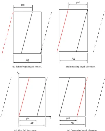
Before enter the contact zone of a gear, or the path of contact which value is given by Eq. (A1), a teeth contact line has the representation of Fig. A1a.

AE=ǫα·pbt (A1)

When the contact starts, the length of the contacting line increases proportionally to the coordinate of the path of con-tact, represented by the first condition of Eq. (A2) (Fig. A1a and b). The contact then continues to increase up to the sit-uation of a full line of contact, that occur at the coordinate x=ǫβ·pbt=b·tanβbup to the end of contact atx=ǫα·pbt

which is given by second condition of Eq. (A2) (Fig. A1c). Then, the teeth start to go out from the contact and the line length starts to decrease as shown in the third condition of Eq. (A2) and Fig. A1d.

l(x)=

             x

sinβb 0< x < ǫβ·pbt

b

cosβb ǫβ·pbt< x < ǫα·pbt

b

cosβb−

x−ǫα·pbt

sinβb ǫα·pbt< x < ǫα+ǫβ

·pbt

(A2)

Equation (A2) previously presented is valid for the length of a single line along the path of contact. The other teeth have the same behaviour of the single line yet presented but at the distance of a transverse pitch (pbt), which is the distance

between the teeth along the path of contact as represented in Fig. A1.

The same equations deduced for a single line can be used, but the coordinates should be transformed according to Eq. (A3). The value iof the Eq. (A3) is calculated with Eq. (A4) that represents the lines screened from the single line with value i=0, from behind and behead in integer steps.

x∗(x)=x+i·pbt (A3)

i= −ceil ǫα+ǫβ:1:ceil ǫα+ǫβ (A4)

Ceil is a function that rounds the value for the highest close integer.

It is also possible to do a 3-D representation of the line length as function of x andy. To do that, they coordinate representing the tooth width that changes from 0 up to b. Since the tooth line of contact of a helical gear has a helix angle they coordinate is function of thexcoordinate which can be expressed with Eq. (A5).

x₍∗_x,y₎=x+i·pbt+ytan (βb) (A5)

Applying the coordinate transformation of Eq. (A5) and the formulas of Eq. (A2), the line length of each tooth screened from the teethiis presented in Eq. (A6).

(a) Before beginning of contact. (b) Increasing length of contact.

x y

(c) After full line contact. (d) Decreasing length of contact.

Figure A1.Evolution of a single line along the path of contact.

li(x, y)=                x∗

sinβb 0< x

∗_{< ǫ}

β·pbt

b

cosβb ǫβ·pbt< x

∗_{< ǫ}

α·pbt

b

cosβb−

x∗₋_ǫ_α·_p

bt

sinβb ǫα·pbt< x

∗_{< ǫ}

α+ǫβ

·pbt

(A6)

The formulation presented is valid for gears with a contact ratioǫα> ǫβ.

For the case that one complete line is not in contact, the cycle of meshing is slightly different and the path of contact is smaller than the transverse pitch. In such cases usually the overlap contact ratio isǫβ> ǫα.

The equation is slightly different from that presented be-fore because the domains change in a different way as pre-sented in Eq. (A7).

li(x, y)=                x∗

sinβb 0< x

∗_{< ǫ}

α·pbt

ǫα·pbt

sinβb ǫα·pbt< x

∗_{< ǫ}

β·pbt

ǫα·pbt sinβb −

x∗₋_ǫ_β·_p

bt

sinβb ǫβ·pbt< x

∗_{< ǫ}

α+ǫβ

·pbt

(A7)

(7)

L(x, y)=

ceil(ǫα+ǫβ) X

−ceil(ǫα+ǫβ)

li(x, y) (A8)

Stepwise functions

The algorithm previously presented is based on the identifi-cation of different domains in the meshing cycle of helical gears. However, the different domains can be combined us-ing stepwise functions like Heaviside (Eq. A9) or hyperbolic tangent (Eq. A10).

ξ = 1

1+e−2k(x−a) (A9)

ξ =1

2·(tanh(k·(x−a))+1) (A10)

The coordinateais the point when the step is desired. Using the hyperbolic tangent equation, the three domains can be expressed in Eq. (A11) for the beginning of con-tact (a=0), Eq. (A12) for a complete line (a=ǫβ·pbt) and

Eq. (A13) for a line going out from the contact (a=ǫα·pbt).

The constant k changes the precision of the algorithm. For the case it was consideredk=1000.

ξ1=

1

2· tanh(k·x)−tanh k· x− ǫα+ǫβ

·pbt

(A11)

ξ2=

1

2· tanh k· x−ǫβ·pbt

+1 (A12)

ξ3=

1

2·(tanh (k·(x−ǫα·pbt))+1) (A13)

For each single line the length along the path of contact is given by Eq. (A14).

l(x)= 1

sinβb

·ξ1· x−ξ2· x−ǫβ·pbt

−ξ3·(x−ǫα·pbt)) (A14)

For spur gears the length for each line is given by Eq. (A15).

l(x)=b·ξ1 (A15)

For the lines screened from the one considered the length is computed with Eq. (A3) previously explained which re-sults in Eq. (A16).

li(x, y)=l

x₍∗_x,y₎ (A16)

The total sum of lines is then given by Eq. (A8).

Using such type of function or other stepwise function is great to get a continuous function. However, the computa-tional time can increase due to the expense of computing the step function. The algorithm with step function works for all the type of gear geometries and the transverse and overlap contact ratios (ǫαandǫβ) do not need to follow any rule.

Table A1.Notation and units.

a Centre distance,[mm] AE Path of contact,[mm]

b Face width,[mm]

da Addendum diameter,[mm]

HV Gear loss factor from,[–]

Fb Tooth normal force on transverse plane,[N]

F_bn Tooth normal force,[N]

FN(x, y) Normal force per length,[N mm−1]

k₀ Gear geometry factor ,[–]

l(x) Length of a single line of contact,[mm]

L(x,y) Sum of the lengths of the lines of contact,[mm]

m Module,[mm]

n Rotational speed,[rpm]

Mi Torque in geari,[Nm]

pb Base pitch,[mm]

p_bt Transverse base pitch,[mm]

PIN Input power,[W]

PV Total power loss,[W]

PV D Seals power loss,[W]

PV L Rolling bearing power loss,[W]

PV Z0 Gears no-load loss,[W]

PV ZP Gears load loss,[W]

rai Tip radius,[m]

rbi Base radius of geari,[mm]

rpi Pitch radius of geari,[mm] Ra Average roughness,[µm]

u Gear ratio,[–]

Vg(x,y) Sliding velocity,[m s−1]

Vb Base cylinder transverse tangential speed,[m s−1]

v6C Sum velocity at pitch point,[m s−1]

xz Profile shift coefficient,[–]

x Coordinate along the tooth path of contact,[mm]

XL Lubricant parameter,[–]

y Coordinate along the tooth width,[mm]

zi Number of teeth of geari,[–]

α Pressure angle,[rad]

αt Transverse pressure angle,[rad]

β Helix angle,[rad]

βb Base helix angle,[rad]

ǫ₁ Addendum contact ratio,[–]

ǫ2 Deddendum contact ratio,[–]

ǫα Transverse contact ratio,[–]

ǫβ Overlap ratio,[–]

3(µ) Efficiency parameter,[–]

η Dynamic viscosity,[mPa s−1]

µmZ Average coefficient of friction,[–]

ρ Efficiency of a gear pair,[–]

ρredC Equivalent contact radius at pitch point,[mm]

(8)

Acknowledgements. The authors gratefully acknowledge the funding supported by:

– National Funds through Fundação para a Ciência e a Tecnolo-gia (FCT), under the project EXCL/SEM-PRO/0103/2012;

– COMPETE and National Funds through Fundação para a Ciência e a Tecnologia (FCT), under the project Incen-tivo/EME/LA0022/2014;

– Quadro de Referência Estratégico Nacional (QREN), through Fundo Europeu de Desenvolvimento Regional (FEDER), un-der the project NORTE-07-0124-FEDER-000009 – Applied Mechanics and Product Development;

without whom this work would not be possible.

Edited by: P. Flores

Reviewed by: two anonymous referees

References

Buckingham, E.: Analytical mechanics of gears, Dover Books for Engineers, republished by Dover Publication, 1963, McGraw-Hill Book Co., New York, 1949.

Doleschel, A.: Wirkungsgradtest, Vergleichende Beurteilung des Einflusses von Schmierstoffen auf den Wirkungsgrad bei Zahnradgetrieben, FVA Forschungsvorhaben Nr. 345, FVA Forschungsheft Nr. 664, FVA, Germany, 2002.

Eiselt, H.: Beitrag zur experimentellen und rechnerischen Bestim-mung der Fresstragfähigkeit von Zahnradgetrieben unter Berück-sichtigung der Zahnflankenreibung, PhD thesis, Dissertation TH Dresden, Dresden, 1966.

Fernandes, C. M., Martins, R. C., and Seabra, J. H.: Torque loss of type C40 FZG gears lubricated with wind turbine gear oils, Tribol. Int., 70, 83–93, doi:10.1016/j.triboint.2013.10.003, 2013. Fernandes, C. M., Marques, P. M., Martins, R. C., and Seabra, J. H.: Gearbox power loss, Part II: Friction losses in gears, Tribol. Int., 88, 309–316, doi:10.1016/j.triboint.2014.12.004, 2015. Höhn, B.-R., Michaelis, K., and Hinterstoißer, M.: Optimization of

gearbox efficiency, goriva i maziva, 48, 462–480, 2009. Kragelsky, I., Dobychin, M., and Kombalov, V.: Friction and Wear:

Calculation Methods, Pergamon Press, Oxford, 1982.

Michaelis, K.: Die Integraltemperatur zur Beurteilung der Fresstragfähigkeit von Stirnrädern, PhD thesis, Dissertation TU München, München, 1987.

Naruse, C., Haizuka, S., Nemoto, R., and Kurokawa, K.: Studies on Frictional Loss, Temperature Rise and Limiting Load for Scor-ing of Spur Gear, Bull. Jpn. Soc. Mech. Eng., 29, 600–608, doi:10.1299/jsme1958.29.600, 1986.

Niemann, G. and Winter, H.: Maschinenelemente: Band 2: Getriebe allgemein, Zahnradgetriebe – Grundlagen, Stirnradgetriebe, Maschinenelemente/Gustav Niemann, Springer, München, Ger-many, 1989.

Ohlendorf, H.: Verlustleistung und Erwärmung von Stirnrädern, PhD thesis, Dissertation TU München, München, 1958. Schlenk, L.: Unterscuchungen zur Fresstragfähigkeit von

Grozahn-rädern, PhD thesis, Dissertation TU München, München, 1994. SKF: SKF General Catalogue 6000 EN, SKF, November 2005. Velex, P. and Ville, F.: An analytical approach to tooth friction

losses in spur and helical gears-influence of profile modifica-tions, J. Mech. Design, 131, 1–10, 2009.