3D Stress intensity factor and T-stresses (T11 and T33) formulations for a Compact Tension specimen

(1)

S. K. Kudari et alii, Frattura ed Integrità Strutturale, 39 (2017) 216-225; DOI: 10.3221/IGF-ESIS.39.21

216

3D Stress intensity factor and T-stresses (T

11

and T

33

)

formulations for a Compact Tension specimen

S. K. Kudari

Department of Mechanical Engineering, CVR College of Engineering, Hyderabad, India

s.kudari@rediffmail.com

K. G. Kodancha

Research Centre, Department of Mechanical Engineering, BVB College of Engineering & Technology, Hubli, India krishnaraja@bvb.edu

ABSTRACT. The paper describes test specimen thickness effect on stress intensity factor (KI), and T-stresses stresses (T11 and T33) for a Compact

Tension specimen. Formulations to estimate 3D KI, T11 and T33 stresses are

proposed based on extensive 3D Finite element analyses. These formulations help to estimate magnitudes of 3D KI and T11 and T33 which are helpful to

quantify in-plane and out-of- plane constraint effect of the crack tip. The proposed formulations are validated with the similar results available in literature and found to be within acceptable error.

KEYWORDS. Constraint effects; 3D Finite element analysis; Stress intensity factor; T-stress; CT Specimen.

Citation: Kudari, S. K., Kodancha, K. G., 3D Stress intensity factor and T-stresses (T11

and T33) formulations for a Compact Tension

specimen, Frattura ed Integrità Strutturale, 39 (2017) 216-225.

Received: 25.09.2016

Accepted: 31.10.2016

Published: 01.01.2017

Copyright: © 2017 This is an open access article under the terms of the CC-BY 4.0, which permits unrestricted use, distribution, and reproduction in any medium, provided the original author and source are credited.

INTRODUCTION

tress tri-axiality at the crack-tip can alter crack-tip constraint and fracture toughness values of a material. This is the reason transferability of fracture toughness data estimated using laboratory test specimens to a full-scale cracked structure is an important issue in structural integrity assessment of engineering materials. In LEFM zero non-singular terms in the series expansion of three-dimensional stress field [1] referred as T-stresses (T11 and T33) can alter the

crack-tip stress tri-axiality and are considered as constraint parameters [2]. T11 (the second term of William’s extension

acting parallel to the crack plane) plays an important role on the in-plane constraint effect. The thickness at the crack tip contributes to the out-of-plane constraint, T33 (the second term of William’s extension acting along the thickness). To

transfer fracture toughness data under different constraints, both in-plane and out-of-plane constraint effect should be considered for the specimens.

(2)

217

Several researchers [3-13]have shown that the specimen thickness has major effect on the magnitude of stress intensity factor and T stresses. Kwon and Sun [7] have presented 3D FE analyses, to investigate the stress fields near the crack-tip and suggested a simple technique to determine 3D KI at the mid-plane by knowing 2D KI and Poisson’s ratio () of the

material using the Eq. (1):

D

D K K

3

2 2

1

1 



 (1)

For quantifications of in-plane and out-of- plane constraint issues, magnitudes of T11 and T33 stresses are to be computed.

But simple formulations such as Eq. (1) to estimate 3D KI, are not available to compute constraint parameters, T11 and

T33 stresses. Usually they are obtained by complex 3D numerical methods.

The aim of this investigation is to study the variation of KI, T11 and T33 along the crack-front considering a CT specimen

geometry having varied thickness, B, crack length to width ratio (a/W) and applied stress, , using 3D elastic FE analysis. Based on the present finite element results an effort is made to formulate approximate analytical equations to estimate the magnitudes of maximum 3D KI, T11 and T33 for a CT specimen. The proposed analytical formulations can be used to

estimate the maximum 3D KI, T11 and T33 for the CT specimen, which are helpful in quantifying in-plane and

out-of-plane constraint issues in fracture. By means of numerical analyses, it is shown that specimen thickness and crack length play an important role on the constraint effects.

Figure 1: The geometry of the CT specimen used in the analysis (W=20 mm).

FINITE ELEMENT ANALYSIS

ommercial FE software ABAQUS 6.5 [14] is used for the 3D FEA. The dimensions of CT specimen have been chosen according to ASTM standard E1820 [15] and the specimen geometry is shown in the Fig.1. One-half of the specimen geometry is modeled due to specimen symmetry. Twenty noded quadratic brick elements available in the ABAQUS are used to discretize the analysis domain. This kind of elements was used in the earlier works [8, 9] available in the literature. Initially, three-dimensional FE analyses on CT specimens were made by varying number of layers in thickness direction (each layer is of element thickness). It is observed that the variation in results of KI is

insignificant for 8-14 layers. Consequently, in the present analyses 11 layers along the thickness direction were chosen as it gives ten numbers of elements along the thickness direction to extract the KI and T-stress. Due to half symmetry, the

symmetrical boundary conditions have been imposed (ux2=0) along the ligament of the model. Load is applied on

approximately 1/3rd_{portion nodes of the loading-hole circle perpendicular to the ligament. To keep the loading in}

perfectly Mode-I condition corresponding nodes are arrested except x2-direction. A typical mesh used in the analyses

along with boundary conditions is shown in Fig.2. The magnitudes of KI and T-stresses have been extracted by using

ABAQUS post processor. The details of extraction of stress 3D stress intensity factor (KI) and T-stresses are discussed

elsewhere [11,12,16,17].The variation of KI and T-stresses along the crack-front has been studied for different specimen

thickness (B/W=0.1-1.0) and crack length to width ratio (a/W=0.45-0.70). In this work the magnitude of applied stress,

, for the CT specimen is computed using the relation [18]:

(3)

218

P W a B W 2

2 (2 )

( )

   (2)

where, P is applied load, W is width of the specimen, a is crack length. In these finite element calculations, the material behaviour has been considered to be linear elastic pertaining to an interstitial free (IF) steel possessing yield stress

y=155MPa, elastic modulus of 197 GPa, Poisson’s ratio=0.30.

Figure 2: 3D CT Specimen mesh along with boundary conditions for a/W=0.50: a) B/W=0.1; b) B/W=1.

Figure 3: Effect of a/W on normalized stress intensity factor, KI /(a)1/2 along crack-front (x3) for B=10mm.

RESULTS AND DISCUSSION

Stress Intensity Factor (KI)

typical variation of normalized stress intensity factor (KI/(a)1/2) and the distance along the crack front

(specimen thickness direction, x3) for specimens having various a/W is shown in Fig.3. The nature of variation of

normalized stress intensity factor shown in Fig.3 is in good agreement with the similar results [7,19]. The

(4)

219

magnitudes of 3D maximum stress intensity factors (at the center of the specimen) are compared with the analytical 2D value computed by Eq. (3).

I

K Y a (3)

Typically, such comparison for a specimen with a/W=0.65 is shown in Fig.3. It is estimated that magnitude of 2D KI is

about 10% lower than 3D KI.

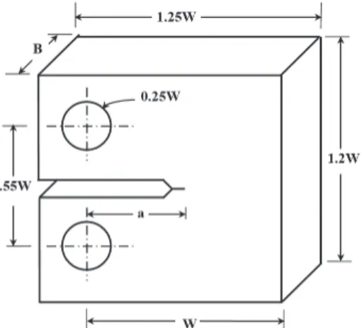
It is well known that variation of stress intensity factor against  

 

a 1/2 for various specimen thickness (B) is linear,

slopes of KI-max vs.  

 

a 1/2 obtained for various a/W are plotted in Fig 4. As the relation between KI-max/ 

 

a 1/2and

a/W (Fig.4) is nonlinear, the data is fit with a suitable polynomial. In such exercise, it is found that a polynomial equation of third order fits the 3D FEA results with least error (Regression co-efficient=0.998). This polynomial fit (Eq. (4)) is superimposed on the 3D FEA results plotted in Fig.4 and shows an excellent agreement. From this third order polynomial fit, the relation between KI-max, a/W and  can be expressed as:

KI a a a

W W W

a

2 3

max _{4.48287 14.99985} _20.44016 _3.85185

 

 _ _  _   _  

     

      (4)

Let,

a a a

C

W W W

2 3

1 4.48287 14.99985 20.44016 3.85185

     

  _ _ _ _  _ _

      (5)

Figure 4: Variation of slopes, KI-max/  a 1/2vs. a/W.

The Eq. (4) reduces to:

I

K __maxC₁ a (6)

Eq. (6) is similar to Eq. (3) and the constant C1 shown in Eq. (5) is similar to the geometric factor, Y as used in Eq. (3).

Hence, C1 in this work is referred as 3D geometric factor. Eq. (6) can be used to estimate magnitudes of KI-max for the

CT specimen. To validate the proposed formulation given in Eq. (6), the computed values of KI-max using Eq.(6) for

(5)

220

present 3D FEA for a/W 0.45 to 0.70 (entire range of study). The values of KI-max estimated from the Eq.(1) [7] are found

to in good agreement with the present results for specimens with a/W 0.45 to 0.65, but for a specimen having a/W>0.65 the Eq.(1) [7] is showing higher error. The error analysis between the results obtained by present 3D FEA and the Eq.(6) is conducted. The maximum percentage of error estimated in use of Eq.(6) for B=2 to 20mm and a/W=0.45 to 0.70 is < 2.95 %.

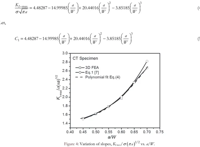
Figure 5: A typical variation of T11/along the crack-front for various B and a/W=0.50.

T11-stress

The magnitudes of T11 are extracted from 3D FE analysis for varied , B and a/W. A typical variation of T11 along the

crack-front for various B, a/W=0.50 and  =86.8 MPa is shown in Fig.5. This figure shows that the variation of T11 along

the crack-front (x3) depends on the specimen thickness. It is observed that the magnitude of T11 is maximum at the centre

of the specimen than on the surface. However, for the specimen thickness, B<6mm the maximum value of T11 is found to

be just below the surface. It is seen from Fig.5 that for specimen with higher thickness, the magnitude of T11 decreases for

a short distance from the specimen surface and again increases at the centre of the specimen thickness. Similar kind of variation was observed in the work of Pavel et al. [20]. To study the effect of a/W, a typical variation of T11/ for various

a/W, B=10mm and  =86.8 MPa is plotted in Fig.6. The figure illustrates that T11 depends on the specimen a/W, and it is

observed to be maximum for higher a/W. The results in Fig.5-6 indicate that the in-plane constraint parameter, T11, is not

a unique value (as obtained in 2D analysis) for a specimen thickness, but it varies along the thickness and it is maximum at the centre.

The variation of T11 at the center (T11-max) vs. normalized KI (KI-max/(πB)1/2) for various specimen thicknesses is studied.

A typical plot of T11-max against KI-max/(πB)1/2 for various a/W and B=10 mm is shown in Fig.7. It is seen from the Fig.7

that the variation of T11-max vs. KI-max/(πB)1/2 is linear and is independent of a/W. The slopes of T11-max vs. KI-max/(πB)1/2

are computed for various a/W by fitting a straight-line equation to all the results shown in Fig.7. The estimated slopes T 11-max/(KI-max/(πB)1/2) are plotted against normalized thickness (B/W) for various a/W in Fig. 8. This plot indicates that, the

nature of variation of slopes T11max/ (KI-max/(πB)1/2) against B/W is nonlinear and is almost independent of a/W. The

result plotted in Fig.8 is used to obtain a relationship between T11-max and KI-max. As there is a small difference is observed

in the results presented in Fig.8 for various a/W, the average slope of all a/W for particular B/W is used. The average results are fit by a polynomial equation of third order (Regression Co-efficient=0.994), which give a best fit to all the data. From this third order polynomial fit, the relation between T11-max and KI-max is obtained and can be expressed as:

I

T B B B

K W W W

B

2 3

11 max

max

0.1477 0.93746 0.87183 0.35186

  

     

  _ _ _ _  _ _

       

 

 

(6)

221 Figure 6: A typical variation of T11/ along the crack-front for

various a/W and B=10mm.

Figure 7: Variation of T11-max against KI-max/πB1/2 for various a/W and B=10 mm.

Figure 8: Variation of slopes T11-max/(KI-max/(πB)1/2 against B/W for various a/W.

Let,

B B B

C

W W W

2 3

2 0.1477 0.93746  0.87183  0.35186 

      (8)

The Eq. (7) reduces to:

I K

T C

B

max 11- max 2 _

 

 _ _

  (9)

(7)

222

a

T C C

B

11 max 1. 2.  

 

 

 _ _

  (10)

a

T C C

B

11- max 1. 2. (11)

where, constant C1 and C2 are referred in this work as 3D geometric factors. The values of C1 for various a/W and C2 for

various B/W for the CT specimen are tabulated in Tab.1 and Tab.2 respectively.

a/W 0.45 0.50 0.55 0.60 0.65 0.70

C1 1.5211 1.6115 1.7753 2.0094 2.3111 2.6775

Table 1: Values of C1 computed from Eq.(5).

B/W 0.1 0.2 0.3 0.4 0.5 0.6 0.7 0.8 0.9 1.0

C2 0.2331 0.3031 0.3600 0.4057 0.4425 0.4723 0.4974 0.5199 0.5417 0.5652

Table 2: Values of C2 computed from Eq.(8).

The above Eq.(11) can be used to estimate T11-max for the CT specimen for a given specimen dimensions and applied load, . A typical plot of T11-max computed from Eq.(11) is superimposed (Red curve) on 3D FEA results shown in Fig. 8. This

plot shows a good agreement with the results estimated by Eq.(11) and 3D FEA. An error analysis is carried out between the estimated values from Eq.(11) and the present 3D FEA results. The maximum percentage of error in use of Eq.(11) for various B, a/W and  used in this study is foundto be < 5.1%. The proposed analytical Eq.(11) is a simple method to compute T11-max for the CT specimen geometry.

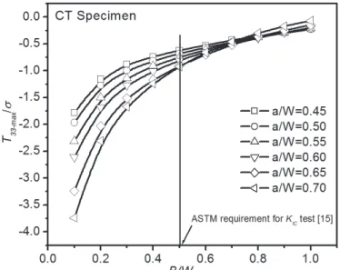
Figure 9: Variation of T33/ against B/W for various a/W.

T33-stress

The magnitudes of T33 are estimated using Eq.(12) by substituting the extracted 33 (strain) from ABAQUS post processor

and T11 for varied , B and a/W.

(8)

223

The variation of T33-max/ against B/W for various a/W is shown in Fig.9. This figure indicates that, T33 strongly depend

on B/W. It is observed that the magnitude of T33 is negative for all cases that were considered in this analysis, and

approached to zero as B/W increased to 1. For B/W=0.5, ASTM requirement for KIC test specimen [15], it is seen that

T33 / is negative indicating loss of out-of-plane constraint. T33 also showed dependence on a/W, for B/W<0.7, T33 is

found to be maximum for thinner specimens (B/W=0.1) with higher a/W =0.7. As T33 strongly depends on the specimen

thickness, it is not possible to get a simple relation between T33 and specimen geometry as obtained in case of KI and T11.

To obtain expressions between T33,specimen geometry and the applied load, the results in Fig.9 are given a polynomial fit

to suit the 3D FEA results. In this exercise, it is found that the 5th_{order polynomial fits the data with least error. A typical}

equation for estimation of T33–max is given by Eq. (13). The equations for the 3D geometric factors (C3) to compute T33-max

for various a/W obtained by fitting 5th_{order polynomial are tabulated in Tab.3.}

T_{33- max} C₃ (13)

The computed values of C3 for various a/W are given in Tab.4. The maximum percentage of error in the use of equations

given in Tab.3 for various B, a/W and  is found to be < 7.8%.

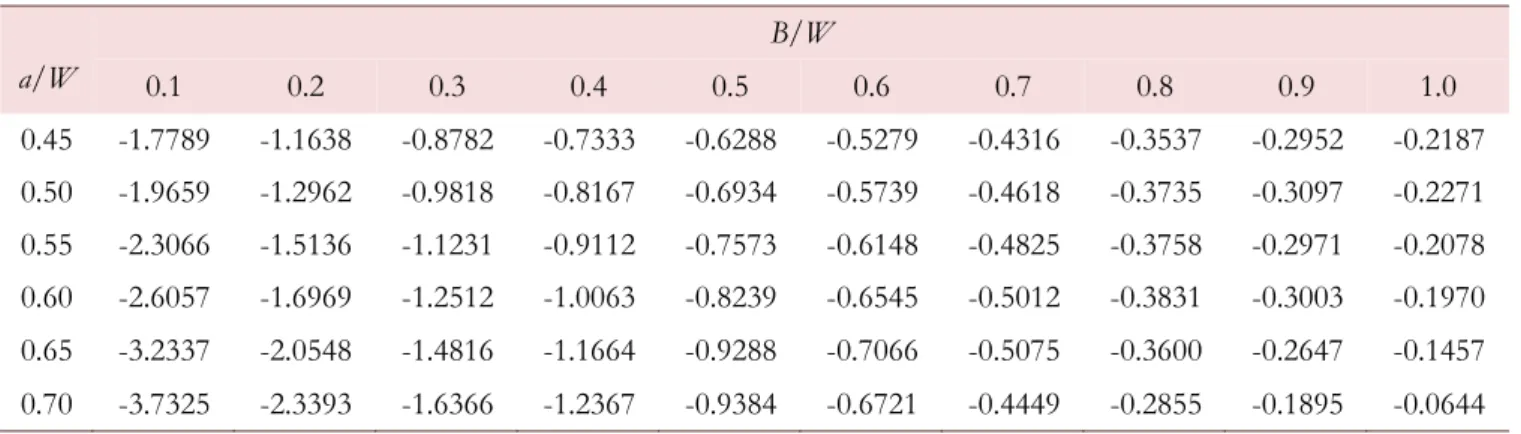
Table 3: Polynomial equations for T33.

a/W

B/W

0.1 0.2 0.3 0.4 0.5 0.6 0.7 0.8 0.9 1.0

0.45 -1.7789 -1.1638 -0.8782 -0.7333 -0.6288 -0.5279 -0.4316 -0.3537 -0.2952 -0.2187

0.50 -1.9659 -1.2962 -0.9818 -0.8167 -0.6934 -0.5739 -0.4618 -0.3735 -0.3097 -0.2271

0.55 -2.3066 -1.5136 -1.1231 -0.9112 -0.7573 -0.6148 -0.4825 -0.3758 -0.2971 -0.2078

0.60 -2.6057 -1.6969 -1.2512 -1.0063 -0.8239 -0.6545 -0.5012 -0.3831 -0.3003 -0.1970

0.65 -3.2337 -2.0548 -1.4816 -1.1664 -0.9288 -0.7066 -0.5075 -0.3600 -0.2647 -0.1457

0.70 -3.7325 -2.3393 -1.6366 -1.2367 -0.9384 -0.6721 -0.4449 -0.2855 -0.1895 -0.0644

Table 4: Values of C3 computed from formulations given in Tab.3.

a/W Polynomial Equations

0.45 T B B B B B

W W W W W

2 3 4 5

33 max _{3.02667 16.98748} _53.07517 _86.44814 _68.70629 _21.15385

                

0.50 T B B B B B

W W W W W

2 3 4 5

33 max _{3.32333 18.49597} _58.0134 _95.41084 _76.51515 _23.71795 

         

   _ _ _ _  _ _  _ _  _ _

         

0.55 T B B B B B

W W W W W

2 3 4 5

33 max _{3.858 20.88005} _62.97348 _100.77273 _79.1317 _24.10256

                

0.60 T B B B B B

W W W W W

2 3 4 5

33 max _{4.40067 24.26372} _74.31294 _121.11772 _96.8648 ₃₀                 

0.65 T B B B B B

W W W W W

2 3 4 5

33 max _{5.582 31.84602} _98.58275 _162.16142 _130.62937 _40.64103                 

0.70 T B B B B B

W W W W W

2 3 4 5

33 max _{6.44533 36.53654} _110.79021 _181.22902 _146.36364 _45.76923 

         

   _ _ _ _  _ _  _ _  _ _

(9)

224

To evaluate the worthiness of the analytical expressions to estimate KI-max, T11-max and T33-max proposed in this analysis, the

estimated magnitudes KI-max, T11-max and T33-max obtained by Eq.(6), Eq.(11) and Tab.3 are compared with the similar

results on the CT specimen presented by Toshiyuki and Tomohiro [12]. The authors [12] have given the variation of T 11-max and T33-max for the toughness value of the material (0.55% Carbon Steel) KI-max= 66 MPam1/2. Fig. 10 shows a typical

variation of estimated KI-max, T11-max and T33-max at the specimen thickness center against B/W (0.1 -1.0) obtained by

proposed analytical expressions (Eq.(6), (11) and Tab.3) for KI-max= 66 MPam1/2 and results of Toshiyuki and Tomohiro

[12]. The authors [12] have computed various parameters for B/W=0.25, 0.4 and 0.5 only. According to Fig. 10, the magnitudes of KI-max were not affected by B/W as expected and are in excellent agreement with Toshiyuki and Tomohiro

[12]. T11 showed visible dependence on B/W, though the variation was less than 20% and it is in good agreement with the

earlier reported results [12]. In summary, the in-plane parameters at the specimen thickness center showed small dependence on B, and are in excellent agreement with the earlier results [12] providing validation for the proposed Eq.(6) and (11). On the other hand, out-of-plane constraint factor, T33 showed strong dependence on B/W. T33 was found

negative and approached zero as B/W increased from 0.1 to 1. Fig. 10 shows that the nature of variation of present results of T33 (obtained by Tab.3 expressions) is in similar manner to the one presented by Toshiyuki and Tomohiro [12].

However, some difference in the magnitude of T33 between both the results for B/W=0.25-0.5 is observed. This

difference is attributed to the effect of side grooves in the CT specimen used in the work of Toshiyuki and Tomohiro [12]. The side grooves in the specimen affects the strain distribution in the out-of-plane direction and restricts the value of T33 (Ref. Eq.(12)). To study this effect, we have conducted 3D FEA on CT specimen used by Toshiyuki and Tomohiro

[12] without side groove and for the same material properties. These computed results are superimposed in Fig.10 by red colored lines for comparison. This plot show that the results (KI-max, T11-max and T33-max) for the specimen without side

groove match with the one computed by the analytical expressions (Eq.(6), (11) and Tab.3) proposed in this work. This exercise infers that the use of side grooves in a specimen controls 33 and improves the out-of-plane constraint

(Ref.Fig.10: for a/W=0.5, T33 is improved from -150 MPa to -84 MPa (44%) by using 10% side groove [12]). The Fig. 10

provides validation to the proposed analytical formulations to estimate KI-max, T11-max and T33-max.

Figure 10: A typical variation of KI-max, T11-max and T33-max against B/W obtained by proposed analytical expressions and results of Toshiyuki and Tomohiro [12].

SUMMARY

n this study, stress intensity factor and T-stress (T11 and T33) solutions for CT specimens for wide range of specimen

thickness and crack lengths were computed using 3D elastic FEA. It is observed that magnitude of T33 (Ref: Fig.(9))

is highly negative for B/W=0.1 (thin specimens), and almost zero for B/W=1 (thick specimens), indicating that the thick specimens have higher out-of-plane constraint. For B/W=0.5, ASTM requirement for KIC test [15], it is observed

(10)

225

that T33 / is negative indicating some loss of out-of-plane constraint. For the specimens with similar a/W and B/W the

loss of out-of-plane constraint (T33) is much significant than the in plane constraint (T11) (Ref. Fig.10). This infers that the

major constraint loss in a CT specimen is due to the out-of-plane effects. The out-of-plane constraint loss can be corrected to some extent by providing side grooves to a CT specimen. Using the present 3D FEA results, approximate analytical formulations are proposed to evaluate the KI-max, T11-max and T33-max by knowing only applied stress and specimen

dimensions. These formulations can be helpful in the analysis of in-plane and out-of-plane constraint issues.

REFERENCES

[1] Nakamura, T., Parks, D. M., Determination of elastic T-stress along three-dimensional crack fronts using an interaction integral, Int. J. Solids Struct., 29 (1992) 1597–1611.

[2] Betegon, C., Hancock, J. W., Two-parameter characterization of elastic–plastic crack tip fields, J Appl Mech., 58 (1991) 104–110.

[3] Kudari, S. K., Kodancha, K. G., A new formulation for estimating maximum stress intensity factor at the mid plane of a SENB specimen: Study based on 3D FEA, Frattura ed Integrità Strutturale, 29 (2014) 419-425.

[4] Nakamura, T., Parks, D. M., Three-dimensional crack front fields in a thin ductile plate, J. Mech. Phys. Solids., 38 (1990) 787–812.

[5] Nevalainen, M., Dodds, R. H., Numerical investigation of 3-D constraint effects on brittle fracture in SE(B) and C(T) specimens, Int. J. Fract., 74 (1995) 131–161.

[6] Leung, A. Y. T., Su, R.K.L., A numerical study of singular stress field of 3D cracks, Finite Elem. Anal. Design., 18 (1995) 389–401.

[7] Kwon, S. W., Sun, C.T., Characteristics of three-dimensional stress fields in plates with a through -the-thickness crack, Int. J. Fract., 104 (2000) 291-315.

[8] Jie, Q., Xin, W., Solutions of T-stresses for quarter-elliptical corner cracks in finite thickness plates subject to tension and bending, Int. J. Pres. Ves. Pip., 83 (2006) 593–606.

[9] Moreira, P. M. G. P., Pastrama, S. D., Castro, P. M.. S. T., Three-dimensional stress intensity factor calibration for a stiffened cracked plate, Engng. Fract. Mech., 76 (2009) 298–2308.

[10]Kodancha, K. G., Kudari, S. K., Variation of stress intensity factor and elastic T-stress along the crack-front in finite thickness plates. Frattura ed Integrità Strutturale, 8 (2009) 45-51.

[11]Toshiyuki, M., Tomohiro, T., Kai, L., T-stress solutions for a semi-elliptical axial surface crack in a cylinder subjected to mode-I non-uniform stress distributions, Engng. Fract. Mech., 77 (2010) 2467-2478.

[12]Toshiyuki, M., Tomohiro, T., Experimental T33-stress formulation of test specimen thickness effect on fracture

toughness in the transition temperature region, Engng. Fract. Mech., 77 (2010) 867-877.

[13]Kai, L., Toshiyuki, M., Three-dimensional T-stresses for three-point-bend specimens with large thickness Variation, Engng. Fract. Mech., 116 (2014) 197-203

[14]ABAQUS V 6.5-1. (2004) Hibbitt, Karlsson & Sorensen, Inc.

[15]American Society for Testing and Materials., Standard Test Method for Measurement of Fracture Toughness, (2015) ASTM E1820-15a.

[16]Moran, B., Shih, C. F., Crack tip and associated domain integrals from momentum and energy balance. Engng. Fract. Mech., 27 (1987) 615-642.

[17]Gosz, M., Dolbow, J., Moran, B., Domain integral formulation for stress intensity factor computation along curved three-dimensional interface cracks. Int. J Solids Struct., 35 (1998) 1763-1783.

[18]Priest, A. H., Experimental methods for fracture toughness measurement, J. Strain Analysis, 10 (1975) 225-232. [19]Fernandez, Z. D., Kalthoff, J. F., Fernandez, C. A ,Canteli, A., Grasa, J., Doblare, M. Three dimensional finite

element calculations of crack-tip plastic zones and KIC specimen size requirements, ECF-15, (2005)