Modelos dinâmicos não lineares e aplicações de quadratura gaussiana

..

- - - ＭｾＭＭＭＭＭＭＭＭＭｾＭ ｾｾ＠

..,

' " #"FUNDAÇAO

' "

GETULIO VARGAS

EPGE

Escola de Pós-Graduação em

Economia

Coordenação: Prof. Rubens Penha Cysne

Diretor de Pesquisa da EPGEIFGV

Email: rubens@fgv.br-

Ir

(021) 536-9245

"MODELOS DINÂMICOS

Ni,)

--LINEARES E APLlCAÇOES

DEQUADRATUBA

GAUSSIAl\TA"

, .

HELIOMIGON

(COPPE - UFRJ)

LOCAL

Fundação Getulio Vargas

Praia de Botafogo, 190 - 10° andar - Auditório

DATA

08/05/97 (5

a

_feira)

｟Ｎｾ＠ _ _ _ _ _ _ _ _ _ _ a _ _ _ _ _ _ _ ' " ｟ｾ＠ • _ _ _ _ _ ---4._-- ___ '" __ ｾ＠

j

•

.

i: _I

SIMULATION ANO COMPUTATION

!

Volume 25

Number 2

1996

,

' , . ' , .,.:," .

Ｌｾ＠ , ' t ' ';"1"

<:».:.;

',o

I

, 'I

J

.• -i'· f '< ..• ｾ＠ ', •• ｾ＠. " . • •.• _....:... ... ｾ＠ ••. ｟ｾ＠ ... _ •. _ • .:. '..-..'_oo.__" .• _ ' _ 1 ' .. :.:... ".'" '

-COMMUN. ｓｔａｬｬｓｔＮＭｓｾｍｕｌａ＠ .• 25(2), 369-380 (1996)

LONGITUDINAL DATA ANALYSIS OF ANIMAL GROWTH

VIA MULTIVARIATE DYNAMIC MODELS

Emanuel P. Barbosa

Institulo de Ciências Exalas - UFMG

CP 702 - 30161-970 - Belo Horizonle, MG - Drazil

e-mail: emanuel al oraculo.1cc.ufmg

Helio S. Migon

Instituto de Malemática - UFRJ

CP 68530 - 20944-970 - Rio de Janeiro, RJ - Brazil

e-mail: mad02014 at ufrj.bilnel

Key Words &t. Phrafles: Longitudinal dala; Animal growlhj

Dynamic hierarchical modelsj Biological paramclcrs.

ABSTRACT

We propose mo deIs to analyze animal growlh data wilh lhe aim of eslimating and predicting quanlities of Liological and

eco-nomical interest such as the maturing rate and asymptotic weight.

lt is also studied lhe effect of environmenlal facLors of relevant

influence in the growlh processo

The models considered in this paper are based on an extension and specialization of the dynamic hierarchical model (Gamerman " Migon, 1993) lo a non-Iinear growlh curve sdLillg, where some of the growth curve parameters are considered cxchangeable among lhe unils. The inferencc for thcse models are appruximale

conju-gale analysis Lascd on Taylor series cxpallsiulIs aliei linear Bayes

procedures.

369

COfIyrilhl O 1996 by Mareei Dckker. Inc,

ｾ＠

- - - . - -- .'-- --,-'

..

•

, I

, ｾＧ＠

f

o' i o

t:

o,' ;

.

,

.r' ,

á

.!:

I'

ＮｾＮ＠

t

,I i

ｾ＠f'

,i. ,i, ·1 t

,

t-•

F

....

.

' t

'1

..

+

-!' .

:r

lo

"

to

\ O

k

•

310

.... _{... .}

BARBOSA ANO MIGON

1. INTRODUCTION

Longitudinal data of growt h ｵｾｵ｡ｬＱｹ＠ prCRcnt non-linear hdulVior in rda

lion lo the assessmenl eondition, as for instance the time. and are oh!\crvf'd for more than one individual or experimental unit, A typir.al el\se i!\ LI.,!

study or animal growth, wherr. the ｭ｣｣ｨ｡ｮｩｾｲｮ＠ nf growth nf inciividuah;

"r

a'cerlain race are charaderi1.cd by biologieal fadors of genetic nature, aluI environmenlal fadors (sce for instancc, Filzhugh,1976),

In this paper, ｭｯ､･ｬｾ＠ are proposcd lo analy7.c growlh data of ('all.l.·

(weight ｾｲＮｲｳｵｳ＠ age, corresponding to lhe monitoring of eows of a crrLaill

race), with the aim or cstimaling and predicting quanlilies of biolop;kl\l muI

economical interesl such as maturing rate (measure of how quick lhe animal

reaches its final weighl) and asymptotic weight. The informalion cnnlailwd

in these paramelers iR imporlanl for lhe dcsign of animal improvf!rtI':lIl

programs to increase the efficiency of lhe production process, It i!\ al!\o

sludied the effect of environmenlal faetors of rclevant influence in lhe growL 11 process luch as the animal birlh season .

A

lradilional univariale modeling of lhesc dala lhrough cla!\!\if'al

growth curves surrers from lhe 50 callcd aggregalion dilemma (Blalllwrr. 1.;

George, 1991): a single curve for lhe enlire data sel ('pooled mocld') si .. for

excess or aggregalion and con5cquent los5 of information and, on ti •• ! othr.r

hand, an independenl model for cach individual can (and in fad it cl.Jr.s) presenl instabilily in lhe parameler eslimales: sueh problcm i!\ apPlf)õlcllccl through shrinkage procooures ha.o;ed on hierarr.hieal and sharr·rJ paraIJlf:lf!r models. Since the inilial prescnlation of the so callcd hicrard.i.:al IJlflflds

by Lindley k Smilh (1972) 1\.0; a ncxible Baye5ian modelling slr1lf:l 1Ifr. ror

data analysis, itR practical use has been frequent, as for inslancf', ill

Ila<:Íne-Poon (1985), BlaLLberg

k

George (1991), Lange, Carlin k Gc\fano (1992)

and many olherR .

The elass of modcl .. considercd in lhis pllper ean bc ｩｬｬｬｲＮｲＢｲ｣ｬＬｾ､＠ ;tS

a mulLivarialc cxLcnLion or lhe modds inlroduccd by Migon 1./ <:arnr.rtrll\tI

(1993) or, alLernalively, aS a nnn-linr.nr cxtf!nlion of lhe modds ｰｬｦｾｳｦｾｬｉｬｲＮ｣Ｑ＠ I,y

Barbosa k Ilarrison (1992). Thc rormer is bascd on an ｣ｸｬＨｾｮｳｩｯ＠ .. allll lipe·

cialization of lhe dyllamic hierarchical modcl (Gamerman Iv ｾｉｩｲＬｯｬｬＮ＠ 199:1)

to a growLh curve seLting, where ali lhe parameters are consider,.,J ('Xdll\lIg"-able among lhe units nf same birlh scason.

The hierarchi<:al rlynamic mndels ｰｲｯｰｯｳＨｾ｣ｩ＠ in lhili ｰ｡ｊｬｦｾｉ＠ ｡ｬＧｾ＠ "dil ... d

in Lhrce parls OI' stagCR. In lhe firsl one, a :i-paramclrr p,l'Owl" "111 \',. i"

defined for esch unil (whcrc lhc pl\rllnrclers have lhe inlcqm'lóllioll or lua

turjng ralc, growlh rador

t.t.

asymplolie wcightl, anci lilochasli,' ,'ollsllailll"

(strucLural information) are irnpo!lcd on ｬｨｃｒＨｾ＠ paralllel('rs i .. t.I ... s."ou"

sLagc accorrling lo lhrN! ,lirf(!rcnl ｨｹｰＨＩｬｬｲ･ｾｩｳ［＠ IlIodel 1 . 1111' IlIallll'ill/: l;tI"

paramclcr ext:hallgeabh: RIIIUIIV, lhe ullils, model 2 . IlIal.lllill/'. pai,'

a, •

.!

,

•

" "

'. ' .. ',' ::. . .

". ,:'/' /'':'

Ｚｾ＾Ｚ＠

:'::: :,::', ',::,:

" , . !

" - c " I , '

ｾＮＭＭＭＭ ｾＧＮＭ

.... ' ... --- ...

ＮＮＡＮＭＭ｟ＮＭＭＮＭＮ｟Ｎｾ＠

--.

I ,

I

I

I

I

1

I

I .I

,

ANALVZING ANIMAL GROwrn DATA 371

growlh faclor exchangcablc and model 3 - all lhe paramelera exchange-aLiei lhe lhird parl of lhe model (evolulion equalion) expresses lhe dynamic cvolulion of lhe paramelers,

The inference for lhese models are approximale conjugale analyais based on 111 order Taylor Series expansions and linear Bayes procedures; lhe implemenlation or these models are made considering flal priors and some practical procedures such as: discounl faclors for lhe dynamic evolu-lion, variance law (proporlional lo lhe levei) for lhe observalional variance, vadances in lhe aecond atage estimated off-line from corresponding univari-ate models, etc. Models fitting and predictive performance are assessed lhrough MAE - mean absolule error for ali models, including a degenerat.e case of model 3 where t.he variance in lhe second at.age is zero, which we call 'pooled model'.

Thi. paper ia organized as follow •. In ｓ･｣ｬｩｾｮ＠ 2 a general formulation

and analyaia of the modela proposed in this paper are presenled. These models are adapted to a growth curve context in Seclion 3, resulling in three classes or hierarchical and sharing paramelers models. Fitting results and models comparison are discussed in seclion 4, rollowed by some final remarles in section 5.

2. HIERARCHICAL NON-LINEAR DYNAMIC MODELS

2.1 Modeling Structure

The dynamic hierarchical model is composed by lhree parts: lhe obser-valion equalion, including a link function, the slructural equation and the evolulion equalion, describing, respeclively, lhe observat.ional dist.ribut.ion, lhe parameler hierarchy structure and lhe paramet.er dynamics, as follows:

(I) -

Observational distribution:

(1)

where: V I,'

=

diag(lI('ll,,)

, ...

,lI('7r,,)), wilh 11(.) defining a variance law

lo be specifiedj

01

is a acale factor, and ." is a r )( 1 vector or observat.ion

units Laken at time

t.

The observalional process mean '7, ás related lo lhe atate parameters of

Lhe firsL levei or lhe hierarchy

'I"

Lhrough t.he inversible link fundion h( .. ).

such lhal: l,

=

h('7') = FI _{• • .} "1 " where Fl , is a known regression mat.rix or _r

proper dimensiona.

CU) -

Structural equation:

(2)

where F2,C is a known canLraction malrix and

''l.'

is a veclor of struclural

parameters.

•

.

,

.... .

-

..

' • • o', • • . • • • , ' . , ' o

><.)//'/;;;<>,i ...

p.. .

.

I .' it,1

..

j' !

.

,

r.

!.

ｾ＠,

.

;. :

I'

" ',o O'

ｾ＠;,

;.' .: i, ',I

'-I, b. "

l

ｾ＠

" ,',

o,, "

.... "

;

ﾷｩｾﾷﾷ＠

· ｾ＠ ｾ＠

'"

o .!,

f ｾｾＮｾ＠

'I

.

"

i,";'

I':'

I' '"

I ＬＧｲＮ［ｾ＠

, '

l:"

i·' :

" :,

, ''''A'

. ｾ＠ .:.?

,1"· :

"

,

I ' . , ••

• I

t,'

ｦ

ＢｾＬ＠

' "

"

$,;.::,

• : : I'

:r

I

!!

_·

ｾ＠

,t' I

ｾＺ＠

ｾＮ＠ .

372 BARBOSA ANO MIGON

•

(lU) - State pararncters cvolution:

(3)

where g,(.) is the process evolution function and

1I

denotes a dislribution specified only by the first two moments.

ｾ＠ There is no theoretical restrictions to consider additional stages in thc para metera hierarchy. Jt is worth to mention that the dimension of the para metera reduce from stage to stage. FoJlowing, inferential aspects of thc non-linear hierarchical models with lwo stages are discussed.

2.2 - Inference procedure

Inference is performed sequentially in time as follows. At time t the prior moments Cor the firat and second stage state parameters 'I" and '2.t

are obtained Crom the posterior moments of '2,t-l through the structural

and evolution equations with a first order Taylor series expansion of g(.)

about the posterior mean of '2,'-1,

The prior momenh of lhe obaervalional mean 'Ir are matched to thoRe obtained hom a local linear approximation to the link fundion equation, and a Bayesian conjugate analysis for (ru,

(1)

with normal-inverse gamma prior distribution ia used to obtain lhe posterior distribulion for these pa-rametera. Linear Bayes melhods are lhen used in conjunction with lhe link Cunction equation to derive the posterior moments for 81.t and '2,t. It is

worth mention thal the inferential procedure described above is conditional on lhe value of the matrices V 2,t and W t. The valucs of W t are determined

conaidering lhe discount fador method (West k Harrison, 1989) and the elemenls of V 2,t, in a empirical Bayes fashion. Further details aboul lhe inCerential procedure can be Cound in Migon k Barbosa (1994).

3. A CLASS OF GROWTH MODELS

A large elass of growth models is presenlcd combining the models de-veloped in Section 2 with the univariate models introduced by Migon k Gamerman (1993) which are described in this sedion.

3.1 - Univariate Growtb Models

Let '1t

=

Ely,IDt-l,

Pl

be the expected response fundion of the univarialc time aeries

rt,

where Dt-l represenl ali the past informalion available bcfore

time

t,

and

P

is lhe adopled global parametrization, A general ramily of growth curves is defined by h("t) = {Jl

+

ＨｊＲｻｊｾＮ＠ where h(,,) =

"T

ir

T ｾ＠

o

and log(,,) ir T

=

O, which relates the data mean to the parametcrs

used to describe it .

Some importanl ･ｸ｡ｭｰｬｾ＠ are the rnodifted exponential (T ｾ＠ I), thr. Gornpertz (T = O) and lhe logiRtic (T :':: -I). It should be nolcd lhal til(:

...

.

•

•

.' '", o • ',o • • • • • ',o

I I

I

_I

I

_,

I

I

I

!

I

ｾ＠

I

I

t

I I

ANAL nING ANIMAL GROwm DATA 373

transformation ia applied to the procesa mean, with the data in ita original

acale, and also, that ir

P3

>

o

and T ｾ＠

o

the data grows without limit, and

ir

P3

<

1 its growa under an asymptotic value.

To make the above rormulation more ftexible we reparametrize the

model defining the para metera recursively in order to account ror local

be-havior or the growth curve as opposed to the rormer global description . AIso we permit that the parametera evolve amoothly in time. The dynamic evolutioD is:

I,

=

9{I'-I)

+

UI, (4)

where I,

=

(P,1,4I); is the vedar ar parametera with Pt

=

h(,It) the

proc:ess levei, l' the increment rrom time t - 1 to t and

41"

a dump

rac-tor (.

<

1). The non-Iinear evolution rundion ia defined aI g(I'-J) =

(P&-J +1&-1,1&-1.'-1,.,-1) and

CoI,

il a random compoDent.

Note tbat the case

.&

=

I, Vt, correspondl to the linear growth model.

The local parametera relate with the global ones through:

Pl

= p,

+

r-T.,

P2

=

Ｍｾ＠ and

P3

=

41&.

The model apecification ia completed with the observational

distribu-tion defined by

11,1'1& -

N

('1&, "('1,»),

where the inrerence procedure involve

the modeling of

"('1),

the uae or discount fadors associated to Wc and Taylor

series approximations to coupe with the existing non-linearity.

3.2 - Hierarchical Growth Curve Modela

Tbe basic atructure of the models presented in this section is built from

the combination of the models introduced in sedions 2.1 and 3.1, with lhe

adoption of exchangeability assumptions among the unita, concerning one or more parametera.

Such hypothesis, called atrudural equationa in the hierarchical model

context, can be defined in at least 3 alternative forms for the generalized

growth models presented in this paper. For each or these alternatives, we

preseDt the regressora FI and F2 and the non-Iinear evolution fundion

g(.). Among these mo deis, just the one where the three parameters are exchangeable in relation to the unita, ia in rad hierarchical; the other two models have strudural equations redundant.

AIso, for a particular observational unit i

(á

= 1,2,"', r) we have:

(JI"il'1t,i,al) - Nl'1"i,alVt,il

(5).

with

V',i

= "(""i) for a given variance law ,,(.) and a Iink runction ､･Ｙ｣ｲｩ｢ｾ､＠

by

'1,

=

pI,.,

T

=

-I, 0,1.

Model1: One parameter exchangeable (dump fador .).

In a biological context or growth curves the dump fado r • is associ-ated to the animal maturing rate. It is supposed that the maturing rale is a race characteristic and therefore the parameter associated to il should be

ＮＭＭＭＭＭＭＭＭＭＭＭＭＭＭＭＭＭＭＭＭＭＭＭＭＭＭＭＭｾＭＭｾＭＭＭ

•

."

.

I·

"

:

..

:"

"

t " , •

... _h'

374 BARBOSA ANO MIGON

•

exchangeable among the animais, but cach animal ､ｾｶ･ｬｯｰｳ＠ its own

individ-uai weight leveI. Under thcsc hypotJwsis, the paramr.trization adoptcd is,

'1

=

{pl.'YJ,.pJ,···.pr''Y,.'.pr)T and

'2

= (/lJ,'YI ... ·.",. • .,.,. • .p)T.

It should be noted that rI ::- 3r and r2 = 2r • I. ｷｨｾｲ･＠ r is the numhcr

or units considered; using Lhe Kroncckcr-producL notation. the regressors

are defined by FI = (1, O. O) ® 1 r and F₂

=

(FJ ... F2)T, where

4.

FJ

=

Ｈｾ＠

...

O .. ,

o

1 O

O O

J

O O O

.. ' O O)

... O O ... O 1

The non-linear evolution Cundion g(.) is defincd for this modcl by

9('2.t-l)

=

(l'I

+

'Yl, 'Yl.p,···, I'r

+

'Y,., 'Yr.p, .p)LJ and the strucLural

variance has the rorm V2.t = 1,. ® V. wilh V

=

diog(O.O. V.). since wilh

the exception or the parameter .p, lhe others two are free or slrucLural

restrictions.

Although the formulation presented is corred, it is nol parsimonious lince the Itructural equation is redundanl; this happens because given '2.r

in the hierarchical mo dei, there is no transference of inrormation erom I/r lo

'l.f,

lince

r,

1.

'l,d'2.',

i.e., cov{,It,'J.,1'2.t) = O.

The proaf il immediate: for inslance, in the case of an identity link fundion, it ia easily obtained from the observation and strudural equalions

that, COV{I/t.

'1,,1'2,,)

= COV{FI V2.t

+

vl.t. V2.r) =

al

FI,t V2,t

=

O where

Vi,' ,." N(O, C7lVi,t1, i

=

1.2.

Model 2: Two parametera exchangeable (maturing rale & growLh factor)

In thia model only lhe proccss levei I' is supposed distincL for cach

individual. The parametrization adoplcd is 'J = (I' 1. "'rI • .pl •... ,/lr. 'Yr, .p,.) T

and '2 = {"1,"', Pr, 'Y, .p)T. Note that, rI = 3r and r2 = r

+

2, which

cbaraderizes a large reduction in parameter dimensiono

The asymptotes are delermined uniquely for each individual. The

re-gressar FI ia defined as in model 1, but lhe components

oC

F2 are:

(

O ... I

O 0)

Ft,

=

O ... O . o o 1 O

O ... O ... O 1

The non-linear evolution fundion g(o) is dcfined in this modcl hy

'('2.'-1)

= (1'1

+

'Y,'" .Pr

+

'Y. 'Y.p • .p)LI and lhe struclural variancc

V2.t

=

Ir ® V, with

,

'.

L

, , '

:,:Ú/':·J'·)::··:(··:;\'·\.::,

_{Ｇ［ＧｾＧ＠}

.

_{' , "} " . , '

...

- - - , _ _ -!..o_', __ , ' . • • • ". • ｾ＠ .--". - • •

,

i

·f

_t

':. . . t

'. , ｾ＠

I

ANAL VZINO ANIMAL OROwm DATA 375

Model 3: Ali parameters exchangeable

Thia model ean be eonsidered eanonical sinee ali lhe parameters are exehangeable and the redudion in dimension is maximum, i.e., r2 = 3. Also,

there ia a unique asymptote common to ali individuais. The parametrization adopled ia '1 = ＨｬＧｬＬＷＱＬｾｬＬＧ＠ 0 0 ＬＱＧＬＮＬＷＬＮＬｾＬＮＩｔ＠ and '2 = ＨＱＧＬＷＬｾＩｔｯ＠ The FI

regres80r is the aame as in the other two previoua modela bul F2 ia delined by F2 = 130 I,., where 1,. = (I, o o o , l)T. The non-linear fundion g(.) is,

9('2,'-1) =

(I'

+

7,

ＷｾＬ＠

ｾＩｔＭｬｏ＠

For eaeh one of the three mo deIs presented, the linearization maLrix

G, = g'(m2,,), necesaary to lhe description of the atate parameters evolu-tion, ia eaaily obtained.

4. FITTING RESULTS AND MODELS COMPARISON

4.1- Introductlon

From an initial data set of caUle weights and other variables eollected at EMBRAPA - The Brazilian Institute for Agricultural and Cattle-Raising Researeh, in São Carlos, SP, corresponding to the monitoring of cowa of Canehim raee erom its birth tm its 30 months old at intervala of 3 months, were considered the data of 227 females whieh information of weighl, birth le&80n, etc. were available. The regularity of 3 months in the observation interval is guaranteed by standardization via linear correction in the original data, as recommended by the Beellmprovement Federution.

From this animal population it was conaidered a Itratified rendom lam-pIe 0(20 animala, with 10 units ofthem at eaeh oftwo opposite birth seasons. The importance of considering birth season data corresponding to each ani-mai is clear aince this variable is a very representative environmental fado r and lhe animal growth proCe8S dependa on the environmenL..

Defore the presentation of the data analysis in the next section using the proposed multivariate models, it is presented here some preliminary resulta corresponding to the fitting of the univariate modela introduced in acction 3.1 using individual data of each animal as well as average weights for the animais in eaeh birth aeason.

Three types of growth curves were sequentially fitted: logistie, Gom-pertz and modified exponential, and in eaeh case, two veraions were con-, sidered, alatie and dynamic, where lhe distinction is made by the valui of the discount faclor. The analyaes were considered uaing welJ eenlered prior distribulions wi,th reasonably vague varianees, eharacterized by their lirsl two moments, denoted by mo and Co (diagonal matrix), as shown below.

The prior momenls for lhe modified exponenlial growth model were Ipccified sueh lhat when lhe animal borns, ita levei of weighL is in the inlerval (30; 56) kg with 95% of probabilily, whieh ia in aeeordanee with

.. ,:,,', • : ... ,y ···2'·5:_· ... 'IM· ... ·• .. ··iM' ... ' ... .0.; .. ,;" ... ,;,.' ... ;", ... .;....:. • ＮＮＺＮＮＮ［ＮＮＮＮＮＮＮＺＮｾＮＮＺＮＮ＠ •• ＮＮＮＺＮｾＮＭＭＬＭＧ＠ .. .

376 BARBOSA ANI> MIGON

TA ｉｊｌｉｾ＠ I: Prior MUIIWIII.S

ＮＭＭＭＭｾＭＭＭＭＭＭＭＭＭｲＭＭＭＭＭＭＧＭＭＭＭＭＭＭＭＭＭＭＭＧＭＭＭﾷ＠

.

M-ExpOlumlial Logisl ic:

fn.;;.,O -t--'-(-.-1,_3 _. 5,,;.,' _(i_O.:...., ._H_!i ｊＬＬＭＭＫ｟ｾＨ＠ Ｎ｟ＧｉＮ｟ｈｾＬ＠ _. !J_I . ...;,', _. !_'f_,< ,_ ( .02:1, -. O I ;"

.!J!j'

Co (.-13.5, (jO, .O!i) (1.0, 1.0, .Of,) 10;', .0;', .U;')

ｾｾＭｾＭｾＭＧＭＭｾｾｾｾｾＭｾＭｾｾＭｾＭＭＭＭｾｾ＠

ｾＮ＠

realily. Thc prior momelllR for lIw ollH'r glOwlh lIIorl"ls wl'rr. SI"'!'ifif'rI in a similllr wny. The ｶ｡ｲｩｮＢＬｾｦｾ＠ law ｲＮＨＩｬｉｳｩ､ｬｾｲＨＧ､＠ is gi\'fm hy V I rx I't. Tlw

disf'OIJIIl fndor!l for lhe Ryslmll f!\'OIIlI ion \VI'If! ｦｩｸｬｾ､＠ at U. fI!) for I 111' ｉｉｾｶ､＠ and growlh faelor and al 0.98 for lhe rnaturillg rate

.p,

whi..!, nlrrl'SIHHlds lo lhe expcelalion lhal ｬｉｬＨｾ＠ latler paralllder sholllrl ｬＩｦｾ＠ more Rlahlf! thnn lhe others,

Sincr. thr. cfynamir. modds have in p,mwral ｭｏｦｦｾ＠ fh!xihiJily for

riu

ing purpmlCS, ｗＨｾ＠ consicler them rrom Ilow on, eVf!1l Lhollgh L1l!'fI! is no "xl'rl!sRive ,ulvillllagcs in prmlictive lf!rIllR. Thr. logislic ",mil!! will IH! ｦｬ､ｬｾｬｬＡ､＠ rrem. sub!'lequent analyscs Rillr.C il haR showll poor fitting.

4.2 - Modcls Irnplcrnclltalioll: II1IJllcrical rcslIlts

Thc hir.rarchical ancf sharecl I'nrallldl!rR lllodds for Ｌｾｲｯｷ＠ l h daI a l1l1alysiR

ｰｲｃＡｬＨｾｮｬｲＮ｣ｦ＠ in this pap(!r ｡ｲｾ＠ fitled lo tllf! dala ｲｊｬｾ｣ＧｲｩｨｬＡ､＠ in 1. I. ｡ｬＧｬＺｯｲ､ｩｮＬｾ＠ to lhe inf(!rcnti1\1 proc:cdurcs propoRC.), I'on!'lich:rillr, lhe: C:ntrl()('rtz and mod·

ified Ｈｾｸｰｯｮ･ｮｬｩ｡ｬ＠ forrn!l, in lhdr dynamil' Vf'P:iolls. Sirwr. modl,ls I alld 2

have lheir !llrllctural cqllalionR rcdllnrlanl (lh,!y are li kincl or der,r.nf!ratc:cf

hierarchical) we call them Rhared paramclf!rs Ulodels. Mod .. I:1 iR rousid-crr.cf in lwo vcrsions: wilh V 2 -/: O (hic!rarchkal) anel wilh V 2 - O ('poolcel model').

Model n!lscssmmll i!l ｴｭＡｬｬｾｦｬ＠ on lhe prr.clktiv,! ｍｉｾ｡ｬｬ＠ ａｨｳＢｬｬｉｴｬｾ＠ Error -MAR ｔｨｦｾ＠ mocft·l!l impll!ntfml.alion JIIakl!s lISI' "f lhl! !l:IUJI! disl'IllIul. fad."r!l atul prior dislriblltiollR consicll!red in lhf! Ilnivar ialf! c'asc!; also, t.hc! Sf!I:Orlfl

ｬｾｶ､＠ !llalr. pnramctcr variam'cs ｡ｲ｣ｾ＠ nJ,lained ｯｦｲＭｬｩｲｬｬｾ＠ rrum t he f-orn'sl'onrl ing I1l1ivarialr. fitlings. The MA E vahws ｡ｲ｣ｾ＠ ｰｈＧｳＧｾｮｴＬＧ､＠ for I'ad. fitlf!d modc!

ｭｮｳｩ､ｦｾｲｩｮｧ＠ nOl lhe illcfiviflllal 1I1lils 11111. jllsl I Iwir ｦＢｴｮｬｬｬＮｩｬｬｾＮ＠

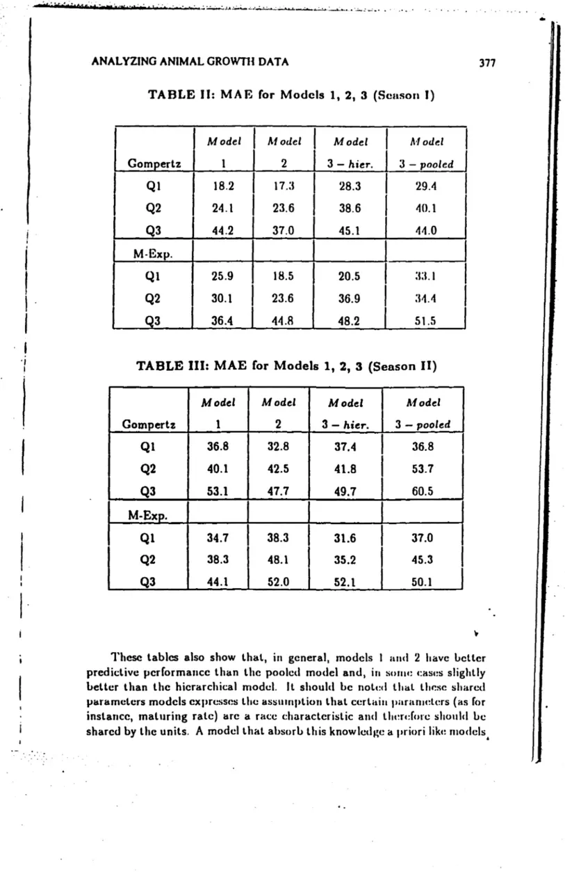
Frnrn 'li,ble ri ,uHI 111, ｬＧｦｬｉｮｾＬｬｉｬｉｬｉｬｩｬｬＬｾ＠ 1.0 t.WO ｃｬｩｦｲｦｾｲｬＧｬｉｴ＠ "itth ｓＧｾｬＱＡ［ｏｉｬｓＬ＠

il is ､ｦｾ｡ｲ＠ thaL the hierardlinll IIlmld ltas a Iwtll!r Iwrf"rrrlHlIl'(' tltan t.l1I! poolf!C1 model almost incfepf!fU"!nl.ly nf Ulf' fllrll'liollal fonn eonsidl!I'f'(1, wlr:ll RIlRR(!!llR lhe I1sefulncss of tlw ｰｔｃｬｰｦＩｳＬｾ､＠ hif!rard.kaJ rrwthndnlol'S. /t shollld

IIc ＱｬＰｬＨｾ｣ｉ＠ lhat this model ｬＩｦｾｲｬｬｬｩｴｳ＠ lo sllUllltari7.l! tlw inforrnalion I'olllairll'd in thl' flaln in " Illliqllc p'rnwl h 1'111'\"', '1111 ｫｦｾｾＢｩｬｬＬｾ＠ lll!' "npa\'ility "f ｴｗｬｫｩｬｬＬｾ＠

iufl!l'f'nf'I':i nf f!IU:h indivicllll\l ｳｬﾷｬｭｲ｡ｬＮＡｾｬｹＮ＠

"

•

.,

I

I·

ANALYZING ANIMAL GROWTH DATA 377

TABLE 11:

MA

E

ror Modcls

1,

2, 3 (Senson J)

Model Model Model Model

Gom ertz 1 2 3 - hier. 3 - pooled

Ql 18.2 17.:1 28.3 29.4

Q2 24.1 23.6 38.6 40.1

Q3 44.2 37.0 45.1 4-1.0

M·Exp.

J

I

Ql 25.9 18.5

I

20.5

I

a:1.

1

I

Q2 30.1

I

23.6 36.9

I

:HA

I

Q3 36.4 44.8 48.2 51.5

TABLE 111: MAE for Models 1, 2, 3 (Senson 11)

Mode' Mode' Model Model

Gompertz 1 2 3 - hier. 3 - pooled

Ql 36.8 32.8 37.4

I

36.8

Q2 40.1 42.5 41.8

I

53.7

Q3 53.1 47.7 49.7 60.5

M-Exp.

Ql 34.7

I

38.3

I

31.6

I

37.0

Q2 38.3 48.1 35.2 45.3

J

Q3 44.1 52.0 52.1 50.1

Thesc tablcs also show thal, in general, modcls 1 aluI 2 have Leller

predictivc performance lhan lhe poolcd model and, in SUIIII! c:asc:s slighlly

Lellcr lhan lhe hicrarchical mode!. Il should Le nolc:d lhal lhf!sC shared paramclcrs modcls expresses lhe assllrnplion lhal ccrlaill paralllders (as for

inslancc, rnaluring rale) are a race charactcrislic and ｴｬｬｬｾｲ､ＨＩｲ｣＠ shollld Le

sharcd by lhe unils.

A

modclthal absorL lhis knowletlge a I'riori likc: moclels,

•

378

•

1

0,8

0,1 0,4

• • • , ' « h ' • . •

...

ｾｾＺＺＺＺＺＭ

...

,

..

..

_{, ,}

.

_.

_.

, _,

,

, , _,

_,.

, _,

.

.

,

,

, _{, ,} ,

, ,

.

_,

"

.

..

_{. .}

"

...

'0 _O,.

.. ... .

BARBOSA ANO MIGON

ｏＬＲｾＭＭｾＭＭｾＭＭｾＭＭｾＭＭＭＴＭＭｾｾＭＭｾＭＭｾＭＭｾＭＭｾ＠

1 2 S 4 5 6 7 e t ｾ＠

_'li

••••• MlnimumIMulmum - Hlerarchlcal - Pooled

"G.1-Poeterlor ... .., tor th. Thlrd Par ... ter

(S .. eon I'

1 and 2, makes a beller use of ･ｘｉＩＨｾｲｩｬｬｬ｣ｮｬ｡ｬ＠ inforlllalion and lhcrcforc, il is

nol surprising lheir superior prediclive pcrformanr.r..

It should be stressed lhe fael lhal lhe hierarehieal model (V2

t

O) and

lhe shared parameler models in fael are useful lo approach eomplementary queslions. The shared paramelcr models are more effeelive for predielion

and lhe hierarchical model is more adequale lo summarize lhe informalion

relaled lo a11 individuais (of a eerlain race).

In order lo exemplify lhe aggregalion dilcrnma it i5 ｰｲｾ｣ｮｬｲＮｯ＠ in figure

I. lhe graphic of lhe poslerior mean of lhe ti' I'ararncler evalualed from

lhe univariale models and from lhe hir.rarchkal ano poobl lIIocld!l. Thr.

dollerllines represcnl lhe minimum Il.nd maxirnuUl ｯｨＡＡｲＮｲｖｴｾ､＠ valucs from lhe

univariale analysis for lhe 10 unil5 con!!idcred in lhe sca!!OIl 1. Thc olhers

represenl lhe poslerior mcan evolulion, ｲｾｰ｣ｲＮｴｩｶ､ｹＮ＠ for lhe h ir.rarchkal

model (fullline) and lhe poolcd modcl (hroken line). Il i!! dr.ar, a!l expccled, lhat lhe eslimates from lhe mullivarialc modc\s are more slable and slIloolh lhan lhe ones oblained from lhe univariale moclel!!.

5. FINAL REMAIlKS

Jl is worth lo slress ti,,: nmill ｦｩｬｬ､ｩｬｬｾｳ＠ ilIHI (·(lnclIlSiolls ｗＨｾ＠ f"alJ r.d flom

this application and lo slate souu: rdevnnl poillls for ｲｵｲｬｬｬｬｾｲ＠ illv(!sligalion .

.

.

,

ANAL YZING ANIMAL GROWTIf DATA 379 One of lhe main aspecls of lhe dass of proposcd ",odcls considerc,l in lhis paper is il grcat flexiIJilily. Firsl, lhis dass of rnoelels has a varidy of

par-ticular and uscful modcls

｣ｭ｢Ｈｾ､､ＨＡｴｬ＠

in il, dcfincd by difTcrcnl fllnclional

forms and difTerenl cxchangcahilily asslllllpliollS. A Iso, for a choscn func-lional form and a givcn himarchical slruclurc, lhe timc varying paramelers can accommodale difTerenl quanlilalive aspccts of lhe growth processo An-other imporlanl aspcd is lhe facl lhal lhe paramelers have a biological inlerpretalion.

As

expected ali models pcrform bellcr lhan lhe pooled model for dala

sets corrcsponding to caeh birlh season. For our objcclivcs, wc c:an say

lhat hicrardaical ",CHlcls aud sharc:,1 paramder JIIotlcls are in ｾｏｬｬｬｴＺ＠ sensc,

complcmenlary, sincc lhe lwo versions of modcl 3 are approprialc for dala descriplion and comparison (betwccn scasons), and mo deis 1 and 2 are more adequale for prediction.

One of lhe poinls for furlher work is lhe inclusion of an extra levei of hierarchy in lhe modcllo conlemplalc lhe efTects of differenl birlh seasons.

Wc ahould nolc lhat UU! proJloscd modds, condilionally on lhe valuc

of lhe

ｾ＠

parameter wOllld bc linear and conseqllcntly an allernalive form

of analysis could make use of the Gauss-lIcrmilc numerical inlcgration over

ＨｾＬ＠

V2). lIowever, lhis approach wOllld be morc sClIsible only for models

wherc V2 has few non-zero c1cmcnls. A ltt:rnativcly, lhe cslirnalion of V2

could be carried oul lhrollgh Markov chain Monle Carlo lc:chnology, in lhe dynamic conlexl as considered here.

BIBLIOGRAPIIY

Barbosa, E. P. '" lIarrison, P . .1. (1992) - Variance Eslimalion for

Mulli-variale Dynamic Linear Modc1s. .Jourllal of Forecasling, vol lI, 7, 621-628.

Blallberg, R.C

&

George, E.1 (1991), Shrinkage Eslimalion of Price and

Promotion Elaslicilies: sccrningly unrclalc,l equalions. Journal of the Arnerlcan Statistical Association, 86, "'1"', :10"'-315.

Fitzhugh, H.A (1976) - A nalysis of growl h curvcs ands slralegics for allering lhcir shapcs. Jonrnal of Animal Sciellce, 42, ....

Gamerman, D &t. Migon, II.S (1993), Dynamic Ilierarchical Models .•

lour-nal of the Royal Statistical Society, U, 55, 3, 629-642. •

Langc, N., Carlin, B.P &. (;c1fan<l, A.E (1!)!)2), llierachicallJaycs Modcl for

lhe Progrcssioll of HIV l .. feclion llsing Longiludinal CD4 T-Ccll

Num-bers. Journal of the Alllcricall Statistical Associatioll, 87, 419.

Lindley, O.V &to Smilh, A.M.F (I!J71). Bayes Eslimatcs for lhc Lincar Mo,ld

(wilh discussioll) . .1ournal of the Iloyal Statistical Socicty, 11,34, 1-41.

ｾＮ＠

380 BARBOSA ANO MIGON

Migon,

n.s

1.1. Uarbo!la,

RI'.

(1994), Non-linear Dynamic Modcl!; with

Ap-vlication to Growlh Curves. Itcl.Tec., LES, UFRJ.

Migon,

n.s

&. Gamerman, f) (1991), Generalizcd Exponcntial Crowth

Mod-eIs - a Bayesian approach. Journal of Forccal'iting, 12, 573-5R4 .

Racine-Poon, A (19R5), A Uaycsian Approach lo Non-Lincar Itanclom Errccl

ｾ＠ Modcl!l, BiolllctricR, 41, 1015-1023.

ｗｾｬＬ＠ M 1.1. lIarrison, P . .J. (1989), Daycsian Forccasting and Dynarnic Models, Springcr- Verlag.

r

I

I ｾ＠

h

_\,

.

.1

Uma Aplicação de lvIétodos de Monte-Carlo em Modelos de

Volatilidade

Hedibert Freitas Lopes (IM-UFRJ) Hélio S. Migon (IMjCOPPE-UFRJ)

Abstract

Os modelos para séries temporais heterocedásticas têm sido explorados exaus-tivamente na última década. Engle (1982) e Bollerslev (1986) observaram que as . mudanças na volatilidade de várias séries tendiam a ser serialmente correlacionadas e propuseram, respectivamente, os modelos ARCH (Autoregressive Conditional Het-eroscedasticity) e GARCH (Generalized ARCH).

O mais popular desses modelos é o GARCH(l,l), onde a série de interesse bt} é um processo ruído branco gaussiano com variância unitária, {td, multiplicado por um fator de escala {(J t}, isto é,

IIt

Ｈｊｾ＠

(Jt€t, t = 1,···, T, tt"" N ID(O, 1)

ＭｹＫｑｉｉｾＭｬＫｻＳＨｊｾＭｬＧ＠ -y>0, Q+{3<l.

(1)

(2)

Este modelo pode ser estendido adicionando-se mais defasagens de Yt e Ｈｊｾ＠ na e«uação (2), embora seja pouco comum nas aplicações. Quando (3 =

°

temos um ARCH(I).

Os principais fatores que podem explicar o crescente interesse nesta área são:l

1. O reconhecimento de que muitos modelos teóricos em finanças e8tão relacionados a volatilidade; por exemplo, os retornos de investimentos em ações e as taxas de câmbio exibem, em geral, mudanças na volatilidade ao longo do tempo.

2. A modelagem da volatilidade é um excelente campo para o desenvolvimento c aplicação de novas técnicas estatisticas para modelos não-lineares e não-gaussia-nos2•

Geweke (1989) e Müller & Pole (1994) estudam os modelos GARCH sobre o en-foque bayesiano; Geweke utiliza técnicas de integração Monte Carlo com Importance

Sampling, enquanto Müller & Pole utilizam Métodos Monte Carlo via Cadeias de

Markov.

Uma alternativa aos modelos ARCH é permitir que a} dependa de algum compo-nente não-observável ou variável latente modelando seu logaritmo (isto é, ht

=

ｬｯｧＨｔｾＩＬ＠

através de um processo estocástico linear. Modelos de8se tipo são comumente chama-dos de Modelo! de Volatilidade E!toclÚtica (SV). Esses modelos são uma versão, em tempo-discreto dos modelos que governam a maior parte da teoria moderna de finanças (Taylor (1993)).

1 Existem centenas de artigos publicados sobre o temlL

2Carlin, Polson &: Stofrer (1992) ､ｦｧ･ｮｹｴＩｬｾｲ｡ｭ＠ métodos de estimação de modelos dinâmicos nâo-lineares e nâo-normais 1m&Ildo Gi""! Sampling.

1

81BUOTECA MARIO

HENRIDUE SIMONSEI

Uma versão simples de modelos de volatiJidade estocástica foi proposta por Taylor

(1986):

YI

ht

exp{ht!2}EI' t= 1,···,T, Et "-'NID(O,l)

'"Yo

+

'"Ylht-I

+

IIt, 111 '" (O, ｵｾＩ＠

(3) (4)

Uma interprt'tação da variávt'llatent.e ht f. rf'presentar a variação irrf'gular e aleatória de novas observações, o que é muito difícil de se modelar diretamente em mercados financeiros 3.

O modelo SV pode ser re-escrito como

ht

+

log{En

'"Yo

+

'"Ylhl - I

+

111

o qual pode ser pt'nsado como um modelo dt' espaços de estado.

(5) (6)

A facilidade de avaliar a função de verossimilhança e sua adaptação para muitas séries temporais econômicas tomou os modelos ARCH muito populares. Por outro lado, a dificil avaliação da função de verossimilhança dos modelos de volatiJidade estocástica dificultaram sua aplicação empírica".

Recentes esforços têm sido feitos para reverter esse quadro, uma vez que, como já foi dito, os modelos SV têm boas propriedades, pelos menos quando se trata da sua adaptação a situações econômicas empíricas. Jarquier, Polson & Rossi (1994) abordam o problema sobre o enfoque de Modt'los Hieráquicos Bayesiano, isto é: p(1I1

I

hr}, p(h,

I

w) e p(w). O exemplo apresentado em (3) e (4) corresponde a

(Yt

lu;)

(ht

I

w)

(w)

NIO,

u:1

ｎｬｐｴｬｏＢｾＱ＠

p(w)

onde: ｵｾ＠

=

exp(ht), I-'t

=

'"Yo

+

'"Ylht -I e "-'

=

bOI

'"YI, UII).

(7)

(8)

(9)

Este trabalho tem como primeiro objetivo fazer uma comparação das representa-ções mais simples vistas acima, onde a estimação é feita através de dois procedimentos de integração: (i) Amostrador de Gibbs e (ii) ｓ｡ｭｰｬｩｮｧＭｒ･ｾ｡ｭｰｬｩｮｧｱｵ･＠ gera amostras

de b, a, tJ) ou bo, '"YI, 0"11) da priori, amostras estas que são reponderadas pela função

de verossimilhança e tranformadas em amostras da posteriori, onde toda análise é então concluída. Essa última técnica (chamada de Sampling-Importance Resampling (SIR), quando ligada a uma Importance Function), tem um grande apelo pedagógico e sugere uma estratégia de cálculo fácil de implementar (Smith & Gelfand (1992). Fazemos esses exercícios com uma série simulada com uma estrutura na volatilidade e com algumas séries da economia brasileira.

30 interesse em modelar volatilidade já vem de longa data, com o trabalho de Clark (1973) que propõe um modelo de misturas para a di.'1tribuiçiio das mudanças nos preços de ações.

4Kim & Shepard (1994) e Shepard (1995) fazem extellSAS revisões dos principaL'! conceitos, técrúC88 de estimação e -previaio e desafioe que estão por traz doe modelos ARCH e dos modelos SV.

•

UMA A.PLICAÇÃO DE MÉTODOS DE MONTE CARLO EM

,

MODELOS DE VOLATILIDADE ESTOCASTICA

Helio

S. Migon

e

Hedibert

F. Lopes

Universidade Federal do Rio de Janeiro - IM

&

COPPE .

e-ma.il: migon at pep.ufrj.br

CONTEÚDO

Introdução

1. Modelos ARCH e de Volatilidade Estocástica:

exemplos e propriedades básicas

2.

Uma

Classe Geral de Modelos de Volatilidade Estocástica

3. I .. ferência em Modelos de Volatilidade Estocástica

4. Exemplos:

Usando dados artificiais

Usando dado real:

taxa de juros

5.

Extensões e Conclusões

4-•

..

I

,.

I

TRODUÇAO

Motivação

• Teoria moderna de finanças propõe modelos de decisão relacionados

com a volatilidade.

• Modelos de volatilidade são excelentes exemplos de modelos

nã.o-li--

.

nea.Jes e nao-norm8.1s.

• Em modelos dinâmicos é comum modelar-se a variância observacional.

Objetivos

• Investigar uma ampla classe de modelos de volatilidade estocástica

-uni e multivariado..

• Propor métodos de estimação Bayesiana e comparar resultados.

• Discutir tópicos de seleção de modelos via fator de Bayes e medidas de

não linearidade.

• Avaliar influência usando medidade de Kullback-Leibner

1.

ｬ｜ＴｧｰｾｾＮｏｳＮ＠

ａｾｊｪ＠

ｾ＠

PE

VOLATILIDADE ESTOCÁSTICA

MODELO ARCH(l)

1/2

Yt

_.

=

I1:t ft,

_. ft ""

n[O,

11

.

Alternativamente

2 c 2

Yt

=

a

+

u

Yt-1

+

Vt,

Propriedades

,]( _

E[y11

_

3(1 - 6)

se 36

2

<

1

- E2 [Y;

1 -

1 - 36

2 '

• 11;

é covariância-estacionário com função de autocorrelação:

• Yt

é ruído branco se:

Ó

<

1

...

ｾＮ＠

__ .. __ ...

｟ＭＭＭＭＭＭＭ］］］］］］］］ＮＮＬ［ＬＭ］Ｍ］］Ｎ］Ｍ］Ｎ｟Ｎｾ｟＠

.... _ ... _--_ ..

ｾＢＢＬ＠

.

,

Co

h

1/ 2

Yt

=

t ft, ft '"

n[O,

1

J

I1t

=

O'

+

6

Y;-1

+

cP

ht-l'

O'

>

O

Alternativamente

Propriedades

K

-

E[ytJ

_

3 3

var[E[y;

IYt-dJ

- EJ2

[y;]

-

+

E[y;)2

,

• y;

é

covariância-estacionário com função de auto correlação:

1 -

6(6

+

cP)

py:(l)

=

1

+

6

2 -

26(0'

+

cP)

•

Ｑｗｒｩｪｊｙｾｏ＠

DE VOLATILIDADE ESTO,CÁSTJCA LQG-AR{l)

VE8T - LOG-AR(

1)

'l't

=

log(ht)

Alternativamente

MODELO DINÂMICO NÃO NORMAL E NÃO LINEAR

com hiperparâmetros

w

=

(a, ó,

ｵｾＩ＠

Propriedades

E[ytl

2 a 2

ｵｾ＠

K

=

.E2

[y;l

=

3 exp(

U \li ,

ｊＱＮｾ＠

=

1 _

Ó

e

U

ｾ＠

=

1 _ 6

₂

• y;

é

sinlllar a

ARMA(l,l)

com função de auto correlação:

VEST é similar ao GARCH(l,l)

• Yt

é ruído branco se:

Ó

+

4>

<

1

-,

---onde:

2. UMA CLASSE GERAL DE MODELOS

DE VOLATILIDADE ESTOCÁSTICA

(Yt

Ih..t)

rv

EF[O, ht]

(h

t

10,0-;,

Dt-d

rv

[JL(O,

Dt-d,

ｏＢｾ｝＠

ｰＨｏｉｏＢｾＩ＠

ｰＨｏＢｾＩ＠

7

• ( J -

é

qualquer distribuição sobre

R+,

especificada pela média e

vuiância, EF - familia exponencial e

• D"_l

=

(Yl,' . "

Yt-lt

h

1 ," "

ht-d

Se desejável

O

pode variar no tempo

,

MODELO HIERARQUICO

•

•

I ,

.

f

• ARCH(l)

• VEST-AR(l)

EXEMPLOS

J.L(8,Dt-d

=

0'+6

Y;-l

(J2 _v ===?

O

J.L(8, Dt-d

=

O'

+

6

log(ht-d,

ｖＨｊｾ＠

(h

t

10,

ht-d

'"V

LN[J.L,

ＨＷｾ｝＠

• VEST-NORMALjGAMA AR(l)

(Yt Iht)

'"V

N[O, ht]

(ht Iht-d

'"V

Ga[J.L(O, Dt-d,

ＨＷｾ｝＠

J.L(8, Dt-d

=

O'

+

6

log(ht-d,

'V

ＨＷｾ＠

• (O'

+

6

ht_l)2

at

=

2

(7v

•

, !,

I I

o

T-a

o

ｾ＠

q

;'D

: ｾ＠

ｬｾ＠

o

o

C

O

--- -

ＭｾＭＭＭＭＭＭＭＭＭＭＭＭ｟ｺ＠

_{Figura 1:}

___ _

(a) Série Original (T=250) e Função de

auto correlação

(FAC)

(b) Série Transformada (quadrado)

e

Função de

auto correlação

(FAC)

ｾｾ＠

---50

100

200

co

u. '

U o

<:

J

1

·i·· .i.

N_·:!_..I_ .. L_ .. __ .. ___ . __ . _____ .. __ .. __ .. _ ._ ...

o

I

co

u.' U O

<:

o

o

o

,5

_10.

₁₅

₂₀

Lag

Series : yarc952

-1 i··· ---··-·-:lii ...--_. __ ... ..Li

.. .... .. .- . . ... __ . ....

-

. ... . Ｍｾ＠ . __ ... _ .. _ .. -.

o.

50 100

₂₀₀

o.

₅

_10.

₁₅

₂₀

Lag

-,

1

•

l

1

I .

I

r

o

('t)

I

. ｾＮＮＮＭＭＭＮＮＭ

- - -

_

....

__

.- ...

ｾ＠ .

,

1titií

igura 2:

(8.)

Série Original

(T-250)

e Função de auto correlação (FAC)

(b) Série Ttansformada (log-quadrado) e FUnção de auto correlação (FAC)

o

50

100

200

o

50

100

200

T .-

52

II

I

.-t

<D

u.

0

(J0

c:(

o ..- .. --- .. -. ... I .. t

o ...

J ._ J .... __ I ..... _ ... _ ... __ .. ｾｬ＠ __ . __ L.

<D

u.

0

(.)0

c:(

o

o

o

o

5

10

15

20

Lag

Series : ysv9821

5

10

15

20

Lag

'aO' ... .

,

.

r

"1.

..

Ê

3. INFERENCIA EM MODELO DE VOLATILIDADE

ABORDAGEM BAYESIANA

SAMPLING IMPORTANCE RESAMPLING

Unl algOrítÍlllO aplicável tanto elll nlOdelos ARCH como VEST é

de-scrito por

i) Gerar

N

pontos da distribuição a priori

O,

rv

p(O)

i =

1 ...

N

1 , "

ii) Gerar, no caso VEST, N pontos da distribuição de evolução das

volati-lidade

lI'rvN[O

1 "

1] i - I .. ·

- , ,

N

iii) Calcular as realizações da volatilidade

iv) Obter os pesos gerados pela verossimilhança

exp(

wi)

Wi

=

,

onde

ｾ･ｸｰＨｷｮ＠

2

wi

=

Ｍ｛ｾ＠

log(O';,d

+

ｾ＠ ｹｾ＠

]

O't '

,1

v) Gerar M pontos a partir da distribuição discreta

{Oi,wd

ＨＩｾ＠ rv

P(()l

...

()N)

i = 1 ...

N

e

J'

= 1 ... M

..

AMOSTRADOR DE GIBBS

Modelo de Volatilidade Estocástica

Posteriori Conjunta

p(h,wly)

ex

p(ylh)p(hlw)p(w)

Condicionais Completas

p(

w

Ih, y)

==>

Modelo Linear Bayesinao

p(hlw, y)

==>

Fazer

Passo

a

Passo

p(ht Iht-1' ht+1' w, yt)

=

p(ytlht)p(ht Iht-dp(ht+1Iht)

=

h;1/2 exp[-y; /2ht]1/ht exp[-(Iog(ht)

-

I1t)2/(210g(0-2)]

onde:

I-l

=

[a(l -

6)

+

6(log(h

t

+

1

+

log(ht-dl/(l

+

6

2 )

0-

2

=

_{ＰＭｾＯＨＱ＠}

-

6

2₎

7

-._---4.1. DADOS ARTIFICIAIS

Modelo

ARCH(l)

• Série gerada COIn parâmetros

Q'

=

0.00015,

Ó

=

0.95 e

T

=

250.

• SIR,

conl priori não infonnativa (bem escolhida!), fornece

resul-tados lllaiS razoáveis que o lllétodo de lnáxinm verossimilhança,

COlll inicialização (0.00015,0.95) extremaxnente precisa.

RESULTADOS OBTIDOS

Ｎｉｾ＠

__

ｾ＠

______

S_I_R ______

ｾ＠

______

M_L_E ____

ｾ＠

I

Q'

0.000173 (0.000025)

0.00016 (0.0000089)

I

Ó

0.902386 (0.062271)

1.0316 (0.16250)

• Observe que

Ó M LE

>

1, inlplicando enl processo não estacionário,

além da convergência ser fraca.

• Gibbs Salllple: o prograllla utilizado, BUGS, não consegue

veri-ficar a log-concavidade, elnbora esta seja garantida.

---_._--_.-_._---

kernel density for alfa

(5000

values)

kernel density

fOi"

gama (5000 values

•

o

o

o

lO

T""

o

o

o

o

T""

o

-o

..

•

o

lO

o

0.00005

0.00020

alfa

mean

=

O. 0017: s.d

=

0.000 2476 5%

=

0.00 139 95%

=

0.0 0221

•

N

o

mean

=

0.9024 s.d

=

0.06228 5%

=

0.7909 95%

=

0.997

0.7

0.9

gama

odeio VEST-LOG-AR(l)

• Série gerada com parâmetros

Q'

=

-0.245,

Ó

=

0.98

p ｏＢｾｵ＠

=

0.5, com

ho

=

1.0 e

T

=

250.

RESULTADOS OBTIDOS

• SIR,

com priori não infonnativa (bem escolhida!) e supondo

ｏＢｾ＠

conhecido

• MCMC via Bugs, com 3000 iterações.

SIR

MCNIC

Q'

-0.4723 (0.3381)

-0.4155 (0.1548)

Ó

0.8851 (0.0565)

0.9042 (O.O:3G4)

A -2

0"1/

2.00

fixo

3.19 (1.1030)

• Esses resultados, embora preliminares são anilll<lclores.

• Os rnétodos tem COlnportarllento sinular.

• Os intervalos de probabilidade de 95% pratiCéll1H'llt,C' contém ()

•

M ti ("'11 ti o ti o N o ti

ＭＭＭＭＭＭＭＭＭＭＭＭＭＭＭＭＭＭＭＭＭＭＭＭＭＭＭＭＭｾ＠

Volatilidade Estocastica

kemel density for alfa (3000 values)

-8

man - -4.167

s.d-0.9847

5% = -6.041

95% = -2.755

alfa

-4 -2

kemel density for tau2 (3000 values)

0.0 0.4 0.8

tau2

mun - 0.5123 s.d-O.l359 5"- 0.3321

95"-

0.7Sn

1.2

kemel density for gama (3000 values)

o

me.n- 0.729 s.d -0.06381

5%- 0.6058

95%- 0.8206

0.5 0.6 0.7 0.8 0.9

gama

kemel density for h[227] (3000 values)

o o o

11)

o _o

o M o o o

....

o 0.0

rnun - 0.00001 s.d - 0.00003434

5% - 3.828e-006

95"- O .. ｏｏｏｏｾ＠

0.0005 0.0010 0.0015

h[227]

ｾ＠

__ ﾷＳＮｾ＠

ｾ＠

__ • 0.0000146

ｾ＠

Ｎ､ﾷＷＮｾ＠ I.d· 0.00001&17

5'11 - 1.766e-«J7 N _5'11=

3.6828-006

95'11-ＰＮＰＰＰＰＱｾＲ＠ 95""-O()()()()4()23

ｾ＠

ｾ＠

ｾ＠

ｾ＠

_ｾ＠

•

O O

• _{0.0 0.00005 0.00010}

000015 0.00020 0.0 0.0001 0.0002 0.0003

h{(23) h(224)

kemel density for h[225] (3000 values) kemel density for h[226] (3000 values)

ｾ＠

__ - 0.00001152

ｾ＠

_{'""" - o.oooolm}

• d' O.oooolgca I.d • O.ClOO1:lZ&4

ＵＧＱＱﾷｧＮｾＷ＠

ｾ＠

ｾＧｉｉﾷＲＮｉｾ＠

_ - 0.000041 _ - o 0000!5405

ｾ＠

ｾ＠

S

ｾ＠

ｾ＠

O O

ｾＮＰＰＰＱ＠ 0.0 0.0001 0.0002 0.0003 0.0004 00005 00 0.0002 00004 00006

1\(225) h(226)

kemel density for h[227] (3000 values) kemel density for h[228] (3000 values)

ｾ＠

f\

'""". OoooolM4

ｾ＠

_ - 6.151e-406

I.d - 0.00003434 I.d· 0.00001_

S

ｾＧｉｉＭＳｾ＠ ＵＧｉｉﾷＳＮｉｾＷ＠

_ - O.CIOOO6389 15'11- 0.00002081

ｾ＠

_ｾ＠

ｾ＠

ｾ＠

\

•

O o

.

00 0.0005 0.0010 0.0015 00 0.0001 00002 0.0003 0.0004

h(227) h(228)

c'I

a

t == •••

".':22·! ..

r!B! ! ! ! -

-

e

..

-•

•

•

..

_.

UI

rraws

!!!Z!z=:::=tt . r . , _ _ ＧＭＭ｟ｾ＠ • • _ _ _ _ _ _ _ _

4.2. DADO REAL - TAXA DE JUROS

Esse conjunto de dados refere-se a taxa de juros de CDB pré-fixado (tres

dias úteis), isto é

10g

(

1

+

it!

100). A presentaulOs abaixo

UIlIa

análise usando

SIR e m modelos ARCH

COlll

U1ua estrutura AR( 1) para cuidar da não

estacionariedade da série original. Alguluas comparações são apresentadas .

• MODELO UTILIZADO

Yt

=

PYt-l

+

ｨｾＯＲｅｴＬ＠

Et '"

N[O, 1]

ht

=

a

+

6Y;_1'

Yo

=

O

• SIR,

COlll

priori não informativa ( bem escolhida!), fornece

resul-tados luais razoáveis que o lnétodo de máxinla verossimilhança,

COln

inicialização obtida de uma rodada de SIR que degenera,

(p,

Q,

6)

=

(0.736,0.00156,0.3473)

ｾ＠ ｲＭＭＭＭＭＭＭＭＭＭＭＭＭＭＭＭＭＭＭＭＭＭＭＭＭＭＭｾ＠

o

...

o

...

c:i

o o ｾＭＭＭＭＭＭ ________________ ＭＭＭＭｾ＠

o 50 100 150

..

_o N

.,;

.,;

o

o

o 50 100 150

- I

tE)

o

lO.

U ...

.. o

lO. U c o o ., o

...

o o o o O

_ 1

I

I

5 lO 15 20

Series : juros2

II

I

I

I I J I I I I I i _ｉｾｉ＠

5 lO 15 20

•

•

p

RESULTADOS OBTIDOS

SIR

0.9121 (0.042)

0.000325 (0.000092)

0.84499 (0.0184)

MLE

0.7636 (0.010)

0.000576 (0.000121)

1.40061 (0.2601)

• Observe que

6

M LE

>

1, iInplicando em processo não estacionário,

embora a convergência seja forte .

• Outras inicializações do luétodo de máxima verossimilhança não

converglralIl .

...

ｾ＠

..

ｾ＠

....

ＭＭＭＭＭＭＭＭＭＭＭＭＭＭｾ＠

•

• a

•

p

•

t

•

LO

ｾ＠

o

ｾ＠

o

•• ,( e • a .• · .. " .... ＭｾＧｾｾｾＢＢＧＭＢＧｾＭＧＧＧＡＧｐＧ＿ｐ］ｬｉＡＡＧｴＮ｟＠ ""'!"&-",. _ _ 0 _ ... _... ... ' .. 1 ...•• '''':ltJ!!as&J3d&2

• Resultados de VEST foraln obtidos no BUGS para um modelo sem

considerar a cOluponente de uiveI e, tanlbém, para mu modelo com

p

fixo. Esses resultados, elnbora razoáveis precisam ser melhor

analizados.

mean

=

0.9121 s.d

=

0.04217 5%

=

0.7973 95%

=

0.9846

0.80

0.90

alfa

•

1.00

o

o

o

c.o

o

o

o

N

o

mean

=

0.0003249 s.d

=

0.0000917 5%

=

0.000052 95%

=

0.000396

..

-0.0

0.0002

gama

- - - - -

---] ,I

•

•

•

-

-5. EXTENÇOES E CONCLUSOES

• Ivlétodos de Nlonte Carlo são dPt.ivos.

• Classe ampla de lllOdelos a iuv(·st.igar.

• Implenlentar técnicas de diagw')stico e seleção de 111O<1<'1os via Fator de

Leibner

• Representar lllOdelos ARCH em estrutura linear diu:ullica.

6. REFERÊNCIAS BÁSICAS

Jacquier, E, Polson,

N.G

&

Rossi, P.E

(1994) -

Bayesiull aI1êlIysis of

stochas-tic volatility lllOdels, JBES.

Nlills, T. C

(1993) -

The ecollOllletric lllodelling of fiallcial time series, CUP.

:tvluller, P

(1991) -

A clyllanlÍc vPd.Ol" ARCH lnodel for pxc-hange rate data,

ISDS Tec.Rep.

Tay lor, S

(1986)

Nlodellillg financiaI time series.

Shephard,

N

(1995) -

statistical aspects of ARCH and Stochastic Volatility, .

Disc.Paper

94.

.

.

@-!

Alln8i.&II I.Pi li' li' •• AA_a

N.Cham. P/EPGE SPE M636m

Autor: Migon, Helio S.,

Título: Modelos dinâmicos não lineares e aplicações de

088357

1111111111111111111111111111111111111111 51501

FGV - BMHS N° Pat. F3495!98

000088357

1111111111111111111111111111111111111

,

t

•

•

..

•