Abstract—Effects of a linear chirp and filter response on soliton propagation are considered in this paper based on the efficient method which is a combination of Fourier series analysis technique (FSAT) and Jacobi iterative method. In our simulations, some important effects such as fiber nonlinearity and dispersion are considered and results compared with a simple uniform fiber gratings.
Index Terms—Fiber Bragg grating, soliton, chirped structure, dispersion
I. INTRODUCTION
IBERBragg gratings (FBGs) are important elements in many optical applications when the spectrum compression, short pulse stretching, optical filtering and pulse spectrum shaping are needed [1]. These structures are used in optical fibers with numerous applications on dispersion management designation. By using FBGs with non-uniform grating period, or chirped gratings, it is possible to tune the fiber dispersion and its slope [2-6]. For the aid of dispersion compensation in bi-doped lasers, one can use FBG structure too [7]. An accurate spatial chirped structure can give ultra-short and nonlinear chirped micro-wave pulses [8, 9].
One of the important aspects of FBGs is the propagation of soliton pulses and effects of the fiber parameters, such as dispersion and nonlinearity, on them. These behaviors are described by a set of nonlinear coupled partial differential equations which are not integrable in general case. Many numerical methods are reported in the literature; for example the transfer matrix method (TMM) [10] and inverse scattering method (ISM) [11]. In the former method, FBG is divided by small parts so that any section can be defined by a simple
2
2
matrix. The matrix entries explain the interaction between the forward and backward pulses. Ultimately, the fiber action can be described by multiplication of all sectional matrixes. In this method, time dependent and nonlinearities are not considered. In ISMManuscript received Dec. 10, 2011. This work was supported in part by the optoelectronic research center, electronic department of Shiraz University of Technology, Shiraz, Iran.
F. Emami is with the optoelectronic center, electronic department of Shiraz University of Technology, Shiraz, Iran; (corresponding author, phone: 0098-711-7266-262; fax: 0098-711-7353-502; e-mail: [email protected]),
H. Bashiri is with the optoelectronic center, electronic department of Shiraz University of Technology, Shiraz, Iran; (e-mail: [email protected]),
Sh Kohan is with the optoelectronic center, electronic department of Shiraz University of Technology, Shiraz, Iran; (e-mail: [email protected]).
method, an analytical solution for the governing equations is proposed and based on some undefined solitary coefficients, the coupling equations are solved. Unfortunately, the mentioned methods are not general and for every input pulse with arbitrary shapes are not applicable. To overcome this problem, we proposed a numerical efficient method to simulate the pulse propagation in FBGs with any input pulses and in general conditions.
II. NONLINEAR CHIRPED FBG THEORY
Soliton propagation in FBGs is modeled by a set of coupled equations. A nonlinear index grating can be considered as:
) ( 2 2 ) ( ) ,
( z n n E ng z
n (1) Where
n
is the average linear refractive index,n
2 is nonlinear refractive index, E is electric fieldδ
n
g
z
is the refractive index variations of FBG along the propagation directionz. It can be defined for different gratings in various descriptions for example for a linear chirped FBG (LCFBG) it can be represented as:
20
2
cos
z
cz
z
n
n
z
n
g eff eff
(2)Where
n
eff is the background effective index,Λ
0is the grating period at the input end of the grating,δ
n
eff
z
is the index profile variations in the grating and
20
Λ
2
cz
π
Z
φ
is the grating linear chirp with thecoefficient of c. For a linear chirp FBG, the grating period can be assumed as:
z 0
12cz
(3)
Consequently, the Bragg wavelength is a function of the grating period along the propagation direction with the following definition:
z neff neff
z neff
z B 2 2 (4)
Generally, a grating can be modeled by the coupled mode theory. The forward and backward fields, Af and Ab, are found by the set of nonlinear coupled equations [12]:
Simulation of the Soliton Propagation in the
Linear Chirped Fiber Bragg Grating
F. Emami, Member, IAENG, H. Bashiri, and Sh. Kohan
F
) 5 (
)
(
2 2 23 3
6 3 2 2
2 2 1
f A b A A
t f A g
t f A g j
t f A g z
f A
f
g
j
b
A
j
f
A
j
) 6 (
)
(
2 2 23 3 6
3 2 2 2
2 1
b A b A A
t b A g
t b A g j t
b A g z
b A
f
g
j
f
A
j
b
A
j
g
1 is the effective first order dispersion factor,
g
2 is the effective second order dispersion factor (Group Velocity Dispersion or GVD),and 3g is the effective third order dispersion. They can be found from the following equations:
2 2 1 ) ( ) ( 1 1 ) ( z z v z g g
2 3 2 2 2 2 2 ] ) ( ) ( [ ) ( )) ( sgn( ) ( z z v z z z g g
2 5 2 2 3 2 3 ] ) ( ) ( [ ) ( ) ( 3 ) ( z z v z z z g g
(7)
In the above equations, δ is detuning factor that refers to deviation of Bragg wavelength from central wavelength, in the case of δ=0 FBG act as a filter with 100% reflectivity anddefined as:
)
)
(
1
1
(
2
)
(
z
eff
n
z
B
(8)Bis Bragg wavelength. g
is the nonlinear factor and increases for higher input pulse powers. Finally is the coupling coefficient and determines the amount of energy exchange between forward and backward fields:
z
n
π
z
)
2
eff(
)
(
(9) To solve these equations, we use the method named Fourier Series Analysis Technique (FSAT) .Assume a solution for Af and Ab in the form of: n n t jn e z fn a t z f
A ( , ) ( )
(10)t jn e n n z bn a t z b
A
( ) )
,
( (11) In the above equations each term of the field amplitudes decomposes into two parts; time and displacement. After substituting the selected solutions of (10) and (11) for the field amplitudes in (5) and (6) and choosing a truncated Fourier series (with N replaced by
, or equivalently 2N+1 term) we have:) 12 ( 1 2 1 ) ( ) ( ) ( ) 3 3 ( 6 3 ) ( ) 2 2 ( 2 2 ) ( ) ( 1 ) ( t jn e N n n t jn e N n N n n g j t jn e N n N n z a j t jn e z fn a j N n N n t jn e z fn a jn g N n N n t jn e z fn a n g j N n N n t jn e z fn a jn N n N n g t jn e z fn a z N n N n N n b n ) 13 ( 2 2 2 ) ( ) ( ) ( ) 3 3 ( 6 3 ) ( ) 2 2 ( 2 2 ) ( ) ( 1 ) (
t jn e N n N n n t jn e N n N n n g j t jn e N n N n N n N n z fn a j t jn e z bn a j N n N n t jn e z bn a jn g N n N n t jn e z bn a n g j N n N n t jn e z bn a jn N n N n g t jn e z bn a z Where t jn N N bn t jn N N bn N N t jn n N N t jn fn N N N N t jn fn t jn n e z a e z a e e z a e z a e
) ( . ) ( , ) ( . ) ( 2 2 2 1 t jn N N bn t jn N N fn N N t jn n N N t jn fn N N N N t jn bn t jn n e z a e z a e e z a e z a e
) ( . ) ( , ) ( . ) ( 2 2 2 1Multiply both sides of (12) and (13) by
e
jnωtand integrating on the interval
π
ω
t
π
ω
, we found two coupled equations fora
fnanda
bn as follow:
1 2 1
(14)) ( ) ( ) ( ) 3 3 ( 6 3 ) ( ) 2 2 ( 2 2 ) ( ) ( 1 ) ( n n g j z bn a j z fn a j z fn a jn g z fn a jn z fn a jn z fn a z
2 2 2
(15) ) ( ) ( ) ( ) 3 3 ( 6 3 ) ( ) 2 2 ( 2 2 ) ( ) ( 1 ) ( n n g j z fn a j z bn a j z bn a jn g z bn a jn g z bn a jn g z bn a z Our initial conditions for the above first order coupled equations for
a
fnanda
bn atz
0
are:
N n N n t ω jn bn b N n N n t ω jn bn b N n N n t ω jn fn fe
L
a
t
L
A
e
a
t
A
e
a
t
A
)
(
)
,
(
)
0
(
)
,
0
(
)
0
(
)
,
0
(
Essentially, the problem is the combination of initial and boundary value problem. Because of this difficulty, we guess the unknown coefficient such
a
bn
0
, and then we correct it by an iterative method. Multiply both sides of (16) bye
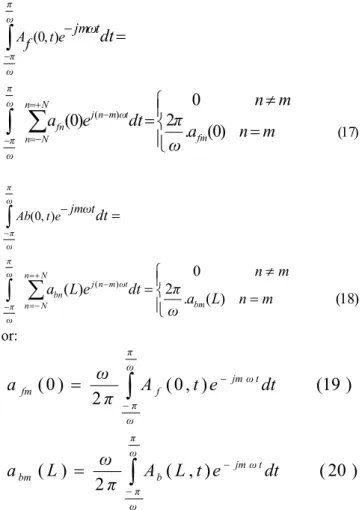
jnωtand integrate, we have:(16a)
(16b)
ω π
ω
π fm
N n
N n
t
ω
m n j fn
ω π
ω π
m
n
a
ω
π
n
m
dt
e
a
dt
tω
jm e t f A
) 17 ( )
, 0 (
)
0
(
.
2
0
)
0
(
( )
ω π
ω
π bm
N n
N n
t
ω
m n j bn
ω π
ω π
m n L a
ω
π n m
dt e
L a
dt
t
ω
jm e t Ab
) 18 ( )
( . 2
0 )
( ( )
) , 0 (
or:
)
20
(
)
,
(
2
)
(
)
19
(
)
,
0
(
2
)
0
(
ω π
ω π
t
ω
jm b
bm
ω π
ω π
t
ω
jm f
fm
dt
e
t
L
A
π
ω
L
a
dt
e
t
A
π
ω
a
To solve the (5) and (6), we should impose the boundary conditions on the structure. In fact, there are 4N +2 coupled equations (2N +1) for forward and 2N +1 for backward waves). Decomposing the real and imaginary parts of the elements, we have to solve 8N +4 coupled equations. We used the fourth-order Runge-Kutta method and Jacoubi iterative method, to solve the set of the coupled equations. At first, we guess a value for backward waves which inthis case (first step), they are determined. By using the mentioned method the Fourier coefficients of (16), are determined. Then with these new values of the variables the process is repeated. After a few times, the convergence is achieved and we can found the
A
f andA
b.III. SIMULATION RESULTS
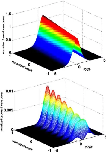
In this section we will apply the aforementioned method on an optical switch which uses a FBG. The input pulse was considered as sech (). We simulated two cases for pulse propagation in this structure . To test our method, at first we considered a uniform case without any chirp and nonlinearity in the structure which has reported results in the literature. The forward and backward wave amplitudes are plotted in Fig. 1. As seen, these pulses are propagated periodically and save their energies by interchanging powers between forward and backward waves.
Effect of chirp can be applied by defining ng
z as in (2)with different values of c. The results of our simulations in the case of small dispersions are shown in Fig. 2 and Fig. 3. It is found that there are narrower pulse width and lower peak for the structures with higher linear chirp.
Fig. 1 Soliton propagation in a uniform, linear non-chirped FBG
Fig. 3 Soliton propagation in a uniform, linear chirped FBG with the Chirp factor of 10x10-6cm-1
As shown, this technique can be used when compressed ultra short pulses are needed. With low dispersion values, the pulses are moved along z direction without any deviation along the time axis. Also a large amount of injected energy is exited from the end section of FBG and some energy is reflected.
The above results are repeated for higher amounts of dispersion. As expected, in the high dispersive media the propagated pulses deform during the propagation direction. It is shown in Fig. 4 and Fig. 5.
As seen, the peak power of propagated moving pulses shifts along the time axis. This is due to variations of group velocity. The shifting of the pulse power peak toward the right and left is for positive and negative1factor,
respectively. Also from Fig.4 and Fig.5 we found that increase dispersion, the propagated pulses along the fiber miss their oscillatory behavior and broadened. So, the pulses are widened and output peak power is lowered. Indeed, the pulse energy is constant in all cases and only power transmission is occurred between backward and forward oscillatory pulses; the wider pulse means lower peak power for pulse.
By comparing Fig.4 and Fig.5 with Fig.2 and Fig.3 we found that the quality of the compressed pulse should be better for smaller values of the fiber dispersion.
Fig. 4 Soliton propagation in a highly dispersive media-1
IV. CONCLUSION
In conclusion, we have proposed and simulated an effective method to study the pulse propagation in a LCFBG structure. Our method was based on combination of FSAT and Jacobi iterative method to solve the set of coupling equations. Results of our simulation confirm that there is a decrease in the pulse width and pulse power when linear chirp factor increases. In another case we used our method to simulate pulse propagation in LCFBG considering the dispersive effects. It is found that dispersion effects cause a shift of the propagated pulse along the time axis.
REFERENCES
[1] C. Wang, and J. Yao, “Fourier transform ultra-short optical pulse shaping using a single chirped fibre Bragg grating,” IEEE J. Photon., Tech., Lett., vol. 21, no. 19, Oct., 2009, pp. 1375-1377.
[2] S. Li, X. Zheng, H. Zhang, and B. Zhou, “Compensation of dispersion- induced power fading for highly linear radio-over-fiber link using carrier phase-shifted double sideband modulation,” Opt. Lett., vol. 36, pp. 546–548, 2011.
[3] R. Gumenyuk, C. Thür, S. Kivistö, and O. G. Okhotnikov, “Tapered fiber Bragg gratings for dispersion compensation in mode-locked Yb-doped fiber laser,” IEEE J. of Quantum Elect., vol. 46, no. 5, May 2010, pp. 769-773.
[4] Y. J. Lee, J. Bae, K. Lee, J. Jeong, and S. B. Lee, “Tunable dispersion and dispersion slope compensator using strain-chirped fiber Bragg grating, ” J. Photon., Tech., Lett., vol. 19, no. 10, May., 2007, pp. 762-764.
[5] M. Li, W. Liu, and J. P. Yao, “Continuously tunable chirped microwave pulse generation using an optically pumped linearly chirped fiber Bragg grating,” IEEE MTT-S Int., Microw., Symp., Dig., Baltimore, MD, Jun.2011, paper WEPL-1.
[6] W. Li and J. Yao, “An optically tunable optoelectronic oscillator,” J. Lightwave Technol., vol. 28, no. 18, Sep. 2010, pp. 2640–2645. [7] S. Kivistö, R. Gumenyuk, J. Puustinen, M. Guina, E. M. Dianov, and
O. G. Okhotnikov “Mode-locked bi-doped all-fiber laser with chirped fibre Bragg grating,” IEEE J. Photon., Tech., Lett., vol. 21, no. 9, May, 2009, pp. 599-601.
[8] C. Wang and J. Yao, “Nonlinearly chirped microwave pulse generation using a spatially discrete chirped fiber Bragg,” in the Int., Topical Meet., on Microwave Photonics, MWP' 09, pp. 1-4.
[9] M. Li, L. Shao, J. Albert, J. Yao, “Tilted fiber Bragg grating for chirped microwave waveform generation,’’ IEEE J. Photon., Tech., Lett., vol. 23, no. 5, March 2011, pp. 314-316.
[10] M. Yamada, K. Sakuda, “Analysis of almost periodic distributed feedback slab waveguides via a fundamental matrix approach,”Appl. Opt. vol. 26(16), 1987, pp. 3474–3478.
[11] A. B. Aceves, S. Wabnitz, “Self-induced transparency solitons in nonlinear refractive periodic,” Phys., Lett., A 141, 1989, pp. 37–42.