Towards The Development of an Index to Measure the
Performance of Multi-Productivity Areas
A.M. El-Kholy
Assistant Professor of Construction Project Management, Civil Eng. Dept., Faculty of Engineerig, Beni - Suef University, Beni - Suef, Egypt
ABSTRACT
This research aims to develop two models that predict the percentage loss or increase of productivity performance in construction firms. The first model based on regression analysis. Thirty-five factors that affected construction productivity gathered from literature and were found to be significant following a questionnaire survey. Twelve factors were the most significant factors that impact construction productivity (independent variables). An productivity performance index (PPI) was established (the dependent variable). The second model is a neural network model. Validation of the models revealed that out of 10 models tried by neural networks, the model with batch training, scaled conjugate gradient as an optimization algorithm and hyperbolic tangent and identity activation functions for input and output layers, outperforms the best model based on regression analysis. It gave Mean Average Percentage Error between the actual and predicted values of PPI by 12.5%, against 19.2% for the best model based on regression analysis.
Keywords:
Productivity Performance Index; Regression Analysis; Neural Network Model; Questionnaire Survey.I.
INTRODUCTION
One of the most important tasks confronting planners in the construction industry is the performance estimation of operations prior to commencement of construction. Productivity has been used as one criterion for explaining operational performance.
Productivity is defined by the business Roundtable (1982) as a ratio between output and input. A more general definition is offered by the ASCE committee on productivity, “delivery of a quality construction product that achieves total cost effectiveness through the optimise use of resources” (Kohn and Caplan, 1987). Productivity is an overall conception, which is difficult to express or to measure. It is sometimes expressed in terms of output from labour, or from services, or
from capital invested. Although they are
measurements of some or all of the inputs and outputs of the industry; but they failed to combine these measurements into any satisfactory measure of efficiency (Choy, 2009). Strandell (1982) defined productivity as “factor” or “total” productivity in which the former is the ratio of output to one type of input (labour, for example), and the latter is the ratio of output to all input factors (labour, capital, land and other investment). The definition of productivity as total productivity will be adopted in this research.
Strandell (1978) gave that construction professionals and owners agree that productivity in
construction industry is a problem that needs to be studied seriously because of its significance effect on the cost and duration of construction projects. Hope and Hope (1997) gave that productivity is the engine of economic both for a country and for an individual organization.
Researches on productivity could be categorized into two groups, the first group devoted to the factors influencing productivity. The second group deals with measuring and studying variability of construction labor productivity in
construction project and demonstrating the
conceptual benchmarking principles for
construction labor productivity. Examples for the first group are as follows. Olomolaiye et al. (1987) declared that the most significant factors in Nigeria are: lack of materials, rework, lack of equipment, supervision delays, absenteeism, and interference. Lim and Alum (1995) through a survey of contractors in Singapore found that the major problems with labour productivity are recruitment of supervisors, recruitment of workers, high rate of labour turnover, absenteeism at the work place, communication with foreign workers and inclement weather. Motawani et al. (1995) through a survey in USA found out that there are five major problems that affect productivity. These are: adverse site conditions, poor sequencing of works, drawing conflict/lack of information, searching for tools& materials, and poor weather. Zakeri et al. (1996) gave that lack of materials, weather and
physical site conditions, lack of proper tools and equipment, design, drawing and change orders, inspection delays, absenteeism, safety, improper plan of work, repeating work, changing crew size, and labour turnover are the most critical factors. Lema (1996) found that the major factors that influence productivity in Tanzania are leadership, level of skills, wages, level of mechanisation and monetary incentives. Kaming et al. (1998) found out that lack of materials, rework, worker interference, absenteeism, and lack of equipment were the most significant problems affecting workers in Indonesia.
However, Charamokos and Mc Kec (1981) reported that there are two main groups of areas, which have potential for productivity improvement, these are: head office and site. The factors related to head office are planning, procurement, scheduling, estimating, Specification. Site related areas include: labour relations, cost control, supervision, material delivery, material storage, material availability, labour training,
labour availability, recruitment, financial
motivation, equipment capacity, equipment
maintainability, equipment utilization, pre-cast
elements, pre-assemble modulars.
Makulsawatudom and Emsley (2002), reported that the most significant factors affecting construction productivity in Thailand are: lack of materials, incomplete drawings, incompetent supervisors, lack of tools and equipment, absenteeism, poor communication, instruction time, poor site layout, inspection delay, and rework.
Examples for the second group are as follows. Ibbs and Liu (2005) presented an improved “measured mile” approach which used to quantify losses in labor productivity. They analyzed the measured mile and the baseline method, and compared them to a new, proposed statistical clustering method. Abdel- Razek et al. (2007) improved construction labor productivity in Egypt by applying benchmarking and reducing variability in labor productivity. Several measures of benchmarks of construction labor productivity were demonstrated, calculated, and then used to evaluate the productivity of bricklayers and identify the best and worst performing projects. The benchmarks included disruption index (DI), performance ratio (PR), and project management index (PMI). The correlation between variability in labor productivity and project performance was also examined statistically. Lin and Huang (2010) introduced data envelopment analysis (DEA) as a new method for deriving baseline productivity (BP) and compares DEA with the other BP deriving methods. DEA was concluded as the best method in terms of objectivity, effectiveness, and
consistency to find BP that represents the best performance a contractor can possibly achieve. Liu et al. (2011) studied how work flow variation and labor productivity are related in construction practice. They found that productivity is not improved by completing as many tasks as possible regardless of the plan, nor from increasing workload, work output, or the number of work hours expended. In contrast, productivity does improve when work flow is made more predictable. Thomas and sudhakumar (2013) conducted a study on daily productivity of subcontract labor and directly employed labor for masonry works on a project. The results revealed that the subcontract labor achieved on an average 33% higher productivity than the directly employed labor. Idiake and Bustani (2014) examined the analysis of labor productivity data of block work activity from sixty one construction sites. The construction work composed of ongoing single story buildings in the study area Abuja metropolis. The variables :cumulative productivity, baseline productivity, coefficient of variation and project waste index were computed. The results showed that 44% variation in crew performance is accounted for by variability in labor productivity. Karmale and
Biswas (2015) studied the variability of
construction labor productivity in building
construction project and demonstrated the
conceptual benchmarking principles for
construction labor productivity. The study showed that the productivity rates of the construction workers vary from one project to another, taking into consideration the type of the activity to be carried out and the surrounding work environment. Recently, Hiyassat et al. (2016) described and analyzed the factors that affect construction labour productivity by conducting a questionnaire survey containing 27 questions (variables) on engineers and foremen who work for contractors. They statistically analyzed the returned responses by calculating the average, standard deviation of each variable. It was concluded that the top three ranked dimensions were „Productivity increases as experience increases‟, „Financial incentives increase productivity‟, and „Trust and communications between management and workers increase productivity‟.
Although a significant number of
researches have been conducted on both the factors that impact labor productivity and measuring &
studying variability of construction labor
productivity in construction project and
demonstrating the conceptual benchmarking
these areas in a construction firm. This reason stands behind the adoption of this study work.
In this paper, two models: regression based model and neural network based model for predicting productivity performance index for construction firms are developed. The independent variables are a number of qualitative variables that affect construction productivity gathered from literature. These variables are candidate according to their significance through a questionnaire survey. The next section presents the research scope and methodology adopted in this research.
II.
RESEARCH SCOPE AND
METHODOLOGY
In the current research two proposed predictive models are intended to be applicable for predicting productivity performance index for construction firms. These models are based on regression analysis and neural networks. A standard methodology will be adopted. As an initial step to meet the objectives, previous research papers that deal with factors influencing labor productivity, measuring and studying variability of construction labor productivity were reviewed in the previous section. The need for productivity performance index (PPI) which considers multi-productivity areas is explained in the next section. PPI is then developed. Artificial Neural Networks
are then described. Research methods in
construction are then discussed. A list of factors that affect construction productivity is prepared to collect data about significance of these factors through questionnaire survey. The next step is to analyze the survey results to obtain the most significant factors impact productivity to be incorporated into the predictive models. Building regression based model is then demonstrated and a numerical example is prepared to show how the model predicts PPI of a project. Neural network based model is then developed. The last step of this research is to validate the proposed models. Based on the validation results, the prediction accuracy of the two models is compared and conclusions are drawn.
III.
THE NEED FOR PRODUCTIVITY
PERFORMANCE INDEX
Productivity is commonly defined as a ratio of a volume measure of output to a volume measure of input use (Giovanni and Nezu, 2001). While there is no disagreement on this generalnotion, a look at the productivity literature and its various applications reveals very quickly that there is neither a unique purpose for, nor a single measure of, productivity (Giovanni and Nezu, 2001).
Productivity measurement is a prerequisite for improving productivity. Measures of Output could be in the form of goods produced or services rendered. Output may be expressed in: physical quantity or financial value. Physical quantity at the operational level, where products or services are homogeneous, output can be measured in physical units (e.g. number of customers served, number of books printed). Such measures reflect the physical effectiveness and efficiency of a process. Financial value at the organisation level, output is seldom uniform. It is usually measured in financial value, such as sales production value (i.e. sales minus change in inventory level) (Giovanni and Nezu, 2001).
Giovanni and Nezu, (2001) reported that productivity measures can be classified as single factor productivity measures (relating a measure of output to a single measure of input) or multifactor productivity measures (relating a measure of output to a bundle of inputs). Another distinction, of particular relevance at the industry or firm level is between productivity measures that relate some measure of gross output to one or several inputs and those which use a value-added concept to capture movements of output. Giovanni and Nezu (2001) reported measures of labour and capital productivity, and multifactor productivity measures (MFP), either in the form of capital-labour MFP, based on a value-added concept of output, or in the form of capital-labour-energy-materials MFP (KLEMS), based on a concept of gross output. The following paragraphs explain these measures.
Gross-output based labour productivity index given in Eq. (1) traces the labour requirements per unit of (physical) output. It reflects the change in the input coefficient of labour by industry and can help in the analysis of labour requirements by industry. One of it is advantages is the ease of measurement and readability. On the other hand, the drawbacks and limitations of labour productivity is that it is a partial productivity measure and reflects the joint influence of a host of factors. It is easily misinterpreted as technical change or as the productivity of the individuals in the labour force.
Q u a n tity in d e x o f g ro s s o u tp u t G ro s s o u tp u t b a s e d la b o u r p ro d u c tiv ity =
Labour productivity based on value added index given in Eq. (2) shows the time profile of how productively labour is used to generate value added. Labour productivity changes reflect the joint influence of changes in capital, as well as technical, organizational and efficiency change within and between firms, the influence of economies of scale, varying degrees of capacity utilization and measurement errors. Value – added based labour productivity measures tend to be less sensitive to processes of substitution between materials plus services and labour than gross-output based measures. This index forms a direct link to a
widely used measure of living standards, income per capita. One of it is advantages is the ease of measurement and readability. It is drawbacks and limitations are labour productivity is a partial productivity measure and reflects the joint influence of a host of factors. It is easily misinterpreted as technical change or as the productivity of the individuals in the labour force. Also, value-added measures based on a double-deflation procedure with fixed-weight laspeyres indices which suffer from several theoretical and practical drawbacks.
Q u a n tity in d e x o f v a lu e a d d e d L a b o u r p ro d u c tiv ity b a s e d o n v a lu e a d d e d =
Q u a n tity in d e x o f la b o u r in p u t
(2)
Capital-labour MFP based on value added index given in Eq. (3) shows the time profile of how productively combined labour and capital inputs are used to generate value added. Conceptually, capital-labour productivity is not, in general, an accurate measure of technical change. It is, however, an indicator of an industry‟s capacity to contribute to economy-wide growth of income per unit of primary input. In practice, the measure reflects the combined effects of disembodied technical change, economies of scale, efficiency change, variations in capacity utilisation and measurement errors. The purpose of this measure is
the analysis of micro-macro links, such as the industry contribution to economy-wide MFP growth and living standards, analysis of structural change. The advantage of this index is the ease of aggregation across industries, simple conceptual link of industry-level MFP and aggregate MFP growth. On the other hand, a number of drawbacks and limitations for this index are: not a good measure of technology shifts at the industry or firm level based on value added that has been double-deflated with a fixed weight laspeyres quantity index. It suffers from the conceptual and empirical drawbacks of this concept.
Q u a n tity in d e x o f v a lu e a d d e d C a p ita l- la b o u r M F P b a s e d o n v a lu e a d d e d =
Q u a n tity in d e x o f c o m b in e d la b o u r a n d c a p ita l in p u t
(3)
Capital productivity index given by Eq. (4) shows the time profile of how productively capital is used to generate value added. Capital productivity reflects the joint influence of labour, intermediate inputs, technical change, efficiency change, economies of scale, capacity utilization and measurement errors. Like labour productivity, capital productivity measures can be based on a gross-output or a value-added concept. Value-added based capital productivity measures tend to be less sensitive to processes of substitution
between intermediate inputs and capital than gross output based measures. The purpose of this index is that changes in capital productivity indicate the extent to which output growth can be achieved with lower welfare costs in the form of foregone consumption. It is advantage is the ease of readability. The drawbacks and limits of this measure are: capital productivity is a partial productivity measure and reflects the joint influence of a host of factors.
Q u a n tity in d e x o f v a lu e a d d e d C a p ita l p ro d u c tiv ity b a s e d o n v a lu e a d d e d =
Q u a n tity in d e x o f c a p ita l in p u t
(4)
KLEMS
(Capital-Labour-Energy-Materials) Multifactor productivity index is given in Eq. (5). Conceptually, the KLEMS productivity measure captures disembodied technical change. In practice, it reflects efficiency change, economies of scale, variations in capacity utilisation and
drawbacks and limitations such as: significant data requirements, in particular timely availability of input-output tables that are consistent with national accounts. Inter-industry links and aggregation
across industries more difficult to communicate than in the case of value-added based MFP measures is another drawback.
Q u a n tity in d e x o f g ro s s o u tp u t K L E M S M u ltif a c to r p ro d u c tiv ity =
Q u a n tity in d e x o f c o m b in e d in p u ts (5)
The above situation lends the author to suggest developing a new productivity performance
index (PPI). This index considers multi
productivity areas as will be presented in the next section.
IV.
DEVELOPED PRODUCTIVITY
PERFORMANCE INDEX
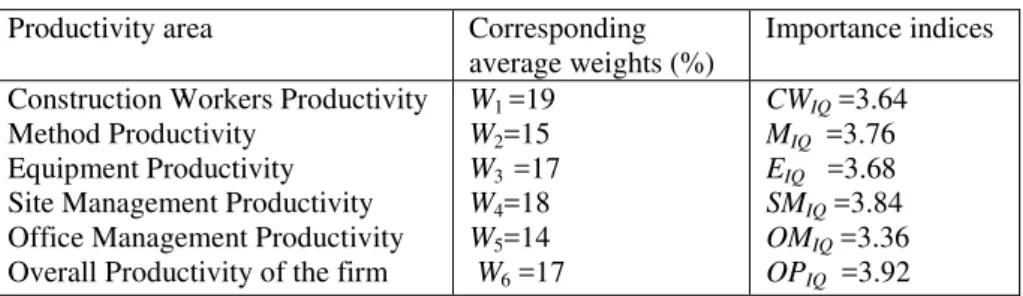
First, six productivity areas were adopted from Abu-Asba (1994) and shown in Table 1. The average of satisfaction level and average of weights of these areas will be established from a survey according to participants' point of views. Five degrees will be used, these are: extremelydissatisfied, dissatisfied, no dissatisfied no
satisfied, satisfied, and extremely satisfied. A corresponding number from 1 to 5 is assigned such that extremely dissatisfied receives 1 and extremely satisfied assigned 1. Multiplication the average of satisfaction level by the average of weights produce the denominator of productivity performance index (PPI) (see Eq. 6). The numerator of PPI is the multiplication of degree of satisfaction of productivity areas for a specific project according to actual behaviour and the previous average weights. PPI is used as the dependent variable in the predictive models of construction productivity performance.
I S P 1 I S P 2 I S P 3 I S P 4 I S P 5 I S P 6
I Q 1 I Q 2 I Q 3 I Q 4 I Q 5 I Q 6
C w W E W M W S M W O M W O P W
P P I
C w W E W M W S M W O M W O P W
(6)
Where:C w , E , M , S M , O M ,
and O P denote the productivity areas:
construction workers, equipment, methods, site management, office management, and firm's overall productivity, respectively. The subscripts, IS P and I Q express the degree of satisfaction of
productivity area for a specific project and from questionnaire, respectively. W1to W 6 are the corresponding weights of the six productivity areas obtained from survey.
Table 1: Productivity areas, corresponding average weights and importance indices
As an example for calculating PPI, assume that the importance indices (calculated from the survey) for construction workers, equipment, methods, site management, office management, and firm‟s overall productivity are: 3.25, 3.5, 3.75, 4, 3.5, 3.25 and the corresponding weights are: 0.15, 0.18, 0.2, 0.17, 0.16, 0.14, respectively. Then,
denominator of PPI
=3.25*0.15+3.5*0.18+3.75*0.2+4*0.17+3.5*0.16+ 3.25*0.14 = 3.563. Also, assume that the degree of satisfaction of productivity areas for a specific
project are : 4, 2, 3, 4, 3 and 4 for the previous areas, respectively. Then, numerator of PPI= 4*0.15+2*0.18+3*0.2+4*0.17+3* 0.16 +4 *0.14 =3.28. Accordingly, PPI=0.921 (3.28/3.563). Thus, denominator of PPI is held constant for both the equation of model developing and model validation depending on survey results, whereas, the numerator of PPI is variable according to the specific project's characteristics.
Productivity area Corresponding
average weights (%)
Importance indices
Construction Workers Productivity Method Productivity Equipment Productivity
Site Management Productivity Office Management Productivity Overall Productivity of the firm
W1 =19
W2=15
W3 =17
W4=18
W5=14
W6 =17
CWIQ =3.64
MIQ =3.76
EIQ =3.68
SMIQ =3.84
OMIQ =3.36
V.
ARTIFICIAL NEURAL NETWORK
Artificial Neural Network (ANN) is an intelligent algorithm that tries to simulate the structure or functional aspects of biological neural networks (Portas and AbouRizk, 1997; Sonmez and Rowings, 1998; Ezeldin and Sharara, 2006; Schabowicz and Hola, 2007; Hola and Schabowicz, 2010; Khan, 2012; Plebankiewicz and Le niak, 2013; Kim et al., 2014; Gerek, 2014). It consists of a large number of artificial neurons that are arranged into a sequence of layers with random connections between the layers (Tsoukalas and Uhrig, 1997).It can be arranged in different layers: input, hidden, and output. The hidden layers have no connections to the outside world because they are connected only to the input and output layers (Zayed and Halpin, 2005). The typical feed forward artificial neural network structure consists of several neurons in input layer, hidden layer and output layer where weights can be assigned to each connection between two consecutive neurons. Muqeem et al., (2011) reported that, due to strong adaptive learning and fault tolerance capabilities many researchers have used neural network as prediction model in the field of construction management.
Sonmez and Rowings (1998) and Ezeldin and Sharara (2006) employed ANN for estimating productivity of concreting works. Various neural network models have been developed for estimating labor production rates for different construction activities (Ming et al. 2000; AbouRizk et al. 2001, Moselhi et al. 2005; Song and AbouRizk, 2008). One of the applications of neural network in the engineering fields is to predict the outcome of non-linear statistical problems and is usually used to model complex relationships between inputs and outputs or to find patterns in datasets (Flores, 2011). Muqeem et al. (2011) have developed a neural network prediction model for estimating labor production rates. Tarawneh and Imam (2014) have developed Multiple Linear Regression (MLR) and ANN models for predicting pile setup for three pile types (pipe, concrete, and H-pile). It was concluded that the ANN model outperforms both the MLR model and the examined empirical formulae in predicting the measured pile setup. Kim et al. (2014) developed ANN model to estimate subgrade resilient modulus. They found that the stress state and physical properties on resilient behavior of subgrade soils were successfully correlated with the ANN model. Recently, Golizadeh et al. (2016) have developed four ANN models that trained and
tested for estimating the duration of installing
column reinforcements, installing beam
reinforcements, column concreting and beam concreting activities. Also, they designed a web-based program as an automated tool for suiting engineers to estimate the duration of scoped activities based on ANN method.
One of the most popular and efficient network structures for an ANN model is the Multilayer Perceptron (MLP) with feed forward
architecture. MLP consists of identical
interconnected neurons that are organized in layers. These layers are also connected in which outputs of one layer act as the inputs of subsequent layers. Data flow starts from the input layer and ends in the output layer. Through this journey, data pass through one or multiple hidden layers recode or provide a representation for the inputs (Flores, 2011). Thus, in the current research MLP with feed forward architecture will be adopted in developing the ANN model.
VI.
RESEARCH METHOD
Research in construction is usually carried out through experiments, case studies or surveys (Fellow and liu, 2003). Experiments on factors that affect construction productivity would take a long time to yield results, difficult to control and would therefore be expensive. Case studies would not provide results that are easy to generalize as different companies face different problems. Surveys through questionnaires were found appropriate because of the relative ease of obtaining standard data appropriate for achieving the objective of the study. Surveys are an effective means to gain a lot of data on attitudes, on issues and causal relationships and they are inexpensive to administer (Alinaitwe et al.; 2007). Accordingly, survey through questionnaires will be adopted as a research method to collect data about the
significance of factors affect construction
productivity.
VII.
QUESTIONNAIRE SURVEY
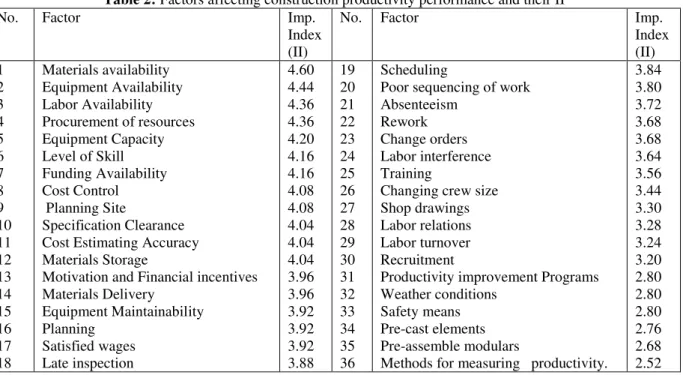
Table 2: Factors affecting construction productivity performance and their II
No. Factor Imp.
Index (II)
No. Factor Imp.
Index (II) 1 2 3 4 5 6 7 8 9 10 11 12 13 14 15 16 17 18 Materials availability Equipment Availability Labor Availability Procurement of resources Equipment Capacity Level of Skill Funding Availability Cost Control Planning Site
Specification Clearance Cost Estimating Accuracy Materials Storage
Motivation and Financial incentives Materials Delivery Equipment Maintainability Planning Satisfied wages Late inspection 4.60 4.44 4.36 4.36 4.20 4.16 4.16 4.08 4.08 4.04 4.04 4.04 3.96 3.96 3.92 3.92 3.92 3.88 19 20 21 22 23 24 25 26 27 28 29 30 31 32 33 34 35 36 Scheduling
Poor sequencing of work Absenteeism
Rework Change orders Labor interference Training
Changing crew size Shop drawings Labor relations Labor turnover Recruitment
Productivity improvement Programs Weather conditions
Safety means Pre-cast elements Pre-assemble modulars
Methods for measuring productivity.
3.84 3.80 3.72 3.68 3.68 3.64 3.56 3.44 3.30 3.28 3.24 3.20 2.80 2.80 2.80 2.76 2.68 2.52
Pilot studies were carried out to ensure the clarity and relevance of the questionnaire to contractors, also to validate and improve it. The questionnaire was shown to two researchers in the same field. One of them advocated the addition of funding availability from the clients as one of the most important factors that affect productivity performance. This factor (number 7) was added to previous factors in Table 2. A questionnaire was developed to collect data about the significance of the factors compiled in Table 2.
The participants were asked to assign a rank from 1 to 5 to each factor to represent its significance. These ranks correspond to extremely
important, very important, important, less
important, and not important, such that extremely important received 5 and not important assigned 1. Also, the participants were asked to describe their degree of satisfaction for productivity areas shown in Table 1, by marking the appropriate choice from their point of view using the previously mentioned five degrees (section 4). In addition, they were asked to identify a weight for each productivity area. Furthermore, the questionnaire included collection of data for past construction projects for the occurrence of previous factors shown in Table 2 on a yes / no basis.
VIII.
SURVEY ANALYSIS AND RESULTS
The survey gathered data from contracting companies specialized in building and civilprojects. Thirty-five contracting companies
participated in the survey. Some of the questionnaires were sent via mail after contacting
the participants through telephones, whereas, the other part was sent by some persons.
As a result of mailing and follow up a total
of twenty-five usable questionnaires were
completed and returned with a response rate, 72%
approximately. All the questionnaires were
Eq. 7, the rank is the number assigned by the respondent and it ranges from 1 to 5 according to it is significance as previously mentioned. Table 2
gives the factors rearranged in descending order according to their corresponding II.
Importance Index (II) R an k × c o rre s p o n d in g n o . o f re s p o n d e n ts T o tal n o . re s p o n d e n ts
(7)Materials availability comes out as the most important factor that affect productivity, it was received the highest II (4.6). This factor consumes a lot of contractors‟ time. Also, the main cost incurred due to shortages is for the idle time that labors have to wait for materials. Equipment availability received the second II (4.44), since some equipments are not readily available in some places even for hiring. Both labor availability and procurement of resources received an II of (4.36). Scarce of labor affect time, also, procurement of resources in a timely manner is important for the success of a project. Equipment capacity received an II of (4.2). The selection of the appropriate type and size of construction equipment often affects the required amount of time and effort and in turn the job-site productivity of a project. Both level of skill and funding availability received an II of (4.16). Level of skills seriously affects the time to accomplish tasks, the cost of labor and the quality of products achieved. Some of the respondents gave that funding availability from clients affect their cash flow and in turn affect all the project aspects: labor, materials, equipment, which affect the time, cost and quality of products achieved. Both cost control and poor site layout received the same II (4.08). Cost deviation during execution of construction projects is usually occur, thus, cost control is a mandatory requirement. Poor site layout interrupts work-flow, for example material
search difficulties, equipment transportation
difficulties or access problem. Specification clearance, estimating accuracy, materials storage received the same II (4.04). Good materials storage decreases the wastage and keeps cost of materials within the planned budget. Some of the respondents advocated that specification should be clear and explained to the executing team to avoid rework and to make the job easier. They added that bidding in large projects with many items and variables make estimating more difficult and more important to productivity. Motivation and financial incentives, and materials delivery received the same II (3.96).
It is clear that motivation and financial incentives increase the enthusiastic of labor to be more productive. The respondents declared that delivery of materials to the job site in a timely
manner is essential to keep things going and maintain high productive level.
The author suggests that factors received II equal to or higher than 4 will be considered in the predictive models. This is because factors received II equal to or higher than 4 reduce the number of variables from 36 to 12 which is a manageable number. Thus, the first 12 factors (independent variables) listed in Table 2 are used to develop the predictive models.
IX.
REGRESSION BASED MODEL
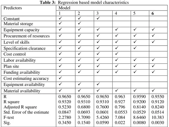
Data for 25 projects was collected and divided into two sets. The first set contains 15 projects for the purpose of model building. The second set contains 10 projects for validation purposes. SPSS 20 software was used to build the model. Enter and backward-stepping options were used. The first model in backward stepping is the same model obtained using enter method. Table 3 summarizes the results of the six models. It could be concluded that model 6 is more accurate in predicting the productivity performance index for construction projects with a higher adjusted squared multiple R=0.824 indicating that the model is able to explain 82.4% of the variability in the data, which is an excellent indicator of the model‟s expected performance. Since "adjusted R square" gives an idea of how the model generalizes, it is preferable that its value is as close as possible to the value of "R square" as in model 6 (show Table 3). On the other hand, multi-collinearity means that predictor variables are correlated with each other, making it harder to determine the role each of the correlated variables is playing. It means that the standard errors are increased. Model 6 posses the least standard error of the estimate which reflect the least multi-collinearity. Finally, because the number of projects used to build the model is 15 less than 30, F-test should be performed and the regression is significant if the sig. is less than 0.05 as in models 4, 5, and 6. Model 6 has the least sig. (0.003). As an example, the underlying formula of model 6 is PPI= 0.618 + 0.376 (equipment
capacity)+0.136(procurement of resources)
+0.145(level of skill)+0.112 (labor
(used) value. However, all the models will be validated in the section of model validation.
X.
NEURAL NETWORK BASED
MODEL
The first set contains 15 projects used in building the regression model is used here for the purpose of building the ANN model using SPSS 20
software. The Multilayer Perceptron (MLP) procedure was applied. Ten projects were used as a training set and five projects for testing set.
In this study an automatic architecture of the network was adopted to give the best architecture. Thus, three - layers ANN model with 12 neurons in the input layer of the model
Table 3: Regression based model characteristics
Predictors Model
1 2 3 4 5 6
Constant
Material storage
Equipment capacity
Procurement of resources
Level of skills
Specification clearance
Cost control
Labor availability
Plan site
Funding availability
Cost estimating accuracy
Equipment availability
Material availability
R R square
Adjusted R square Std. Error of the estimate F-test
Sig.
0.9650 0.9320 0.5230 0.0847 2.2780 0.3450
0.9650 0.9310 0.6800 0.0693 3.7090 0.1540
0.9650 0.9310 0.7600 0.0601 5.4260 0.0590
0.963 0.927 0.796 0.0553 7.084 0.022
0.9590 0.9200 0.8140 0.0529 8.6460 0.0080
0.9550 0.9120 0.8240 0.0514 10.383 0.0030
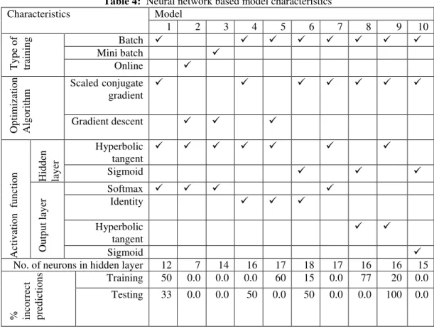
For the previously twelve factors and one output neuron for PPI were constructed. Number of neurons in the hidden layers is one of the crucial issues. Flores (2011) declared that insufficient number of neurons in the hidden layers leads to the inability of neural networks to solve the problem. On the other hand, too many neurons lead to over fitting and decreasing of network generalization capabilities due to increasing of freedom of network more than it is required. Panchal et al. (2011) and Shariati et al. (2011) explained that the best number of neurons for hidden layers depends on the number of input and output neurons, number of training cases, the complexity of learning function and training algorithm. Accordingly, ten models were tried and in all the models the automatic architecture of the network was with one hidden layer. The neurons of the hidden layer are variable according to the model developed (see Table 4).
Three types of training: batch, online and mini-batch available in SPSS 20 were adopted. Batch: updates the coefficient estimates that show
the relationship between the neurons in a given layer to the neurons in the following layer (the synaptic weights) after every single training data record. It uses information from all records in the training dataset. Online: updates the synaptic weights after every single training data record. It uses information from one record at a time. Online is superior to batch for larger datasets with associated predictors. Mini-batch: divides the training data records into groups of approximately equal size, then updates the synaptic weights after passing one group. It uses information from a group of records. However most tried cases were batch as it is preferred because it directly minimizes the total error and is useful for smaller datasets as the case here (see Table 4).
algorithms, Scaled conjugate gradient and gradient descent were tried. The activation functions: hyperbolic tangent and sigmoid were tried for the hidden layer. Also, the activation functions: identity, softmax, hyperbolic tangent and sigmoid were tried for the output layer.
All other options such as: stopping rules, maximum training time, and maximum training epochs were seated at the default. Table 4 shows
the characteristics for the ten models that have been tried. The network performance for training and testing is judged by the percentage of incorrect predictions (the relative error). However, the synaptic weights will be saved for validation purposes. An export tab was used to save the synaptic weight estimates for the dependent variable (PPI) to an XML file. These synaptic
weights will be applied to data of
Table 4: Neural network based model characteristics
Characteristics Model
1 2 3 4 5 6 7 8 9 10
T
y
p
e
o
f
tr
ain
in
g Batch
Mini batch
Online
Op
tim
izatio
n
Alg
o
rith
m
Scaled conjugate gradient
Gradient descent
Acti
v
atio
n
fu
n
ctio
n Hid
d
en
lay
er
Hyperbolic tangent
Sigmoid
Ou
tp
u
t la
y
er
Softmax
Identity
Hyperbolic tangent
Sigmoid
No. of neurons in hidden layer 12 7 14 16 17 18 17 16 16 15
% inco
rr
ec
t
p
red
ictio
n
s Training 50 0.0 0.0 0.0 60 15 0.0 77 20 0.0
Testing 33 0.0 0.0 50 0.0 50 0.0 0.0 100 0.0
Holdout set (the second set which contains 10 projects) for validation purposes. All these models will be validated in the section of model validation.
XI.
MODELS VALIDATION
The other 10 projects excluded during models development were used for validation purpose. All the models were used to produce 10 predicted values for the PPI of the 10 projects. The results of models validation are shown in Table 5. The following subsections describe the validation process for both regression based models and neural network based models.
11.1. Regression Based Models
As an example for models validation, model 6 used in predicting PPI for all projects (see Table 5). For example project 8 with the following
characteristics: equipments capacity was
satisfactory (1); the resources were procured in a timely manner (1); level of skill was satisfactory (1); the labors were available (1); the site was poorly planned (0); funds were available (1); the materials were available (1). The predicted PPI will be obtained as follows:
PPI= 0.618 - 0.376*1 + 0.136*1 + 0.145*1+0.112*1 +0.168*0 - 0.119* 1- 0.353*1=0.915=91.5%
This result means that this project is expected to have a poor performance equal to
the actual values of PPI (APPI) and the predicted values of PPI (PPPI). Golizaadeh et al. (2016) reported that best performance of the model is measured based on the error produced by the model, which is the Mean Absolute Percentage Error (MAPE). MAPE expresses accuracy as a percentage and is defined by Eq. (8). The absolute percentage errors for each project in model 6 are
shown for example, whereas MAPE for all models are shown in ascending order. It is clear that model 6 is the best model because it received the least MAPE (19.21%). In addition, model 6 posses the best characteristics of adjusted R square, least standard error of the estimate, and accepted sig. limits.
n
i i
n 1 i
1 A P P I P P P I
M A P E 1 0 0
n A P P I
(8)Table 5: Models Validation
Regression based model Neural network based model
Proj. Model 6 MAPE for
each model
Model 4 MAPE for
each model
APPI PPPI % error* Model value APPI PPPI % error* Model value
1 0.884 1.083 22.51 6 19.21 0.884 0.99 11.99 4 12.49
2 1.137 0.915 19.53 4 19.47 1.137 1.08 5.01 7 12.69
3 1.049 1.043 0.57 5 19.72 1.049 0.95 9.44 8 12.85
4 0.951 1.3 36.69 1 20.49 0.951 0.95 0.42 3 12.86
5 0.757 1.057 39.63 2 22.62 0.757 0.98 29.46 2 12.94
6 1.078 1.202 11.50 3 23.64 1.078 1.08 0.19 10 13.03
7 0.943 0.618 34.46 0.943 0.81 14.1 5 13.08
8 0.859 0.915 6.52 0.859 1.16 35.04 1 13.42
9 1.124 1.083 3.65 1.124 0.95 15.48 9 13.79
10 0.987 1.155 17.02 0.987 0.95 3.75 6 15.27
*= i i
i A P P I P P P I
A P P I
11.2 Artificial Neural Network Based Models
The ten projects included in the holdout set were validated using scoring wizard from utilities menu in SPSS 20. Ten models were tried as shown in Table 6. Different types of training, optimization algorithms, and activation functions for hidden and output layers were adopted. The synaptic weights were applied to data of holdout set for determining PPPI. PPPI for each project in model 4 is given for example and the absolute
percentage error between PPPI and APPI (see Table 5). Also, MAPE is shown in Table 5 for all models in ascending order. Out of the ten models tried, model 4 with batch training, scaled conjugate gradient as optimization algorithm and hyperbolic tangent and identity activation functions for input and output layers, respectively is the best model (MAPE;12.49%). Fig. 1 shows the schematic architecture of model 4.
XII.
SUMMARY AND CONCLUSIONS
This paper investigated the effect ofqualitative factors affecting productivity of
construction firms through a questionnaire survey. These factors were established from literature. A standard methodology was adopted. First, a single quantifiable measure, a productivity performance index (PPI) was developed to measure the productivity performance of the surveyed projects and was considered the dependent variable in the developed models based on regression and neural networks. Neural networks in literature were then presented. Questionnaire survey was then prepared and the results were analyzed.
Based on the results of the questionnaires an importance index was established for each factor to quantify its effect on construction productivity performance. It was intended that factors received an importance index equal to or higher than 4 are significant and will be incorporated into the model
as independent variables. Accordingly, 12
significant variables were identified.
Two types of models based on regression analysis and neural networks were developed to predict PPI. In regression analysis based models enter and backward- stepping techniques were applied resulting in six models. Ten models based on neural networks were tried using Multilayer Perceptron with different characteristics.
Validation of the proposed models revealed that out of ten models tried by neural networks, the model with batch training, scaled conjugate gradient as optimization algorithm and hyperbolic tangent and identity activation functions for input and output layers, respectively was the best model tried from all models tried by regression analysis and neural networks. This model gave Mean Average Percentage Error between the actual values of PPI and its predicted values by approximately 12.5%, whereas this percentage is 19.2% for the best model obtained based on regression analysis.
This research is relevant to both industry practitioners and researchers. It provides a systematic approach for practitioners to predict productivity performance for construction firms. In
addition, it provides researchers with a
methodology to build regression based models and neural network based models suitable for productivity performance. However, according to the dynamic nature of construction industry the author hopes that in future other factors will be investigated to quantify their effect on productivity performance. Also, other techniques will be applied in prediction such as: Statistical-Fuzzy Approach.
REFERENCES
[1]. Abdel-Razek, R., H., Hany, M., A., and
Abdel Hamid, M. (2007)." Labor
productivity: benchmarking and variability in Egyptian projects." Int. J. Proj. Manage. 25 (2), 189-197.
[2]. AbouRizk, S., Knowles, P. and Hermann, U.R. (2001).“Estimating labor production rates for industrial construction activities” J. Constr. Eng. Manage., Vol. 127, No. 6, ASCE, ISSN 0733- 9634/01/0006-0502– 0511.
[3]. Abu-Asba, M.M. (1994). “Construction
productivity awareness and improvement programs in Saudi Arabia.” Ms.c Thesis, King Fahd Univ. of Petroleum & Minerals, Dhahran, Saudi Arabia.
[4]. Alinaitwe, H. M., Mwakali, J. A., and Hansson, B. (2007).“Factors affecting the productivity of building craftsmen-studies of Uganda.” J. of Civ. Eng. and Manage.
[5]. Charamokos, J., and Mc Kee, K.E. (1981).
“Construction productivity improvement.” J. of Constr. Division, ASCE, 107 (1), 35-47.
[6]. Choy, C. F. (2009). “Productive efficiency
of Malaysian construction sector.” Faculty of Eng. and Sci., Univ. Tunku Abdul Rahman, Malaysia.
[7]. Ezeldin, A. S. and Sharara, L. M. (2006). “Neural networks for estimating the productivity of concreting activities.” J. Constr. Eng. Manage., Vol. 132, No. 6, 650-656, DOI: 10.1061/(ASCE) 0733-9364.
[8]. Fellows, R. and Liu, A. (2003). “Research
methods for construction.” 2nd ed., Blackwell Science, Oxford.
[9]. Flores, J. A. (2011). "Focus on artificial
neural networks." Nova Science
Publishers.
[10]. Gerek, I. H. (2014). “House selling price assessment using two different adaptive neuro-fuzzy techniques.” Automation in
Constr., Vol. 41, 33-39, DOI:
10.1016/j.autcon.
[11]. Giovannini, E. and Nezu, R.
(2001)."Measuring productivity:
measurement of aggregate and
industry-level productivity growth." OECD
Publications, 2, rue André-Pascal, 75775 Paris Cedex 16, France.
[12]. Golizadeh, H., Sadeghifam, A.N., Aadal,
h., and abd Majid, M.,
Vol. 20, No.1,12-22, DOI 10.1007/s12205-015-0263- 12.
[13]. Hiyassat, M.A., Hiyari, M.A., and Sweis, G.J. (2016) "Factors affecting construction labour productivity: a case study of Jordan." Int. J. Constr. Manage., Vol. 16,
No.2, 138-149, DOI:
10.1080/15623599.2016.1142266.
[14]. Hola, B. and Schabowicz, K. (2010).
“Estimation of earthworks execution time cost by means of artificial neural networks.” Automation in Constr., Vol.
19, No. 3, 570-579, DOI:
10.1016/j.autcon.
[15]. Hola, B. and Schabowicz, K. (2010).
“Estimation of earthworks execution time cost by means of artificial neural networks.” Automation in Constr., Vol. 19, No. 3, 570-579.
[16]. Hope, J. and Hope, T. (1997).“Competing
in the third wave: the teen key management issues of the information age.” Boston, Harvard Business School Press.
[17]. http://www.sussex.ac.uk/its/pdfs/SPSS_N
eural_Network_22.pdf [18]. https://spss-64bits.jaleco.com/
[19]. Ibbs, W., and Liu, M.(2005)." Improved measured mile analysis technique." J. Constr. Eng. Manage., ASCE, 131 (12), 2005.
[20]. Idiake, J., E., and Bustani, S. A. (2014). "Relationship between labour performance and variability in block work workflow and labour productivity." Civ. Environ. Research www.iiste.org, Vol.6, No.2.
[21]. Kaming, P. F., Holt, G. D., Kometa, S.T.,
and Olomolaiye, P. (1998). “Severity diagnosis of productivity problems: a reliability analysis.” Int. J. Proj. Manage., 16 (2), 107-113.
[22]. Karmale, S., and Biswas, A. P. (2015)." Improving labor productivity on building construction projects." Int. J. Eng. Science & Research Technology, 4(6), 828-832. [23]. Khan, M. I. (2012). “Predicting properties
of high performance concrete containing composite cementitious materials using artificial neural Networks.” Automation in Constr., Vol. 22, 516-524.
[24]. Kim, S. H., Yang, J., and Jeong, J. H. (2014). “Prediction of subgrade resilient modulus using artificial neural network.” KSCE J. Civ. Eng., Vol. 18, No. 5, 1372-1379, DOI: 10.1007/ s12205-014-0316-6.
[25]. Kohn, E., and Caplan, S.B. (1987). “Work
Improvement Data for Small and Medium
Size Contractors.” J. Constr. Eng. and Manage., ASCE, 113 (2), 327-339.
[26]. Lema, M. N. (1996). “Construction labour
productivity analysis and benchmarking – the case of Tanzania.” PhD thesis, Loughborough Uni., UK.
[27]. Lim, E. C., and Alum, J. (1995).
“Construction productivity: issues encountered by contractors in Singapore.” Int. J. of Proj. Manage., 13(1), 51-58. [28]. Lin, C. and Huang, H. (2010). "Improved
baseline productivity analysis technique." J. Constr. Eng. Manage., 136(3), 367–376. [29]. Liu, M., Ballard, G., and Ibbs, W. (2011)."
Work flow variation and labor
productivity: case study." J. Manage. Eng., Vol. 27, No. 4, 236-242.
[30]. Makulsawatudom, A. and Emsley, M.
(2002). “Critical factors influencing
construction productivity in Thailand.” Proc. Of CIB 10 th Intern. Symposium
Constr. Innovation and Global
Competitiveness, Cincinnati, Ohia, USA, 9-13.
[31]. Ming, L., AbouRizk, S.M., and Herman,
U. (2000). “Estimating construction
productivity using probability inference neural network” J. of Computing in Civ. Eng., Vol. 14, No. 4, ASCE, ISSN 0887-3801/00/0004-0241–0248.
[32]. Mosehli, O., Assem, I. and El- Rayes, K. (2005). “Change order impact on labor productivity” J. of Constr. Eng. and Manage., Vol. 131, No. 3, 354–359. [33]. Motwani, J., Kumar, A. and Novakoski,
M. (1995). “Measuring construction
productivity: a practical approach.” Work study, 44(8), 18-20.
[34]. Muqeem, S., Idrus, A. B., Khamidi, M. F.,
and Zakaria, S. B.(2011) " Prediction modeling of construction labor production rates using artificial neural network" Proceeding of 2nd Int. Conference on Environ. Sci. and Tech., Vol 6, Singapore.
[35]. Olomolaiye, P., Wahab, K., and Prince, A.
(1987). “Problems influencing craftsmen productivity in Nigeria.” J. of Building and Environ., 22 (4), 317- 323.
[36]. Mosehli, O., Assem, I., and El- Rayes, K.,
(2005) “Change order impact on labor
productivity” J. Constr. Eng. Manage., Vol. 131, No. 3,ASCE, ISSN 0733-9364. [37]. Panchal, G., Ganatra, A., Kosta, Y., and
of Computer Theory and Eng., Vol. 3, 332-337.
[38]. Plebankiewicz, E. and Leoeniak, A.
(2013). “Overhead costs and profit calculation by Polish contractors.”
Technological and Economic
Development of Economy, Vol. 19, No. 1, 141-161.
[39]. Portas, J. and AbouRizk, S. (1997).
“Neural network model for estimating construction productivity.” J. Constr. Eng. Manage., Vol. 123, No. 4, 399-410, DOI: 10.1061/ (ASCE)0733- 9364.
[40]. Sonmez, R. (1996). “Construction labor
productivity modeling with neural
network and regression analysis" Graduate thesis submitted for the degree of Doctor of Philosophy Lowa State University.
[41]. Schabowicz, K. and Hola, B. (2007).
“Mathematical-neural model for assessing productivity of earthmoving machinery.” J. Civ. Eng. Manage. , Vol. 13, 47-54.
[42]. Shariati, O., Zin, A. M., and
Aghamohammadi, M. (2011). Application of neural network observer for on-line estimation of salient-pole synchronous generators‟ dynamic parameters using the operating data." In Modeling, Simulation and Applied Optimization (ICMSAO), 4th
International Conference,1-9, IEEE,
10.1109/ ICMSAO.2011.5775505. [43]. Song, L. and AbouRizk, S.M. (2008).
“Measuring and modelling labor productivity using historical data” J. Constr. Eng. Manage., Vol. 134, No. 10. [44]. Sonmez, R. and Rowings, J. E. (1998).
“Construction labor productivity modeling with neural networks.” ” J. Constr. Eng. Manage., Vol. 124, No. 6, 498-504, DOI: 10.1061/ (ASCE)0733-9364.
[45]. Strandell, M. (1978). “Productivity in the construction industry.” AACE Bulletin, 20 (2), 57-61.
[46]. Strandell, M., (1982). “Understanding the word “Productivity” What it means and what is behind it? AACE Transaction, G.1.1-G.1.3.
[47]. Tarawneh, B. and Imam, R. (2014).
“Regression versus artificial neural networks: predicting pile setup from empirical data.” KSCE Journal of Civil Engineering, Vol. 18, No. 4, 1018-1027, DOI: 10.1007/ s12205-014-0072-7.
[48]. The Business Roundtable, (1982).
“Measuring productivity in construction.”
Report A-1, Constr. Industry Cost
Effectiveness Project, New York, N.Y.
[49]. Thomas, A., V. and Sudhakumar, J.
(2013)." Labour productivity variability among labour force – A case study." The International Journal of Engineering And Science, Volume 2, 5, 57-65.
[50]. Tsoukalas, L.H, and Uhrig, R.E. (1997). “Fuzzy and neural approaches in engineering”, Wiley, New York.
[51]. Zakeri, M., Olomolaiye, P., Holt, G., and
Harris, F.C., (1996). “A survey of
constraints on iranian construction
operatives‟ productivity.” Constr. Manage. and Economics, 14 (5), 417-426.
[52]. Zayed, T.M., and Halpin, D. W.,(2005)."
Pile construction productivity