Workplace Diversity and Incentive Contracts:
Theory and Evidence
Daniel Ferreira
∗November 27, 2001 (Job Market Paper)
Abstract
This paper presents a simple theory of the provision of incentives infirms in which the principal optimally chooses both compensation contracts and the composition of the work force. Assuming that individuals display group loyalty, a less diverse (more homogeneous) work force will be more cooperative. Simple comparative statics provide some testable implications relating risk, diversity and incentive pay. I also analyze the case in which workers’ characteristics cannot be readily observed ex ante. The theory then predicts that firms are more likely to prevent workers from interacting with each other when workers are expected to have similar characteristics. This shows a surprising effect of diversity in the workplace: more diverse firms will promote more interactions between workers of different types, i.e. they will be less segregated.
I test the main predictions of the model using a cross-sectional sample of corporate boards. I use the proportion of women on boards as a measure of diversity. There are three main empiricalfindings: (1) a significant negative correlation betweenfirm risk and diversity, (2) a significant positive relation-ship between performance-based compensation and diversity and (3) a significant positive correlation between the number of board meetings (a measure of interactions among directors) and diversity. The evidence is broadly consistent with the implications of the theory.
∗Ph. D. Candidate, Department of Economics, The University of Chicago. E-mail: [email protected]. This is a
condensed version of my Ph. D. dissertation and my job market paper. Some extensions of this work are in the appendices that can be downloaded from http://home.uchicago.edu/~dsferrei. I am especially grateful to Canice Prendergast, Raaj K. Sah, Pierre-André Chiappori and Luis Garicano for their help and guidance in the process of writing this paper. I am also thankful to Bernard Salanié, who carefully read a very preliminary version of this paper and pointed out many ways of improving it. I also benefited from comments by Luis Braido, Carlos da Costa, Maitreesh Ghatak, Hugo Sonnenschein and Andrea Tiseno. Finally, I am very grateful to Renée Adams for many discussions on this topic and also for helping me with the data. The usual disclaimer applies.
1
Introduction
Firms are social institutions, where workers with possibly different personal characteristics and back-grounds interact with each other. An economically interesting question arises when social interactions
in the workplace change workers’ responses to the incentive structure imposed by firms. This paper
analyzes the effects of group loyalty, or the tendency to care about the well-being of people who have characteristics that are similar to one’s own, on the provision of incentives in firms. I present a model in
which a principal can use three different instruments to induce effort from her workers: incentive pay, the composition of the work force (i.e., its degree of diversity) and the amount of social interactions among
workers in the workplace. The model predicts certain relationships among these three instruments. I test
the main implications of the theory using data on directors of publicly traded corporations. The empirical
results provide some preliminary but surprisingly strong support for the theory. The evidence suggests
that there are gains to incorporating variables such as diversity and social interactions into formal models
of incentives in organizations. This paper is a first step in that direction. I show that introducing the
ideas of group loyalty, diversity and social interactions in an otherwise standard principal-agent model
generates new implications and suggests different ways of looking at data.
Group loyalty may be a consequence of identification, or the feeling of being part of a group.1
This paper adopts the assumption that increasing the diversity of the work force reduces its group
loyalty. This relationship between similarity and attraction is well documented in the social psychology
literature (Byrne, 1969; Lott and Lott, 1965; Zander, 1979). Although groups are usually associated with
characteristics such as race and gender, other characteristics may well lead to group loyalty. Therefore,
I interpret diversity broadly. I assume that employees can be characterized by their types. As in Athey
et al. (2000), “(types) can be interpreted as gender, ethnicity, cultural background, personality type,
or even skill set (e.g., operations versus marketing skills for managers, theorists versus empiricists for
academics)” (p.765).
I develop a simple model in which one principal (firm) needs to employ two agents (a team of workers)
to produce one single output. Effort is not observable, therefore the usual moral hazard problems arise.
1 Simon (1991) suggests that identification with an organization is a way of reducing agency problems. See also Akerlof
The principal can design a compensation contract that links workers’ pay to team performance. However,
incentive pay is costly due to workers’ risk-aversion. The principal can also choose the composition of
the team, based on her knowledge of workers’ characteristics. The degree of similarity between workers
will affect their degree of group loyalty. Therefore, a more homogeneous (less diverse) team is more cooperative and exerts more effort than a less homogeneous (more diverse) one. Thus, the principal prefers homogeneous teams. However, choosing a very homogeneous work force might also be costly.
Finding people with very similar characteristics demands time and resources. This cost should increase
with the degree of desired similarity, because no two people are exactly alike.2 The principal’s problem
is to find the optimal combination of these two instruments.
A natural question that arises in this context is whether work force homogeneity and incentive pay are
substitutes or complements. Common intuition suggests that they are substitutes: if incentive pay is very
costly, the firm may want to rely more on work force homogeneity as a means of providing incentives,
and vice-versa.3 However, my model shows that homogeneity and incentive pay can sometimes be
complements. Work force homogeneity increases the total levels of effort for a given incentive scheme. Therefore, more homogeneity makes workers more sensitive to monetary incentives, which may lead to
complementarities between the two instruments.
Although this ambiguity might suggest that the implications of the model are not easily testable, this is
not true. The main testable implication is thatincentive pay and work force homogeneity are two different
instruments to achieve a common goal. If they are complements, incentive pay is positively related to
homogeneity while risk (the cost of providing incentive pay) should be negatively related to homogeneity.
If they are substitutes, incentive pay is negatively related to homogeneity while risk (the cost of providing
incentive pay) should be positively related to homogeneity. In other words, the relationship between risk
and homogeneity should have the opposite sign as the relationship between homogeneity and incentive pay.
This a clear-cut empirical prediction, one that the evidence I present in this paper is consistent with.
When I introduce uncertainty about workers’ personal characteristics,firms gain a third instrument
to induce effort from workers. As long as some workers’ characteristics cannot be perfectly observed ex ante, workers will gradually learn about coworkers’ characteristics if meeting and talking to each
other is required by the nature of their jobs. Firms may want to organize work in ways that promote
2
Homogeneity costs may be either exogenous, such as search costs or opportunity costs for not hiring workers based on their productive characteristics, or endogenous costs, such as the ones arising from excessive conformity or the increasing likelihood of collusion among workers.
or prevent this kind of learning. In short, the amount of interactions among workers in the workplace
is also a variable that is at least partially under the principal’s control. I show that firms will distort
the organization of work in order to facilitate learning when workers are expected to be different from each other. When workers are expected to be similar, firms prefer to restrict social interactions in the
workplace in order to prevent learning.
This result shows that policies towards more diversity infirms may have some surprising consequences.
If differences in observable and unobservable characteristics are not too negatively correlated, policies (like affirmative action) that requirefirms to hire a diverse work force in terms of observable characteristics may lead them to promote social interactions in the workplace in order to improve learning about workers’
unobservable characteristics. In short, more diverse firms will also be less segregated: employees of
different types will interact more than employees of similar types. The intuition behind this result is that, when workers hold negative stereotypes about coworkers, cooperation is initially very low, therefore
firms do not have much to lose if negative stereotypes are confirmed ex post, but they do gain a lot if
learning reveals that stereotypes were not justified. This implication is also testable: diversity should be
positively related to the amount of interactions among workers in the workplace.
In the empirical part of this paper, I look at a cross-sectional sample of boards of directors of 1462
publicly traded firms in fiscal year 1998. Boards are good examples of teams and their members are
offered the same compensation contracts. Because information on directors is usually available to the public (due to regulations, listing requirements or shareholder activism), measures of diversity can be
constructed using demographic information on individual directors. In this paper I use the proportion of
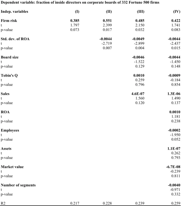
women on boards as a measure of diversity, but I also briefly discuss the distinction between inside and
outside directors as an alternative measure of diversity.4
The empirical evidence provides strong support for the hypothesis that proportions of men and women
affect the design of compensation contracts and thatfirms take that into account when choosing the gender composition of their work force. I cannot empirically reject the two main implications of the model. I
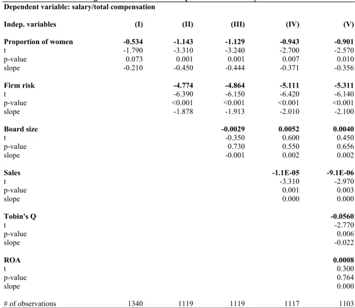
find diversity to be negatively related tofirm risk and positively related to incentive pay, which confirms
thefirst prediction. Incidently, this evidence also suggests that work force homogeneity and incentive pay
are indeed substitutes, in accordance with simple intuition. I also find that directors meet more often in
more diverse firms, which confirms the second prediction.
4 I chose these measures of diversity mainly because they are relatively easy to collect. I plan to extend the analysis in
I find that firms facing more variability in their stock returns have fewer women on their boards of
directors. This result is surprisingly strong and very robust. The model fits the evidence better than
other competing explanations, such as claims that women are less efficient in complex environments, that women are more “stabilizing” or that women are more risk-averse. In my model, a negative relationship
between diversity and firm risk implies that incentive pay and work force homogeneity are substitutes.
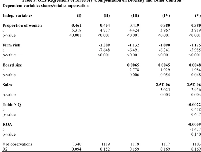
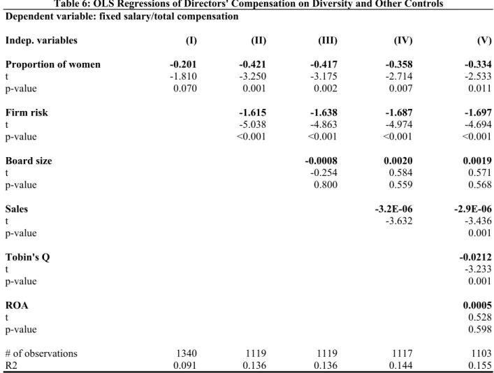
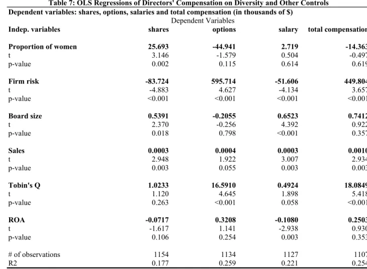
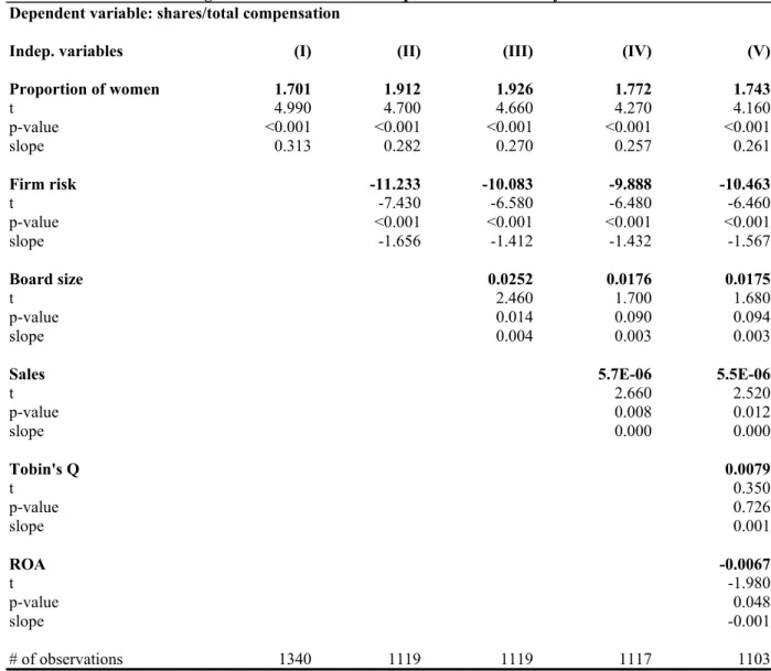
Therefore, after controlling for risk, incentive pay should be positively related to diversity. Consistent
with this implication, I find that restricted stock comprises a greater share of director compensation in
firms with relatively more women on their boards. Thisfinding is also robust. Together, these two pieces
of evidence suggest that incentive pay and work force homogeneity are substitutes.
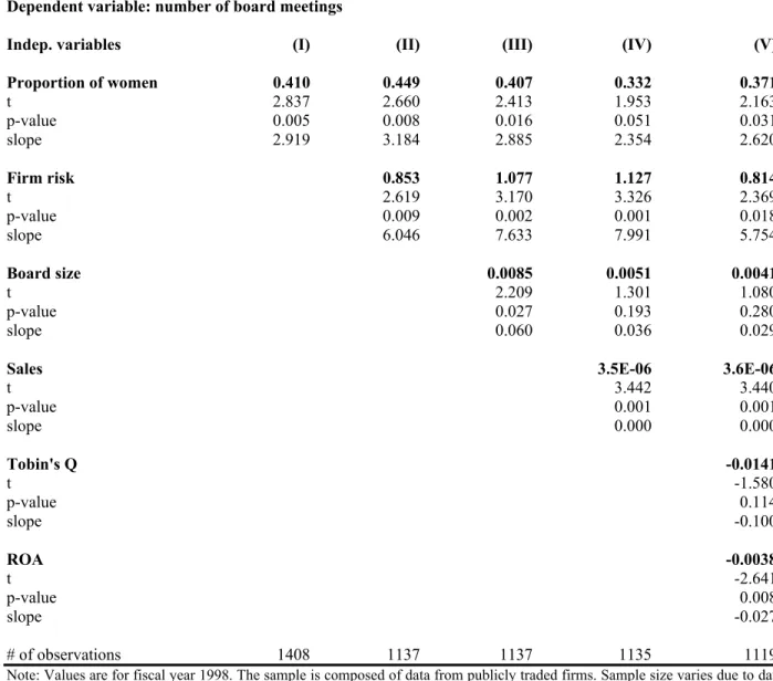
I use the number of board meetings as a proxy for social interactions among directors in the workplace.
Consistent with the theory, I find a positive correlation between the number of board meetings and
diversity. Therefore, the main implications of the model survive empirical scrutiny.
To my knowledge, this is thefirst paper that studies the relationship between work force composition
and the provision of incentives in firms.5 In this paper, as in Kandel and Lazear (1992) and Rotemberg
(1994), I analyze the effects of social relations among workers on their incentives to cooperate. However, unlike them I assume a principal-agent relationship between a manager and a team of workers. This allows
me to study the relationship between the design of incentive contracts and the organization of work. My
model assumes that workers may be altruistic towards coworkers, as in Rotemberg (1994).6 Altruism
can be either positive or negative. I assume that the main determinant of altruism is the difference in workers’ personal characteristics, i.e. altruism is a function of group loyalty. This is how diversity
affects the willingness to cooperate. Group-based incentives have distorted effects when preferences are interdependent, which is the case here. Therefore, workplace diversity and incentive contracts are closely
connected.
The paper is organized as follows. In section 2, I describe a model with two agents and one principal,
5 Few papers have looked at some related issues. Kandel and Lazear (1992) showed how some nonpecuniary motives,
like peer pressure, can improve efficiency in partnerships. Rotemberg (1994) modeled the acquisition of altruism among workers and showed how it increases incentives to cooperate. Both papers claim that partnerships provide incentives for workers to internalize nonpecuniary motives to cooperate. Peer pressure and altruism arise endogenously in their models. However, they limited their analyses to the study of partnerships, leaving aside the agency problems that might arise when teams work for a principal. Prendergast and Topel (1996) analyzed the design of compensation contracts and work practices under the assumption that supervisors are subject to favoritism bias; i.e., supervisors may “like” or “dislike” some of their subordinates. They explicitly work with a principal-agent framework, but, unlike Kandel and Lazear (1992) and Rotemberg (1994), they focus on relations between managers and workers, instead of social relations among workers.
6
in which agents’ utilities are interdependent, and in which preference interdependency is affected by how similar agents are. In section 3, I characterize the optimal contract assuming that workers’ characteristics
can be observed and discuss its main properties. In section 4, I introduce unobserved characteristics into
the model and then discuss the incentives for the principal to promote or prevent learning in the workplace.
Section 5 describes the data. I discuss the empirical findings in section 6. Section 7 concludes.
2
A Model of Group Loyalty
2.1
Similarity
Consider two workersiandj.Letvi andvj be their respectivetypes. Types could have many dimensions,
some that can be easily observed, like race and gender, and some others that cannot be so easily observed,
like religion and political orientation. I assume the existence of a variable which I callsimilarity. Similarity
is a function of types:
γ=γ(vi, vj) (1)
The idea is that a highγ implies that the two agents have characteristics that are in some sense “close”
to each other’s. I assume that γis a number on the real line.
Let the loyalty parameter αi represent a measure of how much agent i cares for agent j ’s utility,
i.e. it is a measure of altruism.7 What determines αi? I assume that individuals differ in (possibly unobservable) characteristics and that those characteristics affect how much they care for each other’s well-being. More specifically, let us assume that individuals in a population have different characteristics (or types) and that they have a preference for interacting with people that have characteristics that are
similar to their own. For example, in a population of Democrats and Republicans, when two persons
are randomly matched, a Democrat (Republican) will become more altruistic towards her match if she
learns that this person is also a Democrat (Republican). But learning that the other person is of an
undesirable type may decrease altruism, which could even be negative (e.g., hatred or envy). The group
loyalty assumption is then equivalent to assuming thatαi is an increasing function ofγ.
However, from agenti’s viewpoint,γmay be a random variable, since she may not know the value of
vj for sure. In an ex ante sense, similarity is a random variable whose distribution is determined by the
distribution of types in the population. To simplify the problem, I assume that agent ionly cares about
7 I will explain below the precise relationship betweenα
expected similarity. Therefore, the loyalty parameter is given by
αi=E[γ(vi, vj)|Ii] (2)
where Ii is agent i’s information set.8
In section 3, I assume that types are known with certainty before contracts are offered and actions are taken, therefore loyalty parameters can be considered exogenous variables. Later I introduce uncertainty
about types and then loyalty parameters might be seen as endogenous variables, which depend on how
often workers interact and learn about each other’s types.
2.2
Technology
A manager (principal) needs exactly two specialized workers (agents) in order to generate profits. It is
assumed for simplicity that the manager herself does not have the specific human capital to become a
worker. When workers are matched with the manager, they generate revenues that are positively related
to their privately chosen effort levels. Output (or revenue)x is given by:
x=e1+e2+ε (3)
where ei is the effort level chosen by workeriand εvN(0,σ2).
The assumption of pure team production (i.e., no individual signal of performance) is made for
simplicity. Team production creates free-riding problems, on top of usual moral hazard problems of
single-agent settings. I show that diversity worsens free-riding problems because agents become less
cooperative when group loyalty (altruism) is low. Therefore, at least some amount of joint production is
required for the analysis that follows.
It should be emphasized, however, that what is required here is that optimal contracts be designed
in a way that makes compensation of individual workers dependent on the actions taken by all workers.
In Mookherjee’s (1984) more general analysis of multi-agency problems, individual pay often depends on
actions taken by other agents. Furthermore, under interpersonal preferences, there is a natural incentive
to adopt technologies and to design tasks such that individual inputs are complements. Therefore, instead
of being assumed, teamwork could arise endogenously as in Itoh (1991).9
8 I relax this assumption in Appendix C. One can download the appendices from
http://home.uchicago.edu/~dsferrei/appendix.pdf
9
free-The timing of the game is as follows. In period 0, the manager chooses two workers based on their
observed characteristics. In the beginning of period 1, the manager offers a take-it-or-leave-it wage schedule (w1, w2) to both workers. Workers can either reject the offers (and get outside utility of U0) or
accept them. If they accept the offers, workers simultaneously and non-cooperatively choose their effort levels(e1, e2).Then the manager observesx, which is a noisy signal of the aggregate effort level, and then
pays wages and collects profits.
2.3
Preferences
The manager is risk neutral, i.e. her utility function is given by
V =E[x−w1(x)−w2(x)] (4)
Wages will usually be functions of observed output.
Workers are risk-averse and may be altruistic. I assume that workeri’s “egoistic” utility is given by
ui=−exp{−r[wi(x)−C(ei)]} (5)
where r is the (constant) absolute risk aversion coefficient and C(ei) is the cost of effort. When worker
iis altruistic, (5) represents the utility that she derives from her own consumption and effort. Following Stark (1995), I call this function worker i’s “felicity”.
Workeri’s total utility is given by
Ui =ui(−uj)αi (6)
The loyalty (or altruism) parameter αi represents the weight that worker igives workerj’s felicity.
The utility in (6) is analogous to standard utility functions found in the altruism literature, except for
the fact that the other worker’s utility enters multiplicatively instead of additively.10 I chose this form in
order to preserve the exponential nature of the utility function, which simplifies the computation of the
optimal contract. As I show below, this formulation is equivalent to assuming that certainty equivalents
are linear functions of each other.
riding problems. This literature usually cites many reasons why teams could increase productive efficiency: they foster participation, communication and cooperation among workers, they increase their sense of responsibility, promote a better work environment, and so on. For examples, see Cohen and Bailey (1997), Cohen and Ledford (1994), Dunphy and Bryant (1996) and Hackman (1990).
1 0
Assuming this type of altruistic utility function amounts to assuming that agents are willing to sacrifice
some of their own “utility” to increase the utility of the other agent. This is one (but not the only) way
to generate the type of taste-based cooperation I am concerned with in this paper.11
Since the results I derive in this paper crucially depend on the specification of preferences, I want to
stress three points regarding the utility in (6).
First, one could have chosen a different specification of altruism in which agent i’s total utility is a function of her own felicity and of agentj’s total utility. It turns out that utilities like the one in (6) can
be seen as reduced-form solutions of a system of “structural” utilities like:
Ui=−(−ui)βi[−Uj]ηi (7)
where i, j = 1,2 (see Stark, 1995). Therefore, I start directly from (6) for simplicity and to save on
unnecessary notation.
Second, it might seem natural to restrict the range ofαi.A natural restriction is to imposeαi ≤1.This
simply assumes that agents value their own consumption no less than they value others’ consumption.12
Some may also want to rule out hatred or envy, i.e. to impose αi ≥ 0. It turns out that, in the
model I develop in this paper, it is more convenient to assume that αi has an unrestricted range, i.e.
αi ∈ (−∞,∞). All but the last result in this paper do not depend on this assumption, therefore they
are still valid if any of the above restrictions are imposed. I will show that, under weak assumptions,
αi will never be negative in equilibrium. Also, one may think of very high or very low values of αi as
being possible but very hard tofind in a given population (in other words, they are events with very low
probability).
Third, in utility (6), altruism αi has level effects: if a person becomes more altruistic, she becomes
“happier”. In other words, altruism is a good. A different altruistic utility function that does not display this property is:
Ui=−[−ui]
1
1+α[−uj] α
1+α (8)
It turns out that the results in this paper are the same with or without level effects. Therefore, the discussion about which one of (6) or (8) is more realistic is largely irrelevant for my results.
1 1 Other ways include assuming that workers derive utility from the act of cooperating or that workers are driven by
reciprocity considerations. For a recent model in which agents derive utility from cooperation, see Rob and Zemsky (2000). For experimental evidence of reciprocity considerations in contract enforcement, see Fehr, Gatcher and Kirschsteiger (1997).
1 2
2.4
Some Benchmark Cases
For the benchmark cases, I will assume that workers are egoistic (i.e., αi = αj = 0). I will also assume
from now on that the cost of effort is given byC(ei) = k2e 2 i.
With exponential utilities and normally distributed errors, Holmstrom and Milgrom (1987)
rational-ized the use of linear contracts like wi(x) = aix+bi .13 Furthermore, since the only observable (and
verifiable) variable isx, wage schedules can depend only onx. Because both workers are ex ante identical
in all aspects, it will never be optimal to treat workers differently, so I will focus only on the cases in which w1 =w2=w. The outside utility isU0 =−exp{−rw0}.
2.4.1 The First-Best
The first-best contract is the one in which both workers’ efforts are perfectly observable and verifiable (the same outcome could also be implemented as a Nash equilibrium if the principal could only observe
the sum of workers’ efforts, since she could act as a budget breaker. See Holmstrom (1982)). The first-best levels of effort are eF B1 = eF B2 =
1
k, while wages are constant w
F B = 1
2k+w0 and profits are
VF B = 1k−2w0.
2.4.2 The “No-Cooperation” Contract
I call the “no-cooperation” contract the solution to the problem in which the manager can only observex,
which is a noisy measure of the aggregate level of effort, and workers simultaneously and non-cooperatively choose their effort levels. Considering a linear contract like w(x) =ax+b, the optimal contract is14
aN C = 1 1 +kc, e
N C = 1
k(1 +kc), b
N C = 1
2
kc−3
k(1 +kc)2 +w0, V
N C = 1
k(1 +kc)+ 2w0 (9)
Simple algebra shows that VF B > VN C and eF B > e N C; i.e., both effort levels and profits mono-tonically decrease from the first-best to the no-cooperation solution.
1 3
Formally, Holmstrom and Milgrom (1987) assumed that the agent chooses efforts continuously over the time interval [0,1]to affect the drift of a Brownian motion. They show then that the agent would choose a time-invariant effort level and that the optimal contract is linear in thefinal outputx.Therefore, the one-shot linear-contracts version of this problem will give us the same answer as its continuous-time version.
1 4 This case is a relatively straightforward extension of Holmstrom and Milgrom’s (1991) model, therefore I omitted the
3
Optimal Incentives with Group Loyalty
3.1
The Equilibrium Contract
In this section I characterize the equilibrium of a model in which the similarity parameter between the
two workers γ(v1, v2) is known with certainty by all parts in the ex ante stage. This implies α1 =α2 =
γ(v1, v2)≡α, i.e. both workers have the same loyalty parameter. I start in period1, when the manager
has already chosen workers’ types, so αis given. Then I go back one period and determine the optimal
α∗.
From the utility given in (6), one can get the certainty equivalent of workeri:15
CEi=a(1 +α) (e1+e2) + (1 +α)b−
k
2e
2 i −α
k
2e
2 j−
r
2a
2
(1 +α)2σ2
(10)
From agent i’s viewpoint, a (the bonus rate) and b (salary) are given, as well as the other agent’s
effort ej. She will then maximize her certainty equivalent with respect to her own effort level ei. The
first-order conditions for both agents are:
e∗i = a(1 +α)
k fori= 1,2 (11)
The second-order conditions are always satisfied, because the certainty equivalents are strictly concave
in effort.
The first-order conditions in (11) already tell us many things. We can see right away that group
loyaltyαmagnifies the incentive effect of the bonus ratea: for a given bonus ratea, an increase in group loyaltyαincreases effort. Furthermore, an increase in group loyaltyαincreases the marginal effect of the bonus rate a on effort. Therefore, an incentive pay compensation scheme is more effective when group loyalty is high.
Notice also that since I am allowing α to assume negative values, we can see that if α < −1, the
only possible solution involves a negative bonus rate (a < 0), because effort cannot be negative. I will shortly rule out this empirically irrelevant case, but it is important to understand what it means. When
similarity is so low that α is less than −1, an agent is willing to pay more than one dollar to make the
other agent lose one dollar. Therefore, any positive bonus rate will induce agents to exert no effort. This implies that, from the principal’s viewpoint, it makes sense to offer a negative bonus rate. The conclusion is that the negativity of the bonus rate is not unreasonable. We may not observe this case because such
extreme negative altruism might be too rare. Therefore, we could impose α<−1 in order to get rid of
this case. I take an alternative route and show that, under arguably weak assumptions on the costs of
homogeneity, the case of negative bonus rates never arises in equilibrium.
The principal is concerned about designing the compensation contract in a way that maximizes her
expected profits. The principal’s program is to
max
a,b {(1−2a) (e1+e2)−2b} (12)
subject to the incentive compatibility (IC) constraints in (11) and the individual rationality (IR)
con-straints:
a(1 +α) (e1+e2) + (1 +α)b−
k
2e
2 i −α
k 2e 2 j− r 2a 2
(1 +α)2σ2
≥w0, fori= 1,2. (13)
where w0 is the wage equivalent of workers’ outside option. I setw0 = 0to slightly simplify the algebra.
All propositions are exactly the same as in the case of an arbitrary w0. Incidently, assuming a zero
w0 makes the optimal contract look exactly like the one that would have arisen in case we had used a
“no-level effects” utility such as (8). This is because the level effects of altruism operate through the IR constraints: if group loyalty is a good, more loyal workers are willing to work for less pay. This explains
my previous claim that the results I get in this paper do not depend on whether altruism is itself a good
or not.
Because the principal has all the bargaining power in this game, she will extract all surpluses from
the agents. That is, both IR constraints must be binding, CE1 =CE2 = 0. Plugging the IC’s and the
IR’s in the principal’s objective function and solving the program, we get
a∗ = 1 +α
kc+ (1 +α)2 ,e
∗ = (1 +α)
2
khkc+ (1 +α)2i
, b∗=
h
(1−α)2−4 +kci(1 +α)2
2khkc+ (1 +α)2i2
V∗(α) = (1 +α)
2
khkc+ (1 +α)2i
(14)
If α= 0,the solution above is equivalent to the “no-cooperation” one. One can easily see that, as long
asαis positive, we have VF B > V∗(α)> VN C.
3.2
The Optimal Level of Work Force Homogeneity
The loyalty (or altruism) parameter α is greater the more similar workers are. Therefore, α can be
seen as a measure of work force homogeneity.16 Now we go back one period to the point in which the
1 6
principal has to choose which workers to hire. By observing workers characteristics, the principal is able
to infer α. She will be inclined to choose workers based on their observable characteristics, therefore one
can say that the principal chooses α. This choice, however, is not without costs. Finding people with
very similar characteristics demands time and resources. This cost should increase with the degree of
desired similarity, because no two people are exactly alike. By the same token, it is also very difficult to
find people that are extremely different from each other. Therefore, one would expect that there is an “average” level of similarity αthat is easy to find and deviations from it will be increasingly costlier.17
I formalize this idea by assuming that it costsR(|α−α|)to hire a group of workers with a degree of
homogeneity equal to α.I summarize the properties of functionRin the following assumption:
Assumption A1 (i) R(0) = 0,(ii) R0(x) > 0 for any x > 0,(iii) R00(x) > 0 for any x > 0, (iv) limx→∞R0(x) =∞,(v) limx→0R0(x) = 0.
The properties above are very standard: (i) just normalizes the minimum cost to zero, (ii) assumes
that costs increase as one deviates from the average similarity α, (iii) imposes convexity and (iv) and
(v) are Inada conditions that are sufficient for the existence of an interior solution to the problem that follows. The most crucial assumption, however, is implicit in the definition ofR: the symmetry aroundα.
Since there are no a priori reasons to believe that these costs are asymmetric around α, this assumption
seems natural.
Now we can specify the principal’s problem in period0.The principal can choose the degree of work
force homogeneityαof her work force. Formally, the problem is to
max
α V
∗(α)−R(|α−α|) (15)
where V∗(α)is given by (14).
The following assumption will sometimes be used:
Assumption A2 α>−1.
Notice that this assumption just says that the “average” match between two persons is not “too bad”.
It says that extreme negative altruism is possible, but not too easy to find.
The following proposition establishes the existence and uniqueness of the solution:
1 7It is not only direct searching and recruiting costs that matter, but there may also be some other indirect costs in hiring
Proposition 1 If A1 and A2 hold, there is a unique α∗ that solves the principal’s problem in (15). Furthermore, α∗ >−1.
Therefore, we can safely talk about an optimal homogeneity levelα∗. If assumption A2 does not hold,
solution is still generically unique,18 but it may involve negative bonus rates. Therefore, A2 is a weak
assumption that rules out that case.
3.3
Comparative Statics
I call cperceived risk, or simplyfirm risk.19 Perceived risk c, which is the product of the risk-aversion
coefficientrand the underlying technological uncertaintyσ2, can be seen as the cost of providing incentive
pay: for the same piece-ratea, the principal will have to pay agents higher salariesbthe greater uncertainty
¡
σ2¢or risk-aversion(r)are. In the standard Holmstrom-Milgrom model, an increase incunambiguously
reduces the optimal bonus ratea∗.Does this property hold in the current model? Differentiatinga∗ with respect toc yields
da∗ dc =
∂a∗
∂c +
∂a∗
∂α∗
dα∗
dc (16)
It is easy to check that ∂∂ac∗ < 0, which is the standard trade-off between incentives and risk one encounters in these types of models. However, this is not the total effect here, since the principal can also adjust the degree of homogeneity after a change in perceived risk c, and that will also affect the bonus rate a. The direct effect of homogeneity on the bonus rate is given by
∂a∗
∂α∗ =
c−(1 +α∗)2
h
c+ (1 +α∗)2i2
(17)
which can be either positive or negative. The direct effect of risk on homogeneity will depend on how risk affects the marginal value of homogeneity; i.e.
sign ½d α∗ dc ¾ =sign ½ ∂2V∗
(α)
∂α∂c
¾
(18)
A little algebra gives us
∂2V∗(α)
∂α∂c = 2 (1 +α
∗) (1 +α∗)
2
−c
h
c+ (1 +α∗)2i3
(19)
which can also be either positive or negative.
Simple inspection of the equations above proves the following result:
1 8
It is not unique only whenα=−1.
1 9
Proposition 2 The relationship between risk and homogeneity has the opposite sign as the relationship between homogeneity and incentive pay:
sign
½dα∗
dc
¾
=−sign
½∂a∗
∂α ¾
Therefore, we still have the traditional trade-offbetween risk and incentives:
Proposition 3 Increases in risk decrease the bonus rate:
da∗ dc <0
An analog trade-off exists between work force homogeneity and its marginal cost. Let the informal notationdR0denote a shift of the whole marginal cost curveR0(α)to the right. Then, the next proposition
follows from the problem in (15):
Proposition 4 Increases in the marginal cost of homogeneity reduce work force homogeneity:
dα∗
dR0 <0 (20)
The results so far are neither surprising nor new. They simply show that both incentive pay and work
force homogeneity decrease when their respective costs increase. A new question that emerges, however,
is the degree of substitutability between the two mechanisms of providing incentives. Are incentive pay
and work force homogeneity complements or substitutes? In other words, How does one change when
the price of the other changes?
We have already seen that ddcα∗ can be either positive or negative. The other cross-effect is given by
da∗ dR0 =
∂a∗
∂α∗
dα∗
dR0 (21)
which also has an ambiguous sign. However, from Proposition 2 and (21) we have the following result:
Proposition 5 The relationship between risk and homogeneity has the same sign as the relationship between the marginal costs of homogeneity and incentive pay:
sign
½
dα∗
dc
¾
=sign
½
da∗ dR0
¾
This means that the concept of substitution (or complementarity) is well-defined: If work force
ho-mogeneity and incentive pay are substitutes, work force hoho-mogeneity increases with risk and incentive
How can one go from these results to testing the model? Noticefirst that empirical proxies for riskc
and for the strength of incentives a∗ are found in many empirical papers.20 Measures of homogeneity
(or its inverse, diversity) α∗ can be constructed with demographic data on workers. While the marginal
cost of homogeneity R0 does not have an obvious empirical counterpart, it might be possible to find a
proxy for it in some data sets. However, in my own empirical work I do not have any convincing proxy
forR0, therefore I cannot directly test Propositions 4 and 5.
Proposition 3 is testable. However, it is not a new implication of my model. The trade-off between risk and incentives is already an old idea in the principal-agent literature. It is well-known by now that
the evidence is mixed, sometimesfinding incentives decreasing with risk and sometimesfinding incentives
increasing with risk.21
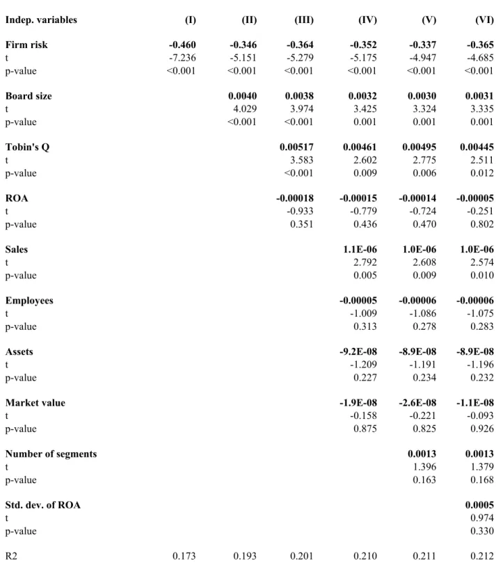
I will focus on Proposition 2. This is a truly new implication of my model that can be tested with the
data I have. It imposes a very strong restriction on observed behavior: the effect of risk on diversity should
have the opposite sign as the effect of diversity on incentive pay. In order to test this proposition, I regress
diversity on risk (and other controls) and incentive pay on diversityand risk (since I am concerned about
thepartial effects of diversity on incentive pay, keeping risk constant). I need both coefficients (diversity on risk and incentive pay on diversity) to be significantly different from zero and to have opposite signs. In order to appreciate the empirical strategy, suppose that onefinds (as I do) that diversity is
signif-icantly negatively related to firm risk. Thisfinding can be easily explained by the theory: homogeneity
and incentive pay are substitutes, therefore increasing risk makes the firm substitute incentive pay for
homogeneity. However, although the result is interesting by itself, it is still not a test of the theory.
The theory implies that, if homogeneity and incentive pay are substitutes, more diversity should increase
incentive pay, after controlling for the direct effects of risk on incentive pay. Therefore, if one finds zero or negative effects of diversity on incentive pay, the theory will be rejected.
3.4
Discussion
Here I discuss the intuition behind the results above. The symmetry property of Proposition 5 implies
that the concept of substitutability is well-defined; i.e. if incentive pay increases with the marginal cost
of homogeneity, work force homogeneity also increases with risk. But when can we expect to see incentive
pay and work force homogeneity being complements or substitutes? In what follows, I will focus on the
2 0
See Prendergast (1999) for a survey.
2 1
equilibrium relationship between work force homogeneity and incentive pay in (17), because they will be
complements if that derivative is positive and substitutes if it is negative.
Real world compensation contracts seem to offer weak explicit incentives to exert effort.22 It is controversial, however, whether standard moral hazard models imply that incentives should be
high-powered. Another view is that the basic moral hazard model that emphasizes the trade-offbetween risk and incentives is oversimplified and do not account for the main reasons why incentives might be weak.
Models along these lines can be found in Holmstrom and Milgrom (1991) and Baker (1992), among others.
The common feature of these models is that incentives linked to observable performance measures may
induce agents to take dysfunctional actions.23 In this section, I show that group loyalty may imply weak
incentives due to a related but different reason. Although in my model there is only one action that can be taken, this action has two different effects that agents care about: it affects the worker’s own pay and it affects her colleague’s pay.
The first thing to notice is that when group loyalty is at its minimum (in this case it may be more
accurate to call it group rivalry), incentives are muted:24
lim
α→−1a
∗ = 0 (22)
This happens because each agent is motivated by two different objectives: to increase her own pay and to decrease the other worker’s pay. While this might not be the most reasonable case (if firms have any
choice overα,they would never choose this level of group loyalty), it logically follows from the fact agents
have only one instrument (effort) to achieve two conflicting goals. The limiting case is the one in which these two opposing forces completely offset each other.
More interestingly, the power of incentives is also decreasing for high levels of group loyalty. Again,
when group loyalty unboundedly increases we have
lim
α→∞a
∗ = 0 (23)
When group loyalty is positive, the only instrument (effort) can be used to achieve two congruent goals. Therefore, theperceived power of incentives may be strong, even when the bonus rateais low. Therefore,
with more homogeneityα,the same level of effort can be achieved with a lowera,implying that there is
2 2 A well-known study that suggests that incentives are low-powered in executive compensation is Jensen and Murphy
(1990). See also Prendergast (1999) for a comprehensive review of the empirical literature on incentives infirms.
2 3
This interpretation is in Gibbons (1998).
2 4
a point in which more homogeneity will be used as a means of reducingain order to decrease the amount
of risk faced by the agents.25
Assuming a given uncertainty parameter c, the slope of equilibrium relationship between incentive
pay and work force homogeneity is given by (17). Simple algebra reveals that incentive payfirst increases
and then decreases with homogeneity. This implies that:
Proposition 6 Incentive pay increases with diversity when the marginal cost of homogeneity is low and decreases with diversity when the marginal cost of homogeneity is high.
We also have a related result:
Proposition 7 Incentive pay increases with diversity when risk is low and decreases with diversity when risk is high.
Propositions 6 and 7 do not tell us whether work force homogeneity and incentive pay are complements
or substitutes, but they give us a hint. Because profits monotonically decrease with both risk and the
marginal cost of homogeneity, market selection will drive mostfirms with high risk and high homogeneity
costs out of the market. In other words, firms in which incentive pay and work force homogeneity are
complements are always less profitable than firms in which incentive pay and work force homogeneity are
substitutes. Therefore, the substitution effect is the one most likely to be found, especially when observed diversity is low.
4
Learning
In this section I extend the previous model to allow workers to learn about each others’ types. I assume
that workers do not know each others’ characteristics, but repeated interactions among them lead to
gradual learning about each others’ types. Learning will affect group loyalty; therefore, to the extent that managers can organize work in ways that make interactions among workers more or less frequent,
managers will have some control over the loyalty level of their work force. This creates a link between
the organization of work and the provision of incentives in firms. The way work is organized depends
not only on technological or organizational constraints, but also on “human relations” constraints: how
different people are expected to react when interacting in the workplace.
2 5 This result may have interesting consequences. Luttmer (2001) argues that the relative low levels of redistribution
The main result in this section can be summarized as follows. From the principal’s standpoint,
allowing workers to meet very often in the workplace introduces risk, because learning can either increase
or decrease group loyalty. Therefore, whether the principal wants to promote or prevent interactions
among workers depends on her degree of risk-tolerance. I show that the profit function is convex for low
values of group loyalty and concave for high values of group loyalty. Therefore, the principal is more likely
to prevent interactions when workers are expected to be similar and more likely to promote interactions
when workers are expected to be different from each other. The intuition is that, when expected similarity is high, there is not much to gain if expectations are confirmed, but a lot to lose if they are not. With
the extra assumption that observable and unobservable similarity are positively correlated, the testable
implication is that the number of interactions (meetings) in the workplace should be positively related
to observed diversity.
4.1
Similarity
When allowing for uncertainty about workers’ types, many types of asymmetric information problems
may arise. For example, each worker may know her own type, but not her coworker’s type. The principal
may know more than some of the agents, or the agents may know each other’s type better than the
principal. To abstract from these problems and focus only on the learning problem, in this section I
assume that both agents and the principal have the same information at all stages of the game; i.e.,
αi =E[γ(vi, vj)|Ii] =E[γ(vi, vj)|Ij] =αj =α (24)
and that the principal always knows α.The assumption here is that knowledge of their own type does
not affect the expected value of similarity.26 Without this assumption, α
i may differ between workers,
which complicates the analyses without any expected extra implications.27
The timing of the game is modified as follows. In period0, the manager chooses two workers based
on their observed characteristics. Now, because there are some characteristics that are not observable,
one can think of the principal choosing a distribution of the random variable α, which may depend on
observed characteristics. In period1, before contracts are written, manager and workers jointly observe a
2 6 One possible situation in which that happens is one where types are uniformly distributed on a circle and similarity is
a function of distance between two types.
2 7 In Appendix C, I sketch an alternative model that allows for asymmetric information about similarity and show
common signalsof the true unknown variableγ. Then, they estimate the loyalty parameter based on the
observed signal and the prior distribution of γ. Then, everything is as before. In principle, there could
be many rounds of learning, as workers interact more and more over time. The manager can promote or
reduce interactions by the organization of work and task design, but she must do this before signals are
observed.
I assume that the prior distribution of γ is normal with meanγ0 and variance σ2
0. This means that,
in the ex ante stage, the principal chooses a pair ¡γ0,σ 2 0 ¢
.
4.2
Learning Technology
The learning technology is given by
st=γt+ut (25)
where ut is a zero-mean independent normal random variable with varianceσ2u.28
Equation (25) represents a standard signal-extraction problem. Both workers want to estimate the
true similarity between them γt given a collectively observed noisy signal st. Let the common prior
be given by γ0 and σ 2
0. Workers optimally update their beliefs. In this normal environment, Bayesian
updating is equivalent to least squares learning.
The least squares updating rule is given by
b
γt+1 = (1−βt)bγt+βtst (26)
σ2
t+1= (1−βt) 2
σ2 t+β
2 tσ
2
u (27)
βt= σ
2 t σ2
t +σ2u
(28)
It is assumed that perceived similarity will positively affect group loyalty. Of course, learning can only occur when workers interact. More socializing leads to lowerσ2
u. Whether this increases or decreases
group loyalty depends on the true similarity between workers relative to their prior beliefs.
2 8 One could also have a state-space representation of the learning technology by adding the following equation:
γt+1=ργt+εt+1
4.3
Interactions in the Workplace
Let us define the amount of interactions as the precision of the signalω =¡σ2 u
¢−1
. Assume now that the
firm can choose the amount of interactions ω between workers. For example, firms can put two workers
to work in the same room or in separate rooms, therefore affecting the likelihood that they interact. Also,
firms can assign two workers to different non-overlapping shifts or to the same shift.
For eachfirm, there is an optimal amount of interactions determined by technological and
organiza-tional parameters. For example, suppose a machine needs to be operated 24 hours a day, requiring the
supervision of only one worker at any time. Then, three workers working 8 non-overlapping hours a day
will be the efficient arrangement. But then workers will not interact. If the firm wants to increase the amount of interactions, it can pay one extra hour to each worker so their shifts will overlap an extra
hour each. Therefore, there is a cost in choosing a different amount of interactions than the one that is technologically efficient. The same can be said when firms want to reduce interactions. Suppose it is optimal to have workers in the same room because they can communicate faster. However, if firms want
to reduce the amount of interactions, they can put workers in separate rooms, but then communication
will be costlier.
Let ω0 be the optimal amount of interactions determined only by technological and organizational
conditions. Ifωis the level of interactions chosen by thefirm, interaction costs areC¡ωω0¢, withC(1) = 0,
C0 >0 ifω>ω0,C0 <0 ifω<ω0andC00>0.
4.4
Equilibrium
Suppose that the manager randomly selects two workers from a population with mean similarityγ0 and
variance σ2
0. Workers also have the common priors γ0 and σ 2
0 . In section 3, I derived a profit function
for the firm as a function of group loyalty, V∗(α) from equation (14). Now, profits also depend on the
similarity between the two types and on the level of interactions:
π¡ω1, ...,ωT;ω0,γ,γ0,σ2 0 ¢
=
T X
t=0
βtEhV∗¡bγt+1 ¢
−C³ωt
ω0
´i
(29)
The manager must choose an amount of interactions, which is a sequence(ω1, ...,ωT), that maximizes
(29) subject to (26), (27) and (28). Let us focus on the simplest case in whichT = 1.29 The maximization
problem can be written as max ω0 E " V∗ Ã
γ0+ σ
2 0 σ2 0+ 1 ω0
(s0−γ0) !
−C³ω0
ω0
´#
(30)
Assuming an interior solution,30 thefirst-order condition is
σ2 0 ¡
σ2 0ω0+ 1
¢2E £
(s0−γ0)V∗0(bγ1) ¤
= 1
ω0C 0³ω0
ω0
´
(31)
Whether the manager wants to facilitate (ω0 >ω0) or hinder interactions (ω0 <ω0) depends on the
sign of E[(s0−γ0)V∗0(1−bγ1)]. It is easy to show that
cov£s0−γ0, V∗0(bγ1) ¤
≷0 ifV∗00≷0 (32)
From manager’s viewpoint,
E(s0−γ0) =γ0−γ0 = 0 (33)
Therefore, the following proposition is straightforward:
Proposition 8 The manager wants to promote interactions if V∗ is convex and to avoid interactions if
V∗ is concave.
The intuition is that the principal would like to promote interactions whenever learning is likely to
increase perceived similarity between the two workers. But the learning process is unbiased ex ante,
therefore from the manager’s viewpoint it only introduces uncertainty. Thus, the manager is more likely
to profit from learning the more risk-tolerant she is. This is why the concavity of functionV∗ matters.
The question now is to know whenV∗ is going to be concave or convex. Manipulation ofV∗ leads to
the following proposition:
Proposition 9 There exists λ≥0 such that V∗ is convex whenever α∈(−1−λ,−1 +λ) and concave otherwise.
Therefore, this proposition says thatV∗ is concave whenever work force homogeneity is expected to
be very high or very low, while it is convex for low absolute values of α.31
3 0 A sufficient condition for the solution to be interior islim
x→∞C(x) = limx→0C(x) =∞.
3 1 How can we understand this result? Noticefirst that functionV∗(α)is bounded below by zero and above byVF B
,the first-best level of profits. As we have seen before, profits are increasing inαforα>−1,thereforeV∗(α)has to eventually become concave forαsufficiently large. For values ofαless than−1,the opposite occurs: V∗(α)is decreasing inα.This is because group rivalry is so strong thatfirms can actually profit from it in a rather bizarre way: the piece-rateais negative, which makes worker i exert effort because of her desire to harm worker j. (For evidence that individuals are sometimes willing to incur in losses in order to punish other people, see for example Fehr, Gachter and Kirchsteiger (1997)). When
I have assumed an unbounded support for α so I could work with normal distributions. However,
while logically plausible, compensation contracts with negative piece-rates (the case implied by α<−1)
are not observed in the real world. For the interpretation of the results, I will then focus on the empirically
relevant case of α>−1.
If thefirm expects workers to be very similar, i.e.,γ0 is very high, profits are close to thefirst-best
level. Therefore, there is not much to gain on the upside, but a lot to lose on the downside: if workers
learn that they are not as similar as they once thought they were, profits can fall dramatically. Therefore,
the more similar workers are expected to be, the less likely firms are to promote interactions between
them in the workplace. On the other hand, for values ofγ0 close to−1,firms can gain a lot on the upside
and do not lose much on the downside, therefore they would be more willing to promote learning.
Finally, letη be a (scalar) measure of similarity between two workersbased only on their observable
characteristics. I make the following assumption:
Assumption A3 E[γ|η]is non-decreasing in η.
This assumption just says that people who are similar in observable characteristics expect themselves
to be similar after they learn about unobservable characteristics as well. Notice that this assumption
will hold unless similarity in observable characteristics is very negatively correlated with similarity in
unobservable characteristics.
The following assumption is similar to A2:
Assumption A4 E[γ|η]>−1.
With the assumptions above and Propositions 8 and 9, we finally have:
Proposition 10 If A3 and A4 hold, the principal will choose to prevent interactions when workers are expected to be similar. When they are expected to be different, she will choose to promote interactions.
In what follows, I test this implication by regressing a measure of interactions in the workplace on
observed diversity. If the model is true, interactions should be positively related to diversity.
4.5
When Social Interactions Increase Group Loyalty
among them. I have ignored the direct effect of interactions on cooperation, so here I consider the case in which more meetings imply more cooperation. To simplify the argument, I now ignore any learning
considerations.
The result here is almost trivial:
Proposition 11 If more interactions in the workplace increase cooperation, then the principal always wants to promote interactions.
The proof is immediate given that C0(1) = 0, that is, a small increase in the frequency of meetings
has negligible costs, but it has a positive effect on profits. However, it can also be shown that the effect of diversity on meetings in this case can be either positive or negative. Therefore, if we assume that
both forces (learning and socializing) are operating, one would still expect a positive correlation between
diversity and interactions.
5
Data
In the next section, I provide new evidence that is compatible with the main implications of the model. I
focus on three empirical relationships: diversity andfirm risk, diversity and incentives, and diversity and
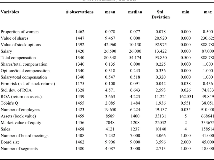
interactions in the workplace. The relevant unit of study will be the board of directors of 1462 publicly
tradedfirms infiscal year 1998.
In what follows, it is important to understand the role of the model in the design of the empirical
strategy. As we have seen above, the model predicts certain correlations between diversity and other
variables. I look for these correlations in the data. In order to do that, I have to find empirical proxies
for the theoretical variables. Some of these proxies capture the spirit of their theoretical counterparts,
but they may not be exact analogs of the variables in the model. For example, in the model I work with
the concept of pairwise diversity (or similarity) for simplicity. When I get to the data, teams (boards of
directors) have many members, so I have to empirically define diversity at the team level instead of using
pairwise measures. Also, reality is too complex, so many other issues that are ignored in the model may
be present in the data. Therefore, I use many variables that were not explicitly taken into consideration in
the theoretical part of this paper. Finally, the model is too simplified to be useful in structural estimation,
therefore I only look for correlations between relevant variables using empirically-motivated functional
5.1
Why Use Corporate Boards?
Corporate boards are good empirical examples of teams because the individual output of each director
cannot be directly measured. Compensation is linked to firm performance mainly through grants of
restricted shares and options. Director compensation has a simple structure. Directors are paid a fixed
annual salary, plus fees for attending meetings and shares and stock options. Therefore, if directors have
any effect on the market value of their firms, this compensation scheme suffers from the 1/n problem (free-riding).
The theory assumes that firms can choose both compensation contracts and the composition of the
work force as means of providing incentives to agents.32 Therefore, directors must be subjected to
performance-based compensation contracts in order for the theory to be valid. A substantial fraction of
non-employee directors’ compensation is composed of restricted shares and stock options (about 45% of
total compensation, on average. See Table 1).33 About 80% of the firms in my sample granted shares
and/or options to their directors. Shares and options almost always come with restrictions. Although
restrictions vary acrossfirms, usually directors are granted restricted stock which they then get once they
leave the firm. Options usually come with vesting requirements and they may or may not be exercisable
if the director leaves the firm.34 Assuming that directors cannot completely hedge firm-specific risks
that come with restricted shares and options (or that it is too costly to do so), an increase in the grant
of shares and/or options will increase their alignment with shareholders’ objectives, provided everything
else is constant.35
Because information on directors is usually available to the public (due to regulations, listing
require-3 2 Other papers have also looked at the determinants of board composition. For example, Hermalin and Weisbach (1988)
have found that inside directors are more likely to be replaced by outside directors after poorfirm performance. Klein (1998) finds thatfirms with more complex financing have more investment bankers, pharmaceuticalfirms have more academics, defense industry firms have more ex-politicians and ex-military on the board. Aggarwal and Knoeber (2001) relate the number of political directors on the board to variables characterizing thefirm’s need for political directors. As in this paper, they allfind evidence consistent withfirms optimally choosing directors for their characteristics. However, this paper is the first to study the homogeneity of the board as an endogenously determined variable.
3 3
Here I only consider non-employee directors. Employee directors are usually not specifically paid for their duties as directors and have individually designed compensation contracts.
3 4
As an example, the American Home Products Corporation’s proxy statement says “the options become exercisable at the date of the next annual meeting or earlier in the event of the directors termination of service, provided that the optionee has completed at least 2 years of service as a director at the time of exercise or termination”.
3 5 If directors could always hedge firm-specific risks, no incentive contract could ever be binding. Both theoretical and
ments or shareholder activism), measures of diversity can be constructed using demographic information
on individual directors. In this paper I use the proportion of women on boards as a measure of diversity.
I also briefly discuss the distinction between inside and outside directors as a measure of diversity. The
analysis in this paper could also be extended to include other variables such as ethnicity, tenure in the
firm, educational background, and so on, provided one is willing to collect these data.36
Another good reason for using data on boards is that we know how many meetings they have every
year. Therefore, we have an intuitive measure of interactions in the workplace, which is the number of
board meetings. A board meeting is an important input in the production of advising and monitoring
(Adams, 2001), but it is also costly because directors are usually paid for attending meetings. This fits
well with the theoretical assumption that interactions have both benefits and costs that are unrelated to
the composition of the work force.
Also important is the fact that boards perform roughly the same functions in different firms, which makes cross-sectional comparisons of boards more palatable than of most other kinds of work teams.
One possible problem with using corporate boards, however, is that although directors are
sharehold-ers’ agents, the shareholders themselves are not acting as the principal in the theory, i.e. they are not the
ones writing incentive contracts. Therefore, the assumption here is that compensation contracts, hiring
decisions and organizational choices are such that they maximize shareholder value, even if we could not
directly observe an active principal making all these choices. The tests that follow can be seen as joint
tests of the effects of diversity on behavior and of value-maximizing corporate behavior.37
5.2
Data Description
The choice of the sample was driven mainly by data availability. I started with the data set collected
by Adams (2001) and Adams, Almeida and Ferreira (2001).38 It contains detailed firm-, board- and
director-level data from 358 Fortune 500firms (excluding utilities andfinancialfirms) infiscal year 1998.
Data from previous years were also used to construct measures of volatility. Sources are proxy statements,
Compustat, CRSP, ExecuComp, Moody’s Manuals and firms’ web sites.
This initial sample was then expanded in two ways. First, by collecting director compensation variables
for the original firms. Second, by increasing the sample size in the following manner. I selected allfirms
3 6 I intend to collect data on where directors went to school, the states they came from, and so on.
3 7 For a survey of the economic literature on boards of directors, see Hermalin and Weisbach (2001).
in the ExecuComp database for which at least some data on directors’ compensation were available.39
Then, I looked for the names of their directors in the 1999 “Directory of Corporate Affiliations”.40 The final sample has 1462 firms.
To construct the variable measuring the sex composition of boards, I had to infer gender from directors’
first names. In the original sample that was done directly from proxy statements. For the remaining
observations in thefinal sample, I relied on the information in the “Directory of Corporate Affiliations”. In order to minimize errors, I used many name dictionaries, including some language-specific ones (English,
Hebrew and Arabic). Still, some ambiguities remained, especially in some few cases in whichfirst names
were abbreviated.
I constructed a simple measure of diversity, which is the fraction of female directors on boards.41
As one can see from Table 1, the proportion of women on boards ranges from zero to 50%. Therefore,
the proportion of women is a monotonic measure of diversity: higher fractions of women imply more
diversity. Few women sit on boards. On average, only about 8% of directors are women (see Table 1).
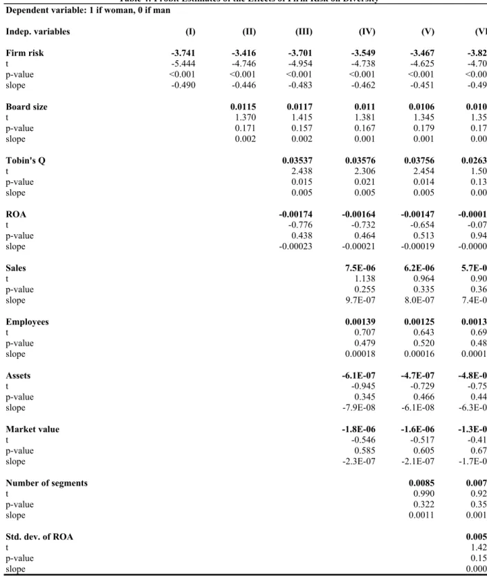
In order to test the relationship between diversity and risk, I need a measure of firm risk that
af-fects directors’ compensation. Following Aggarwal and Samwick (1999), I use the standard deviation of
monthly stock returns to proxy for σ in Holmstrom and Milgrom’s linear contracts model. Since
incen-tives to directors are mainly provided by stock ownership, this measure seems reasonable. This standard
deviation was computed using monthly stock returns from 1993 to 1998.42
Incentive pay to directors is provided by grants of shares and stock options. Shares and options are
usually granted at annual meetings. In order to be precise and to avoid having to adjust for stock splits,
I collected data of market prices of shares at the end of the month of each firm’s annual meeting for
the 1998 fiscal year. It is unfeasible to correctly price restricted shares and options. Restricted shares
should not have the same value as ordinary shares and restrictions vary too much acrossfirms to justify
any simple adjustment procedure. Options are even more complicated because, on top of their vesting
requirements, they can only be priced using some option-pricing theory. As in virtually all compensation
papers (see Jensen and Murphy, 1990, and Aggarwal and Samwick, 1999), I ignore restrictions and vesting
3 9
This expanded sample is also being used by Adams and Ferreira (work in progress). I thank Renée Adams for spending a great part of her time in actual collecting and helping me collect these data.
4 0
Directory of Corporate Affiliations, Volume 3, U.S. Public Companies, 1999, published by National Register Publishing.
4 1
When a given director’s gender could not be inferred by his/her name, I attributed the sample mean proportion of women to that director, instead of 1 (woman) or 0 (man).
4 2