Construction of Tightened-Normal- Tightened Schemes of Type TNT-(n1, n2; c) Indexed through Nano Quality Levels

Construction of

Tightened-Normal-Tightened Schemes of Type TNT-(n

1

, n

2

; c)

Indexed through Nano Quality Levels

R. RADHAKRISHNAN

Associate Professor in Statistics, PSG College of Arts & Science,

Coimbatore, Tamilnadu, India. Email: [email protected]

P. VINOTHA

Research Scholar PSG College of Arts & Science,

Coimbatore, Tamilnadu, India. Email: [email protected]

Abstract

Motorola (1980) introduced the concept of six sigma as a quality philosophy and a management strategy, which when adopted in a system of organization will reduce wastages and increase the profit to the management results in enhancing the satisfaction of the customer. If this concept of Six Sigma is adopted in an organization it can results in 3.4 or lower number of defects per million opportunities in the long run. In recent days many companies in developed and developing countries started working beyond Six Sigma level and thereby the performance level increases with number of defectives reduced to near zero level. In those situations a more stringent quality level than six sigma quality level is regarded to construct the sampling plan. In this paper a procedure for the construction of Tightened-Normal-Tightened Schemes of Type TNT-(n1, n2; c)

indexed through producer’s Nano quality level (PNQL) and consumer’s Nano quality level (CNQL) is presented and suitable tables are also provided for the easy selection of the plans.

Keywords: Nano Quality Level, Poisson distribution, Tightened-Normal-Tightened Schemes, Operating Characteristic curve, Six sigma Quality Level (SSQL).

Introduction

A single defective unit of the sample, in a compliance testing, calls for rejection of the entire lot. To overcome this undesirability, Tightened-Normal-Tightened (TNT) sampling scheme was developed by Calvin (1977). This scheme utilizes two single sampling plans (with c=0) of different sample sizes together with switching rules to create swelling in the upper portion of the OC curve. Soundararajan and Vijayaraghavan (1992) studied the TNT scheme by assuming ‘c’ to take values of other than zero, the scheme can be designated as TNT-(n1, n2; c) which refers to a TNT scheme where the normal and tightened single sampling plans have the

acceptance number c, but on tightened inspection the sample size is n1 and on normal inspection the sample size

is n2 (< n1).

Producer’s Nano Quality Level and Consumer’s Nano Quality Level

The proportion defective corresponding to the probability of acceptance 1-γ1, γ1=10-9 in the OC

(Operating Characteristic) curve is termed as Producer’s Nano Quality Level (PNQL). The new sampling plan is constructed with a point on the OC curve (PNQL, 1-γ1), similar to (AQL, 1-α), α=0.05 suggested by Dodge and

Roming (1942) and (SSQL-1, 1-α1), α1=3.4x10-6 suggested by Radhakrishnan and Sivakumaran (2008).

Similarly a new Sampling plan can be constructed with a point on the OC curve (CNQL, γ2), γ2=2γ1 is similar to

(LQL, β), β=2α suggested by Dodge and Roming (1942) and (SSQL-2, β1), β1=2α1 suggested by

Radhakrishnan and Sivakumaran (2008).

Conditions for Application

• Production is continuous, so that results of the past, present and future lots are broadly the indicative of a continuous process.

• Lots are submitted sequentially.

• Inspection is by attributes, with the lot quality level defined as the proportion defective.

• Human involvement is to be minimum in the manufacturing process.

• The companies are to have sufficient knowledge and experience in adopting Six Sigma initiatives in their process to ensure the system has the potentiality to produce nearly zero defectives.

Operating procedure

Step 1: Inspect under tightened inspection, using the single sampling plan with sample size n1 and acceptance number c. If‘t’ lots in a row are accepted, switch to normal

inspection (Step 2).

Step 2: Inspect under normal inspection, using the single sampling plan with sample size n2 (< n1) and acceptance number c. Switch to tightened inspection, after a

rejection, if an additional lot is rejected in the next‘s’ lots.

Thus, the TNT-(n1, n2; c) sampling scheme is specified by the parameters n1, n2, c, s and t, constitute the

criteria for switching to tightened and normal inspection respectively.

Operating Characteristic function

Under Poisson Model the OC function of the TNT scheme given by Calvin (1977) is,

Under the conditions for application of Poisson model for the OC curve, P1 and P2 are defined as

The OC function of TNT scheme corresponds to the scheme OC function of MIL-STD-105D for S=4 and t=5 [Hald and Thyregod (1965); Dodge (1965); Calvin (1977)].

Construction of TNT-(n1, n2; c) Schemes Indexed through PNQL

By fixing the probability of acceptance of the lot, Pa (p) as 1-10-9with Poisson distribution as the basic

distribution and from equation (1), the values of nPNQL are obtained for various combinations of ‘c’ and ‘k’ using Excel package and presented in Table-1. The sample size ‘n = n2’ of the normal plan is obtained as n2 =

nPNQL/PNQL and then the sample size n1 of the tightened plan is found as n1= kn2 (k>1). Hence the

parameters of the TNT-(n1, n2; c) schemes n1, n2 and c are obtained for various values of PNQL.

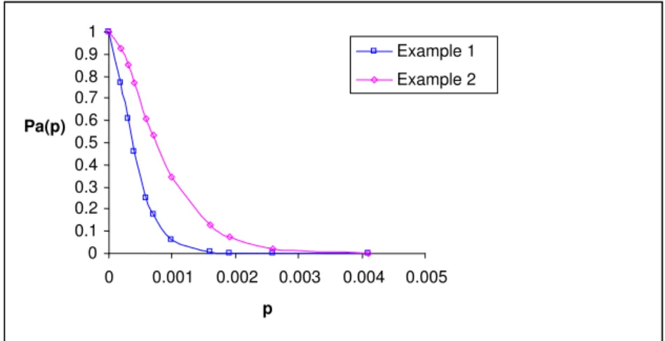
Example 1:

For a given PNQL = 0.00000002, c=1 and k=2.0 the value of nPNQL is selected from Table-1 as 0.0000450 and the corresponding sample size of normal plan ‘n2’ is computed as n2

=0.0000450/0.00000002=2250 and the sample size of tightened plan n1 is computed as n1=(2.0)(2250)=4500.

Hence the parameters of TNT-(n1, n2; c) are n1 =4500, n2 =2250 and c=1 for a specified PNQL = 0.00000002.

Practical Application

In a bolt manufacturing company, if the manufacturer of bolts fixes the quality of bolt as PNQL=0.00000002 (2 non-confirming bolt out of 10 crore items), then inspect under tightened inspection with sample of size 4500 bolts and acceptance number c=1 from the manufactured lot of a particular month. If 5 lots in a row are accepted under tightened inspection, then switch to normal inspection, then inspect under normal inspection with a sample of 2250 bolts and acceptance number c=1 from the manufactured lot of a particular month. Switch to tightened inspection, after a rejection, if an additional lot is rejected in the next 4 lots and inform the management for corrective action.

Example 2:

For a given PNQL = 0.0000007, c=2 and k=2.25 the value of nPNQL is selected from Table-1 as 0.0018470 and the corresponding sample size of normal plan ‘n2’is computed as n2 = 0.0018470 /0.0000007 =

2639 and the sample size of tightened plan n1 is computed as n1 = (2.25)(2639) =5938. Hence the parameters

of TNT-(n1, n2; c) are n1 =5938, n2 =2639 and c=2 for a specified PNQL = 0.0000007.

The OC curves of the schemes provided in Example 1 and Example 2 are presented in Figure1.

Figure 1: OC curves for the schemes n1 = 4500, n2 = 2250, c=1 & n1 = 5938, n2 = 2639, c=2

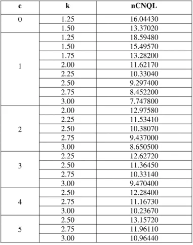
Construction of TNT-(n1, n2; c) Schemes Indexed through CNQL

By fixing the probability of acceptance of the lot as γ2=2γ1, where

γ

−

= with Poisson distribution as the basic distribution and from equation (1), the values of nCNQL are obtained for various combinations of ‘c’ and ‘k’ using Excel package and presented in Table-2. The sample size ‘n = n2’ of the

normal plan is obtained as n2 = nCNQL/CNQL and then the sample size ‘n1’ of the tightened plan is found as

n1= kn2 (k>1). Hence the parameters of the TNT-(n1, n2; c) schemes n1, n2 and c are obtained for various

values of CNQL.

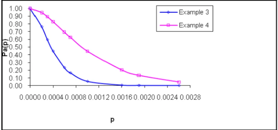
Example 3:

For a given CNQL = 0.005, c=1 and k=2.50 the value of nCNQL is selected from Table-2 as 9.2974 and the corresponding sample size of normal plan ‘n2’is computed as n2 = 9.2974/0.005=1859 and the sample

size of tightened plan n1 is computed as n1=(2.50)(1859)=4648. Hence the parameters of TNT-(n1, n2; c) are n1

=4648, n2 =1859 and c=1 for a specified CNQL = 0.005.

Practical Application

In a bolt distributing company, if the distributor of bolts fixes the quality of bolt as CNQL=0.005 (5 non-confirming cell bolts out of 1000 items), then inspect under tightened inspection with sample of size 4648 bolts and acceptance number c=1 from the distributor lot of a particular day/week. If 5 lots in a row are accepted under tightened inspection, then switch to normal inspection, then inspect under normal inspection with a sample of 1859 bolts and acceptance number c=1 from the distributor lot of a particular day/week. Switch to tightened inspection, after a rejection, if an additional lot is rejected in the next 4 lots and inform the management for corrective action.

0 0.1 0.2 0.3 0.4 0.5 0.6 0.7 0.8 0.9 1

0 0.001 0.002 0.003 0.004 0.005

p Pa(p)

Example 1

Example 4:

For a given CNQL = 0.006, c=2 and k=2.25 the value of nPNQL is selected from Table-2 as 11.53410 and the corresponding sample size of normal plan ‘n2’is computed as n2 = 11.53410/0.006=1922

and the sample size of tightened plan n1 is computed as n1=(2.25)(1922)=4325. Hence the parameters of

TNT-(n1, n2; c) are n1 =4325, n2 =1922 and c=2for a specified CNQL = 0.006.

The OC curves of the schemes provided in Example 3 and Example 4 are presented in Figure 2.

Figure 2: OC curves for the schemes n1 = 4648, n2 = 1859, c=1 & n1 = 1922, n2 = 4325, c=2

Table 1: Parameters of TNT-(n1, n2; c) schemes for a specified PNQL

c k nPNQL

0 1.25 0.00000000105 1.50 0.00000000105

1

1.25 0.0000450 1.50 0.0000450 1.75 0.0000450 2.00 0.0000450 2.25 0.0000450 2.50 0.0000450 2.75 0.0000450 3.00 0.0000450

2

2.00 0.0018470 2.25 0.0018470 2.50 0.0018470 2.75 0.0018470 3.00 0.0018470 3

2.25 0.0126300 2.50 0.0126300 2.75 0.0126300 3.00 0.0126300 4

2.50 0.0419860 2.75 0.0419860 3.00 0.0419860 5

Table 2: Parameters of TNT-(n1, n2; c) schemes for a specified CNQL

c k nCNQL

0 1.25 16.04430 1.50 13.37020

1

1.25 18.59480 1.50 15.49570 1.75 13.28200 2.00 11.62170 2.25 10.33040 2.50 9.297400 2.75 8.452200 3.00 7.747800

2

2.00 12.97580 2.25 11.53410 2.50 10.38070 2.75 9.437000 3.00 8.650500 3

2.25 12.62720 2.50 11.36450 2.75 10.33140 3.00 9.470400 4

2.50 12.28400 2.75 11.16730 3.00 10.23670 5

2.50 13.15720 2.75 11.96110 3.00 10.96440

Conclusion

In this paper a new concept Nano Quality with two quality levels such as Producer’s Nano Quality Level (PNQL) and Consumer’s Nano Quality Level (CNQL) is introduced and the procedure for constructing Tightened-Normal-Tightened Schemes of Type TNT-(n1, n2; c) indexed through these quality levels with

Poisson distribution as the base line distribution are also presented. The procedure indicated in this paper can replace the existing quality levels adopted in the construction of sampling plans because more organizations have specialized in adopting Six Sigma in their system and are willing to shift towards Nano Technology that will results in nearly zero non-conformities. So it is necessary for those companies to adopt the quality levels in the construction of the plan suggested in this paper. This will increase the confidence of the producer in providing a better sampling inspection procedure in enhancing the satisfaction of the consumers. The procedure outlined in this paper can be used for other plans also.

References

[1] T.W. Calvin, TNT zero acceptance number sampling, American Society for Quality Annual Technical Conference Transactions, Philadelphia, PA, 1977, pp.35-39.

[2] H.F. Dodge, Notes on the evaluation of Acceptance Sampling Plans, Part I, Journal of Quality Technology, 1969, Vol.1, No.2, pp.77-78.

[3] H.F. Dodge and H.G. Roming, Army service forces tables, Bell telephone laboratories, United States, 1942.

[4] Norio Taniguchi, On the basic concept of Nano-Technology, Proc. Intl. Conf. Prod. Eng. Tokyo, Part II, Japan Society of Precision Engineering, 1974.

[5] R. Radhakrishnan, Contributions to the study on selection of certain Acceptance Sampling Plans, Ph.D thesis, Bharathiar University, Coimbatore, India, 2002.

[6] R. Radhakrishnan, Construction of Six Sigma based Sampling Plans, Post Doctoral Thesis (D.Sc), submitted to Bharathiar University, Tamilnadu, India, 2009.

[7] R. Radhakrishnan, and P.K. Sivakumaran, Construction and Selection of Six Sigma Sampling Plan indexed through Six Sigma Quality Level, International Journal of Statistics and Systems, 2008, Vol.3, No.2, pp.153-159.

[8] R. Radhakrishnan, and P. Vinotha, Construction of Sampling plans indexed through Producer’s and Consumer’s Nano Quality Levels, International Journal of Nano Technology and Applications , 2011a, Vol 5, N0.1, pp.1-7.

[9] R. Radhakrishnan, and P. Vinotha, Construction of Repetitive Group Sampling plan Indexed through Producer’s Nano Quality Level and Consumer’s Nano Quality Level, International Journal of Recent Scientific Research , 2011b, Vol.2, Issue.2, pp.62-66.