Technical Note: A novel parameterization of the transmissivity due to ozone absorption in the <i>k</i>-distribution method and correlated-<i>k</i> approximation of Kato et al. (1999) over the UV band

www.atmos-chem-phys.net/15/7449/2015/ doi:10.5194/acp-15-7449-2015

© Author(s) 2015. CC Attribution 3.0 License.

Technical Note: A novel parameterization of the transmissivity due

to ozone absorption in the k-distribution method and correlated-k

approximation of Kato et al. (1999) over the UV band

W. Wandji Nyamsi1, A. Arola2, P. Blanc1, A. V. Lindfors2, V. Cesnulyte2,3, M. R. A. Pitkänen2,3, and L. Wald1 1_{MINES ParisTech, PSL Research University, O.I.E., Centre Observation, Impacts, Energy, Sophia Antipolis, France} 2_{Finnish Meteorological Institute, Kuopio, Finland}

3_{Department of Applied Physics, University of Eastern Finland, Kuopio, Finland}

Correspondence to: W. Wandji Nyamsi (william.wandji@mines-paristech.fr)

Received: 21 October 2014 – Published in Atmos. Chem. Phys. Discuss.: 13 January 2015 Revised: 21 June 2015 – Accepted: 23 June 2015 – Published: 09 July 2015

Abstract. Thek-distribution method and the correlated-k ap-proximation of Kato et al. (1999) is a computationally ef-ficient approach originally designed for calculations of the broadband solar radiation at ground level by dividing the solar spectrum in 32 specific spectral bands from 240 to 4606 nm. Compared to a spectrally resolved computation, its performance in the UV band appears to be inaccurate, espe-cially in the spectral intervals #3 [283, 307] nm and #4 [307, 328] nm because of inaccuracy in modeling the transmissiv-ity due to ozone absorption. Numerical simulations presented in this paper indicate that a single effective ozone cross sec-tion is insufficient to accurately represent the transmissivity over each spectral interval. A novel parameterization of the transmissivity using more quadrature points yields maximum errors of respectively 0.0006 and 0.0143 for intervals #3 and #4. How to practically implement this new parameterization in a radiative transfer model is discussed for the case of li-bRadtran (library for radiative transfer). The new parameter-ization considerably improves the accuracy of the retrieval of irradiances in UV bands.

1 Introduction

Radiative transfer models (RTMs) are often used to provide estimates of the UV irradiance. One of the difficulties in the computation lies in taking into account the gaseous ab-sorption cross sections that are highly wavelength dependent (Molina and Molina, 1986). For instance, the ozone cross

section changes by more than 2 orders of magnitude over the UV band [280, 400] nm. The best estimate of the UV ir-radiance is made by a spectrally resolved calculation of the radiative transfer for each wavelength followed by integra-tion over the UV band. However, such spectrally detailed cal-culations are computationally expensive. Therefore, several methods have been proposed to reduce the number of calcu-lations. Among them are thek-distribution method and the correlated-k approximation proposed by Kato et al. (1999). It is originally designed for providing a good estimate of the total surface solar irradiance by using 32 specific spectral in-tervals across the solar spectrum from 240 to 4606 nm. Here-after, these spectral intervals are abbreviated as KBs (Kato bands). The Kato et al. method is implemented in several RTMs and is a very efficient way to speed up computations of the total surface solar irradiance. Its performance over the UV band is not very accurate when compared to detailed spectral calculations made with libRadtran (library for radia-tive transfer; Mayer et al., 2005) or SMARTS (Simple Model of the Atmospheric Radiative Transfer of Sunshine; Guey-mard, 1995).

For a spectral interval1λwhereλis the wavelength, let I01λ andI1λ denote respectively the irradiance on a

hori-zontal plane at the top of atmosphere and at the surface; the spectral clearness index KT1λ, also known as spectral global

transmissivity of the atmosphere, spectral atmospheric trans-mittance, or spectral atmospheric transmission, is defined as

KT1λ=

I1λ

I01λ

mospheric and cloud coverage states and for each KB. They found that the Kato et al. method underestimates transmis-sivity in KBs #3 [283, 307] nm and #4 [307, 328] nm – cov-ering the UV range by respectively−93 and−16 % in rel-ative value – and exhibits relrel-ative root mean square errors (RMSEs) of 123 and 17 % in clear-sky conditions. Similar relative errors are observed for cloudy conditions.

The underestimation for these two bands can be explained by the fact that Kato et al. (1999) assume that the ozone cross section at the center wavelength in each interval repre-sents the absorption over the whole interval. The ozone cross sections were taken from WMO (1985). Actually, the ozone cross section is strongly dependent on the wavelength in the UV region (Molina and Molina, 1986). Both KBs #3 and #4 in the UV range are large for considering only a single value of the ozone cross section.

In order to improve the potential of the Kato et al. method for estimating narrowband UV irradiances, in particular for the KBs #3 and #4, a new parameterization is proposed for the transmissivity due to the sole ozone absorption. Then, for each spectral interval, an assessment of the performance of the new parameterization in representing this transmissivity is made for a wide range of realistic cases against detailed spectral calculations. A short section describes how to imple-ment this parameterization in the practical case of the RTM libRadtran 1.7. Finally, in each KB, the performance of the new parameterization is assessed when the direct normal, up-ward, downup-ward, and global irradiances at different altitudes are computed.

2 Transmissivity due to ozone absorption

The average transmissivityTo31λ due to the sole ozone

ab-sorption for1λcan be defined by Eq. (2).

To31λ=

R

1λ

I0λe

−kλµu_0dλ R

1λ

I0λdλ

, (2)

whereIoλ is the spectral irradiance at the top of the

atmo-sphere on a horizontal plane,kλthe ozone cross section atλ,

uthe amount of ozone in the atmospheric column andµ0the cosine of the solar zenith angle.

A technique widely used for computingTo31λis based on

a discrete sum of selected exponential functions (Wiscombe and Evans, 1977):

wherekiare the effective ozone cross sections andai are the

weighting coefficients obeying

n

P

i=1 ai=1.

In the Kato et al. method, only one exponential function (n=1) is used for each KB to estimate the average transmis-sivityTo3KB:

To3KB=e

−kKB_µu

0_{. (4)}

Kato et al. (1999) have chosen the ozone cross section at the central wavelength for KB #3 and KB #4 for a temperature of 203 K:kKB3=5.84965×10−19cm2andkKB4=4.32825× 10−20_cm2_.

3 Effective ozone cross section

Is there a single effective ozone cross section that may rep-resent the absorption over the whole interval? If so, this ef-fective cross sectionkeffis determined for each KB from the combination of Eqs. (2) and (3) withn=1:

To3eff=e

−keff_µu 0 = 1

I01λ

Z

1λ

I0λe

−kλ_µu

0_{dλ. (5)}

This equation may be rewritten

keff u µ0

= −ln 1 I01λ

Z

1λ

I0λe

−kλµu_{0dλ. (6)}

Several simulations are made to study this hypothesis. The ozone cross sections are those from Molina and Molina (1986) at 226, 263 and 298 K, and the top-of-atmosphere so-lar spectrum of Gueymard (2004) is used. The ozone cross sections at 203 K are obtained by linear extrapolation for each wavelength (Fig. 1). Samples of 10 000 pairs(µ0, u) were generated by a Monte Carlo technique. The random se-lection of the solar zenith angles follows a uniform distribu-tion in [0◦_{, 80}◦_{]. Similarly to what was done by Lefèvre et}

al. (2013) and Oumbe et al. (2014),uis computed in Dobson units as

u=300β+100, (7)

whereβfollows the beta distribution with A parameter=2, and B parameter=2.

The 10 000 simulations yield a set X of (_µu

0)and a set Y of values−ln_I1

01λ R

1λ

I0λe

−kλµu_{0dλ; Eq. (6) is then}

Figure 1. Ozone cross sections at 203 K as a function of the wave-length.

andkeff can be found by least-square fitting technique. For KBs #3 and #4, the values obtained are respectivelykeff3= 2.29×10−19_cm2_andk

eff4=2.65×10−20cm2. The average transmissivityTo3eff with the effective ozone cross section is then computed with Eq. (5).

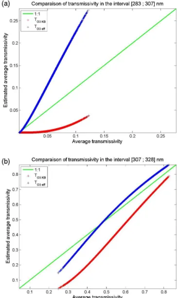
Estimated transmissivitiesTo3KB andTo3effcomputed with Eq. (4) and Eq. (5) using a second set of 10 000 pairs(µ0, u) randomly selected are compared to the reference transmis-sivity To31λ computed with Eq. (2) for each KB (Fig. 2).

In KB #3, To3KB (red line) strongly underestimates To31λ, meaning that the single ozone cross section adopted by Kato et al. is too large. On the contrary,To3eff(blue line) exhibits a large overestimation, meaning that the efficient ozone cross section keff is too low. That may be explained by the fact that the solar radiation at the short wavelengths is completely absorbed and therefore becomes somewhat unimportant for the effective ozone cross sections. In this interval, the ozone cross section is strongly variable as shown in Fig. 1. Since keff is the optimal value reducing as much as possible the discrepancy betweenTo3eff andTo31λ, it may be concluded that a single effective ozone cross section may not accurately represent the absorption over the whole KB #3.

In KB #4, To3KB (red line) noticeably underestimates To31λ, meaning that the single ozone cross section adopted

by Kato et al. is too large. To3eff is closer toTo31λ though it exhibits underestimation when To31λ<0.47 and

overesti-mation whenTo31λ>0.47. Like previously stated, it may be

concluded that a single effective ozone cross section may not accurately represent the absorption over the whole KB #4.

Figure 2. Scatterplot between average transmissivityT_o31λand the estimatedTo3KB(red line) andTo3eff(blue line) for (a) KB #3 [283, 307] nm and (b) KB #4 [307, 328] nm. The identity line is in green.

4 New parameterization

The new parameterizationTo3new for computingTo31λ con-sists in using Eq. (3) withn greater than 1 but as small as possible to decrease the number of calculations while retain-ing a sufficient accuracy.n can be seen as the number of sub-intervalsδλi included in1λfor which effective ozone

cross section and weighting coefficients can be defined. The greater then, the greater the number of calculations, the more accurate the modeling ofTo31λ.

Many solutions are possible. No systematic scan of possi-ble solutions inn, weightai andδλi was made. This could

Figure 3. Scatterplot between average transmissivityT_o31λand the estimatedTo3KB(red line) andTo3new(blue line) for (a) KB #3 [283, 307] nm and (b) KB #4 [307, 328] nm. The identity line is in green.

few tests were made with nranging from 2 to 5. The best trade-off was found atn=4. A further study was performed forn=4 by adopting equal weights for the sub-intervals for both KBs #3 and #4:

To3new= 4 X

i=1

0.25e−kiu/µ0_{, (9)}

whereki is the effective ozone cross section for each of the

four sub-intervals. This proposed solution is of empirical nature. Using a third set of 10 000 randomly selected pairs (µ0, u), from whichTo31λ is computed (Eq. 2), the optimal

sets of fourki and four sub-intervalsδλi minimizing the

dis-crepancy betweenTo31λandTo3neware obtained by using the algorithm of Levenberg–Marquardt. Table 1 gives for each KB, the sub-intervals and their corresponding effective ozone

1λ, nm δλi, nm sectionki(10 cm ) ai

KB #3 283–307 283–292 11.360 0.250 292–294 8.551 0.250 294–301 3.877 0.250 301–307 1.775 0.250

KB #4 307–328 307–311 0.938 0.250 311–321 0.350 0.250 321–323 0.153 0.250 323–328 0.076 0.250

cross sectionki, and weightaifor computingTo3new. The ad-vantage is that such parameterization is defined once for all.

To assess the performance of this new parameterization, reference transmissivityTo31λ and estimated transmissivity

To3new are computed, with respectively Eq. (2) and Eq. (9) using a fourth set of 10 000 pairs(µ0, u)randomly selected, and compared to each other for each KB (Fig. 3). In this val-idation step, the random selection of the solar zenith angles follows a uniform distribution in [0◦_{, 89}◦_{]. Statistical}

indica-tors are given in Table 2 for each KB. In general, for both KBs, the squared correlation coefficient is greater than 0.99 with very low scattering.To3KB (red line) is also reported in Fig. 3. The difference betweenTo3KBandTo3newis striking. In each KB,To3new is almost equal toTo31λin all cases. While the mean value forTo31λ is respectively 0.0287 for KB #3

and 0.5877 for KB #4 for this data set, the maximum error in absolute value in transmissivity is respectively 0.0006 and 0.0143.

5 Practical implementation in radiative transfer model: the case of libRadtran 1.7

The file o3.dat in libRadtran 1.7 depicts ozone absorption. In the corresponding file, a header of seven lines describes the meanings of the following three columns. The first col-umn contains the number of the spectral interval: KBs #1–32. The second column gives the number of quadrature points in each KB; the value is 1 in UV bands. The third column can be either the value of the single ozone cross section in each wavelength interval expressed in centimeters squared or −1 when the number of quadrature points is greater than one. In this last case, libRadtran refers to NetCDF file

cross_section.table._O3.noKB.cdf – where noKB is the

num-ber of the KB – which contains the weight, the effective ozone cross section dependent of temperature and pressure.

Including the new parameterization needs two actions. Firstly, for KB #3 and KB #4, set the second column to 4 and the third column to −1. Secondly, create two NetCDF files named cross_section.table._O3.03.cdf and

Table 2. Statistical indicators obtained by using the new parameterization for computing the transmissivity due to the sole ozone absorption in each Kato band. No. is the number of KB,R2is the squared correlation coefficient, mean is the mean value of the reference average transmissivity,εis the maximum error.

No. Mean Bias RMSE rBias (%) rRMSE (%) R2 ε

KB #3 0.0287 −0.0004 0.0004 −1.32 1.49 0.999 0.0006 KB #4 0.5877 −0.0005 0.0030 −0.08 0.52 0.999 0.0143

Figure 4. Mean irradiances (left vertical axis), biases and RMSEs (right vertical axis) at different altitudes in KB #3 and KB #4 for (a) direct normal, (b) downward, (c) upward and (d) global irradiance.

their corresponding weight and effective cross sections given in Table 1.

6 Performance of the new parameterization in

calculating irradiances in KBs #3 and #4 in clear-sky conditions

This section presents the errors made by using the new pa-rameterization in calculating irradiances in KBs #3 and #4. To that extent, a set of 10 000 atmospheric states have been randomly built following the marginal distribution variables described in Table 2 of Wandji Nyamsi et al. (2014), ex-cept for the solar zenith angle varying uniformly between 0 and 89◦_{. Each atmospheric state is input to libRadtran which}

is run twice for KBs #3 and #4: one with detailed spectral

calculations and the second with the new parameterization. The RTM libRadtran provides irradiance components that are called “direct normal”, which is the irradiance received from the direction of the sun in a plane normal to the sun rays; “downward”, which is the diffuse irradiance; “upward”, which is the upwelling irradiance; and “global”, which is the sum of the diffuse and direct irradiances, the latter being pro-jected on a horizontal plane. Each run of libRadtran produces a set of these components at various altitudes above ground level, from 0 to 50 km, and the deviations between the irra-diances produced by each run, new parameterization minus detailed spectral calculations, are computed.

co-Altitude (km) Direct normal irradiance (W m−2) Downward irradiance (W m−2)

Mean Bias RMSE R2 Mean Bias RMSE R2

0 0.059 −0.008 0.011 0.999 0.108 0.002 0.007 0.999 5 0.170 −0.009 0.013 0.999 0.077 0.007 0.011 0.999 10 0.280 −0.004 0.007 0.999 0.049 0.006 0.008 0.999 15 0.454 0.005 0.010 0.999 0.034 0.004 0.006 0.999 20 0.859 0.025 0.034 0.999 0.034 0.004 0.005 0.999 25 1.784 0.094 0.121 0.999 0.041 0.005 0.007 0.999 30 3.406 0.262 0.301 0.999 0.039 0.005 0.007 0.999 35 5.832 0.453 0.476 0.999 0.015 0.002 0.002 0.996 40 8.436 0.408 0.433 0.998 0.012 0.001 0.001 0.992 50 11.024 0.072 0.178 0.998 0.005 0.000 0.000 0.999

Altitude (km) Upward irradiance (W m−2) Global irradiance (W m−2)

Mean Bias RMSE R2 Mean Bias RMSE R2

0 0.086 −0.002 0.004 0.999 0.162 −0.004 0.008 0.999 5 0.097 0.002 0.005 0.999 0.228 0.000 0.005 0.999 10 0.095 0.004 0.007 0.999 0.293 0.003 0.007 0.999 15 0.079 0.004 0.007 0.999 0.423 0.009 0.014 0.999 20 0.057 0.003 0.005 0.999 0.753 0.025 0.035 0.999 25 0.042 0.003 0.004 0.999 1.484 0.083 0.113 0.999 30 0.040 0.004 0.005 0.999 2.692 0.212 0.263 0.999 35 0.043 0.005 0.005 0.999 4.354 0.327 0.373 0.999 40 0.044 0.005 0.006 0.999 5.980 0.246 0.271 0.999 50 0.049 0.006 0.006 0.999 7.287 0.010 0.034 0.999

efficient is greater than 0.999, in most cases with a minimum at 0.992. This demonstrates that the new parameterization re-produces well the changes in irradiance in all cases.

The direct normal irradiance increases with altitude and exhibits negative and positive biases in both KBs #3 and #4. The bias varies as a function of the altitude. In KB #3 it reaches a minimum of −0.009 W m−2 _{(−5 % of the} mean irradiance) at altitude of 5 km, increases with altitude up to a maximum of 0.453 W m−2_{(8 %) at 35 km and} sud-denly decreases. The RMSE follows a slightly different pat-tern, it decreases from 0.011 W m−2 _{(18 % of the mean} ir-radiance) at the surface down to a minimum 0.007 W m−2 (3 %) at altitude of 10 km, then increases with altitude till a maximum of 0.476 W m−2 _{(8 %) at 35 km and suddenly} decreases. The bias and RMSE in KB #4 are less depen-dent on altitude. The bias is slightly negative at ground level, −0.043 W m−2 _{(−3 %), then increases with altitude till a} maximum of 0.097 W m−2 _{(1 %) at 20 km and gently} de-creases down to −0.105 W m−2 _{(−1 % of the mean} irradi-ance). The RMSE is fairly constant and ranges between a minimum of 0.039 W m−2 _{(1 %, 5 km) and a maximum of} 0.132 W m−2_{(1 %, 25 km).}

The downward irradiance decreases with altitude. The bias is positive in both KBs #3 and #4. It is fairly constant with altitude in KB #3, fluctuating between 0 and 0.007 W m−2 (9 %). The bias in KB #4 decreases with altitude, from a max-imum of 0.108 W m−2 _{(5 %, 5 km) down to 0.000 W m}−2 at altitude of 50 km. In both KBs, the RMSE tends to decrease with altitude, from a maximum of 0.011 W m−2 (14 %, 5 km), respectively 0.119 W m−2 _{(6 %, 5 km), down} to 0 W m−2_{at altitude of 50 km.}

The upward irradiance is fairly constant with altitude in both KBs #3 and #4. The bias and the RMSE are fairly constant with altitude in KB #3, fluctuating respectively between −0.002 W m−2 _{(−2 %, 0 km) and 0.006 W m}−2 (12 %, 50 km), and between 0.004 W m−2 _{(5 %, 0 km) and} 0.007 W m−2 _{(9 %, 15 km). The bias and RMSE in KB #4} increase with altitude. The minimum and maximum are re-spectively 0.035 W m−2_{(1 %, 0 km) and 0.141 W m}−2_{(6 %,} 50 km), and 0.006 W m−2 _{(3 %, 0 km) and 0.155 W m}−2 (6 %, 50 km).

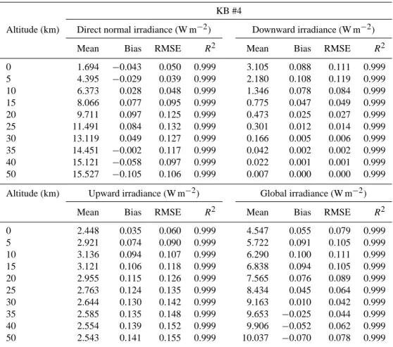
mini-Table 4. Statistical indicators of the performances of the new parameterization for computing the irradiances in Kato band #4 at different altitudes above ground level. Mean is the mean irradiance obtained from the detailed spectral calculations considered as reference.

KB #4

Altitude (km) Direct normal irradiance (W m−2) Downward irradiance (W m−2)

Mean Bias RMSE R2 Mean Bias RMSE R2

0 1.694 −0.043 0.050 0.999 3.105 0.088 0.111 0.999 5 4.395 −0.029 0.039 0.999 2.180 0.108 0.119 0.999 10 6.373 0.028 0.048 0.999 1.346 0.078 0.084 0.999 15 8.066 0.077 0.095 0.999 0.775 0.047 0.049 0.999 20 9.711 0.097 0.125 0.999 0.473 0.025 0.027 0.999 25 11.491 0.084 0.132 0.999 0.301 0.012 0.014 0.999 30 13.119 0.049 0.127 0.999 0.166 0.005 0.006 0.999 35 14.451 −0.002 0.117 0.999 0.042 0.002 0.002 0.999 40 15.121 −0.058 0.097 0.999 0.022 0.001 0.001 0.999 50 15.527 −0.105 0.106 0.999 0.007 0.000 0.000 0.999

Altitude (km) Upward irradiance (W m−2) Global irradiance (W m−2)

Mean Bias RMSE R2 Mean Bias RMSE R2

0 2.448 0.035 0.060 0.999 4.547 0.055 0.079 0.999

5 2.921 0.074 0.090 0.999 5.722 0.091 0.105 0.999

10 3.136 0.094 0.107 0.999 6.290 0.100 0.111 0.999 15 3.121 0.106 0.118 0.999 6.838 0.094 0.105 0.999 20 2.955 0.115 0.126 0.999 7.565 0.076 0.089 0.999 25 2.763 0.124 0.135 0.999 8.434 0.045 0.064 0.999 30 2.644 0.130 0.142 0.999 9.163 0.010 0.042 0.999 35 2.585 0.135 0.148 0.999 9.653 −0.025 0.044 0.999 40 2.554 0.139 0.152 0.999 9.906 −0.052 0.062 0.999 50 2.543 0.141 0.155 0.999 10.037 −0.070 0.078 0.999

mum of−0.004 W m−2_{(−3 %) at the surface, then increases} with altitude up to 0.327 W m−2_{(8 %) at 35 km and suddenly} decreases down to 0.010 W m−2_{(0 %) at 50 km. The RMSE} follows a similar trend, with a minimum of 0.005 W m−2 (2 %) at altitude of 5 km, then increases up to 0.373 W m−2 (9 %) at 35 km and suddenly decreases down to 0.034 W m−2 (1 %) at 50 km. The situation is different in KB #4 where the bias and RMSE are less dependent with altitude. The bias is small and fluctuates between a minimum of−0.070 W m−2 (−1 %) at 50 km and a maximum of 0.100 W m−2 _{(2 %,} 10 km). The RMSE is fairly constant and ranges between a minimum of 0.042 W m−2_{(1 %, 30 km) and a maximum of} 0.111 W m−2_{(2 %, 10 km).}

A similar comparison was made by Wandji Nyamsi et al. (2014) with the original approach of Kato et al. (1999) but for altitudes varying between 0 and 3 km. They reported relative bias, relative RMSE and R2 for the spectral clear-ness index KT1λ of respectively−92 %, 123 % and 0.718

for KB #3 and−16 %, 17 % and 0.991 for KB #4. For the new parameterization, with altitudes in the range [0, 3] km, the same quantities are respectively−2 %, 4 % and 0.999 for KB #3 and−2 %, 3 % and 0.999 for KB #4. The new

param-eterization improves considerably the irradiances estimated in KB #3 and KB #4.

7 Conclusions

Acknowledgements. The authors thank the teams developing

libRadtran (http://www.libradtran.org) and SMARTS and the referees whose remarks helped to improve the content of the article. This work was partly funded by the French Agency ADEME in charge of energy (grant no. 1105C0028, 2011-2016) and took place within the Task 46 Solar Resource Assessment and Forecasting of the Solar Heating and Cooling programme of the International Energy Agency. W. Wandji Nyamsi has benefited from a personal grant of the Foundation MINES ParisTech for a 3-month visit to the Finnish Meteorological Institute.

Edited by: S. Kazadzis

References

Gueymard, C.: SMARTS2, Simple model of the atmospheric ra-diative transfer of sunshine: algorithms and performance assess-ment, Report FSEC-PF-270-95, Florida Solar Center, Cocoa, FL., USA, 78 pp., 1995.

Gueymard, C.: The sun’s total and the spectral irradiance for solar energy applications and solar radiations models, Sol. Energy, 76, 423–452, 2004.

Kato, S., Ackerman, T., Mather, J., and Clothiaux, E.: The k -distribution method and correlated-k approximation for short-wave radiative transfer model, J. Quant. Spectrosc. Radiat. Transf., 62, 109–121, 1999.

ground level in clear-sky conditions, Atmos. Meas. Tech., 6, 2403–2418, doi:10.5194/amt-6-2403-2013, 2013.

Mayer, B. and Kylling, A.: Technical note: The libRadtran soft-ware package for radiative transfer calculations – description and examples of use, Atmos. Chem. Phys., 5, 1855–1877, doi:10.5194/acp-5-1855-2005, 2005.

Molina, L. T. and Molina, M. J.: Absolute absorption cross sections of ozone in the 185- to 350-nm wavelength range, J. Geophys. Res., 91, 14501–14508, 1986.

Oumbe, A., Qu, Z., Blanc, P., Lefèvre, M., Wald, L., and Cros, S.: Decoupling the effects of clear atmosphere and clouds to sim-plify calculations of the broadband solar irradiance at ground level, Geosci. Model Dev., 7, 1661–1669, doi:10.5194/gmd-7-1661-2014, 2014.

Wandji Nyamsi, W., Espinar, B., Blanc, P., and Wald, L.: How close to detailed spectral calculations is the k-distribution method and correlated-k approximation of Kato et al. (1999) in each spectral interval?, Meteorol. Z., 23, 547–556, doi:10.1127/metz/2014/0607, 2014.