Retrieval of near-surface sulfur dioxide (SO<sub>2</sub>) concentrations at a global scale using IASI satellite observations

(1)

AMTD

8, 11029–11075, 2015

Global SO2 satellite

observations

S. Bauduin et al.

Title Page

Abstract Introduction

Conclusions References

Tables Figures

◭ ◮

Back Close

Full Screen / Esc

Printer-friendly Version

Interactive Discussion

Discussion

P

a

per

|

Discussion

P

a

per

|

Discussion

P

a

per

|

Discussion

P

a

per

|

Atmos. Meas. Tech. Discuss., 8, 11029–11075, 2015 www.atmos-meas-tech-discuss.net/8/11029/2015/ doi:10.5194/amtd-8-11029-2015

This discussion paper is/has been under review for the journal Atmospheric Measurement Techniques (AMT). Please refer to the corresponding final paper in AMT if available.

Retrieval of near-surface sulfur dioxide

(SO

₂

) concentrations at a global scale

using IASI satellite observations

S. Bauduin1, L. Clarisse1, J. Hadji-Lazaro2, N. Theys3, C. Clerbaux1,2, and P.-F. Coheur1

1

Spectroscopie de l’Atmosphère, Service de Chimie Quantique et Photophysique, Université Libre de Bruxelles (ULB), Brussels, Belgium

2

Sorbonne Universités, UPMC Univ. Paris 06, Université Versailles St-Quentin, CNRS/INSU, LATMOS-IPSL, Paris, France

3

Belgian Institute for Space Aeronomy (BIRA-IASB), Brussels, Belgium

Received: 25 August 2015 – Accepted: 30 September 2015 – Published: 26 October 2015

Correspondence to: S. Bauduin ([email protected])

(2)

AMTD

8, 11029–11075, 2015

observations

S. Bauduin et al.

Title Page

Tables Figures

◭ ◮

Back Close

Full Screen / Esc

Discussion

P

a

per

|

Discussion

P

a

per

|

Discussion

P

a

per

|

Discussion

P

a

per

|

Abstract

SO2from volcanic eruptions is now operationally monitored from space in both

ultravi-olet (UV) and thermal infrared (TIR) spectral range, but anthropogenic SO2has almost

solely been measured from UV sounders. Indeed, TIR instruments are well-known to have a poor sensitivity to the boundary layer (PBL), due to generally low thermal

con-5

trast (TC) between the ground and the air above it. Recent studies have demonstrated the capability of the Infrared Atmospheric Sounding Interferometer (IASI) to measure near-surface SO2 locally, for specific atmospheric conditions. In this work, we develop

a retrieval method allowing the inference of SO2near-surface concentrations from IASI

measurements at a global scale. This method consists of two steps. Both are based

10

on the computation of radiance indexes representing the strength of the SO2 ν3 band

in IASI spectra. The first step allows retrieving the peak altitude of SO2 and

select-ing near-surface SO₂. In the second step, 0–4 km columns of SO₂ are inferred using a look-up table (LUT) approach. Using this new retrieval method, we obtain the first global distribution of near-surface SO2 from IASI-A, and identify the dominant

anthro-15

pogenic hotspot sources and volcanic degassing. The 7-year daily time evolution of SO2 columns above two industrial source areas (Beijing in China and Sar Cheshmeh

in Iran) is investigated and correlated to the seasonal variations of the parameters that drive the IASI sensitivity to the PBL composition. Apart from TC, we show that humidity is the most important parameter which determines IR sensitivity to near-surface SO2.

20

As IASI provides twice daily global measurements, the differences between the re-trieved columns for the morning and evening orbits are investigated. This paper finally presents a first intercomparison of the measured 0–4 km columns with an independent iterative retrieval method and with observations of the Ozone Monitoring Instrument (OMI).

(3)

AMTD

8, 11029–11075, 2015

observations

S. Bauduin et al.

Title Page

Tables Figures

◭ ◮

Back Close

Full Screen / Esc

Discussion

P

a

per

|

Discussion

P

a

per

|

Discussion

P

a

per

|

Discussion

P

a

per

|

1 Introduction

Sulfur dioxide (SO2) is an atmospheric trace gas with both natural and anthropogenic

sources. Volcanic emissions are the largest natural contributors to tropospheric and stratospheric SO₂, and account for 7.5–10.5 Tg of S per year on average (Andres and Kasgnoc, 1998; Halmer et al., 2002). Anthropogenic sources emit on average 60–

5

100 Tg of S per year (Stevenson et al., 2003), with the major contribution coming from combustion of sulfur-rich fuels, such as coal and oil, and smelting of heavy metals (Smith et al., 2011). The sinks of SO2are dry (Wesely, 2007) and wet (Ali-Khodja and

Kebabi, 1998) deposition, and oxidation by the OH radical in the gas phase or by O3

and H₂O₂in the aqueous phase (Eisinger and Burrows, 1998; Stevenson et al., 2003).

10

The SO2 lifetime varies according to the sinks from a few hours to several days (Lee

et al., 2011).

SO₂ emissions of most volcanoes are now well monitored from space, especially eruptive degassing. Significant amounts of SO2 are in this case mainly injected in the

high troposphere or stratosphere and cover large areas. In the ultraviolet (UV),

re-15

trievals of volcanic SO₂ have started in 1978 with the TOMS (Total Ozone Mapping Spectrometer) instrument (Krueger, 1983; Carn et al., 2003) and have continued since then with GOME (Global Ozone Monitoring Experiment) (Eisinger and Burrows, 1998), SCIAMACHY (SCanning Imaging Absorption spectroMeter for Atmospheric CHartog-raphY) (Lee et al., 2008), GOME-2 (Rix et al., 2009) and OMI (Ozone Monitoring

In-20

strument) (Krotkov et al., 2006). In the thermal infrared (TIR), volcanic SO2has been

measured from multi-channel instruments with moderate resolution (e.g. Realmuto and Watson, 2001; Watson et al., 2004) and later with high-spectral resolution instruments such as TES (Tropospheric Emission Spectrometer) (Clerbaux et al., 2008), AIRS (At-mospheric Infrared Sounder) (Carn et al., 2005) and IASI (Infrared At(At-mospheric

Sound-25

ing Interferometer) (Clarisse et al., 2008).

In contrast to volcanoes, SO2 pollution from anthropogenic activities is difficult to

(4)

meth-AMTD

8, 11029–11075, 2015

observations

S. Bauduin et al.

Title Page

Tables Figures

◭ ◮

Back Close

Full Screen / Esc

Discussion

P

a

per

|

Discussion

P

a

per

|

Discussion

P

a

per

|

Discussion

P

a

per

|

ods have successfully been developed to retrieve surface SO₂. These are included in different global products such as the operational planetary boundary layer (PBL) OMI SO2product (Krotkov et al., 2006, 2008) or the recent OMI algorithm based on a

multi-windows DOAS (Differential Optical Absorption Spectroscopy) scheme developed by Theys et al. (2015). The latter will be used for comparison purposes later in this

pa-5

per. The availability of the satellite-derived columns from the UV nadir sounders have allowed inferring SO₂ anthropogenic emissions (e.g. Carn et al., 2007; Fioletov et al., 2011, 2013, 2015; McLinden et al., 2012, 2014). This has not yet been possible from TIR instruments, which suffer from lower sensitivity to the near-surface atmosphere due to generally low temperature differences between the surface and the PBL atmosphere

10

(hereafter called thermal contrast). Recently Bauduin et al. (2014) and Boynard et al. (2014) have nevertheless demonstrated the capability of IASI to measure near-surface SO2 locally. Both studies revealed that the presence of large thermal inversions

(as-sociated to high negative thermal contrasts) and low humidity (preventing opacity in theν3band) have allowed retrieving near-surface SO2. However, the detection of SO2

15

by IASI could theoretically be achieved in other situations, particularly in case of large positive thermal contrasts, which correspond to a surface much hotter than the atmo-sphere. This is demonstrated and discussed in Sect. 3, which provides the first global distributions of near-surface SO2 from IASI over the period 2008–2014. The method

used to retrieve SO₂ columns, described thoroughly in Sect. 2, relies on the

calcula-20

tion of a hyperspectral radiance index (HRI), similarly to the work of Van Damme et al. (2014) for ammonia (NH3). As the aim of this work consists of retrieving near-surface

SO₂, the determination of the altitude of SO₂ defines the first step of the method and relies on the work of Clarisse et al. (2014). It is used to remove all plumes located above 4 km of height, which likely correspond to volcanic eruptions. The retrieval of 0–

25

4 km SO₂columns is performed in a second step, where calculated HRI are converted into columns using a look-up tables (LUT) approach. This calculation is performed us-ing only the ν3 band spectral region (1300–1410 cm−

1

(5)

AMTD

8, 11029–11075, 2015

observations

S. Bauduin et al.

Title Page

Tables Figures

◭ ◮

Back Close

Full Screen / Esc

Discussion

P

a

per

|

Discussion

P

a

per

|

Discussion

P

a

per

|

Discussion

P

a

per

|

band (around 1100–1200 cm−1_{) is not considered in this work. The whole procedure is}

described in Sect. 2.

2 SO2near-surface product

2.1 IASI and methodology

The IASI instrument is a Michelson interferometer onboard MetOp platforms (A and B)

5

circling the Earth on a Sun synchronous polar orbit. The IASI effective field of view is composed of 2_×2 footprints of 12 km diameter each at nadir. IASI has a global cover-age twice a day thanks to a swath of 2200 km and two overpasses per day (morning at 09:30 and evening at 21:30 LT at the equator). The instrument covers the thermal in-frared spectral range from 645 to 2760 cm−1_{with a spectral resolution of 0.5 cm}−1_after

10

apodization. Each measurement consists of 8461 radiance channels (0.25 cm−1

sam-pling) and is characterized by a noise of 0.2 K on average. Details about the instrument can be found elsewhere (Clerbaux et al., 2009; Hilton et al., 2012). Only measurements of the IASI-A instrument have been considered here.

The methodology used in this work to retrieve near-surface SO2 amount relies on

15

the sensitive detection method of trace gases introduced by Walker et al. (2011), and used later by Van Damme et al. (2014) for retrieving NH₃columns at global scale from IASI. Retrieval approaches based on spectral fitting generally consist of simultaneous iterative adjustments of the atmospheric parameters of interest (here the 0–4 km SO2

column) and spectrally interfering unknown variables. The idea of the proposed method

20

is to consider the interfering variables as permanent unknowns and to incorporate them in a generalized noise covariance matrixS. This matrix should include all variability coming from the parameters a_ffecting the IASI spectrum in the spectral range under consideration (here 1300–1410 cm−1_{corresponding to the}_ν

3band) but not SO2. In this

way, instead of iteratively adjusting the SO2 columns and the interfering parameters,

(6)

AMTD

8, 11029–11075, 2015

observations

S. Bauduin et al.

Title Page

Tables Figures

◭ ◮

Back Close

Full Screen / Esc

Discussion

P

a

per

|

Discussion

P

a

per

|

Discussion

P

a

per

|

Discussion

P

a

per

|

a normalized radiance index is calculated according to:

HRI=K

T S−1_(y

−y)

p

KTS−1_K

, (1)

where K is a Jacobian, a derivative of the IASI spectrum y with respect to SO₂, y is the mean background spectrum with no detectable SO2associated with the matrix

S. This matrix S acts as a weight in the projection of the observed spectrum onto

5

SO₂signature, giving more importance to IASI channels less influenced by interfering parameters. Practically,y and Sare built from a sufficiently large sample of SO2-free

IASI spectra to include the global atmospheric variability in the absence of SO2 (see

Sects. 2.2 and 2.3).

The HRI, which is unitless, can be seen as an index of detection, whose value

rep-10

resents the strength of the SO2 signal in the IASI radiance spectrum, which is related

to the amount of SO₂ in the atmosphere. The larger its value, the more likely is the enhancement of the gas. An ensemble of SO2-free spectra has a mean HRI of 0 and

a standard deviation of 1, and a HRI of 3 (which corresponds to 3σ) can reasonably be considered as the limit of detection. Because the HRI does not correspond to the

15

real column of SO2, it is therefore needed to convert it in a subsequent step. This can

be done by using look-up tables built from forward model simulations, which link the simulated HRI values to known SO₂ columns. Prior to this, as this work focuses on near-surface pollution, we use the algorithm of Clarisse et al. (2014) to select the spec-tra with detectable low altitude SO2 enhancements. Only plumes located below 4 km

20

(7)

AMTD

8, 11029–11075, 2015

observations

S. Bauduin et al.

Title Page

Tables Figures

◭ ◮

Back Close

Full Screen / Esc

Discussion

P

a

per

|

Discussion

P

a

per

|

Discussion

P

a

per

|

Discussion

P

a

per

|

2.2 Retrieval of the altitude of the plume

The altitude of SO2is retrieved using the algorithm presented in Clarisse et al. (2014).

In short, a HRI is computed for different altitudes following:

HRI(h)=K

T hS−

1

(y₋y)

q

KT_hS−1_K

h

, (2)

where theK_h is the Jacobian for SO2 located at an altitudeh. If there is a detectable

5

amount of SO₂, the function HRI(h) will peak at the altitude of the plume. Indeed, the overlap between the IASI spectrum and the SO2spectral signature is maximal at this

altitude. The height determination therefore consists in calculating the function HRI(h) and finding the altitude of its maximum.

To this end, JacobiansK_hhave been pre-calculated with the finite difference method

10

for the spectral range 1300–1410 cm−1 _{using monthly averaged H}

2O and

tempera-ture profiles in 10◦

×20◦boxes. These averages were calculated from the meteorologi-cal fields from the EUMETSAT L2 Product Processing Facility (PPF) (Schlüssel et al., 2005; August et al., 2012) using the 15 of each month of 2009, 2011 and 2013. One set of 30 vectorsK_hhas been generated for each box and for each month, considering

15

1 km thick layer of 5 DU (1 Dobson Unit=2.69_×1016molecules cm−2_{) of SO}

2, located

every 1 km from 1 to 30 km. For each IASI observation, local Jacobians are then cal-culated using a bilinear interpolation of the four closest grid boxes, to better take into account the variation of the atmospheric conditions when observations move away from the center of the boxes. The mean background spectrumy and the associated

20

covariance matrixSneeded to calculate the HRI (Eq. 2) have been built using a sam-ple of one million randomly chosen IASI spectra. Those with detectable SO2have been

filtered out using an iterative approach: first, spectra with observable SO₂ signatures were rejected using a brightness temperature difference method (see Clarisse et al., 2008, for details) and a first estimate of the matrixSis made. The second step uses

(8)

AMTD

8, 11029–11075, 2015

observations

S. Bauduin et al.

Title Page

Tables Figures

◭ ◮

Back Close

Full Screen / Esc

Discussion

P

a

per

|

Discussion

P

a

per

|

Discussion

P

a

per

|

Discussion

P

a

per

|

this initial matrix to exclude spectra with measurable HRI from the remaining set of measurements (a similar method is used in Van Damme et al., 2014; Clarisse et al., 2013). Similarly to the Jacobians,yandSare calculated over the spectral range 1300– 1410 cm−1_.

As explained in Clarisse et al. (2014), because of the use of averaged Jacobians,

5

the retrieved altitude can be biased, especially close to the surface. The best accuracy is achieved between 5 and 15 km, and the altitude estimate is provided within 1–2 km. Below 5 km, the retrieved altitude is more uncertain. However, this is not an important issue here as the altitude is used only to filter out SO2 plumes emitted by volcanoes

directly in the free troposphere. In the following, only plumes located between the

sur-10

face and 4 km above ground are selected. The retrieved SO₂corresponds therefore to a 4 km thick layer (hereafter called 0–4 km column).

2.3 Retrieval of near-surface SO2concentrations – Look-up tables

For the low SO₂ plumes, the next step consists in computing an HRI (according to Eq. 1) for each IASI measurement and converting it to a SO2 column. Different

Ja-15

cobian, y and S have been built for this second step (see section below). Because a constant Jacobian is used in the calculation of the HRI, there are several param-eters that impact its value in addition to the SO₂ abundance itself and they need to be accounted for. We have considered the impact of viewing angle (by building angle-dependent matrices for the HRI calculation; see Sect. 2.3.1) and the one of humidity

20

and thermal contrast, which are separate entries in the look-up-tables (Sect. 2.3.2).

2.3.1 Angular dependency

The dependence of the signal strength on the viewing angle has to be taken account in the conversion of HRI values. As reported by Van Damme et al. (2014), the application of a cosine factor to account for the increased path length tends to overcorrect the HRI

25

(9)

AMTD

8, 11029–11075, 2015

observations

S. Bauduin et al.

Title Page

Tables Figures

◭ ◮

Back Close

Full Screen / Esc

Discussion

P

a

per

|

Discussion

P

a

per

|

Discussion

P

a

per

|

Discussion

P

a

per

|

have been used. Specifically, between 0◦ _{and 55}◦_{, 5}◦ _{angle bins have been defined}

and a last one of 4◦_{is considered for 55–59}◦_{(IASI zenith angle ranges between 0}◦_and

58.8◦_{). For the median angle of each bin, a Jacobian has been generated for a standard}

atmosphere (Anderson et al., 1986), with a scaling factor applied to the methane profile according to Bauduin et al. (2014). A thermal contrast of 10 K has been considered. All

5

K have been calculated with the finite difference method for 200 ppb SO2 well-mixed

between 4 and 5 km, and over the 1300–1410 cm−1 _{range. For} _y _and _S _{almost the}

totality of cloud-free (i.e. cloud fraction below 20 % and available Eumetsat L2 surface temperature, atmospheric temperature and H2O profiles) observations of the 15 of

each month of 2009 and 2011 have been used, sorted by angle bins. Measurements

10

with detectable SO2have been filtered as above. In this way, for each angle bin,y and

Shave been calculated from about 750 000 spectra.

2.3.2 Look-up tables

The conversion of the HRI into SO2 column is done using look-up tables, which, as

fory andS, have been separated per angle bin. The LUTs include 4 dimensions

link-15

ing thermal contrast, total column of water, HRI and SO2 column. To build the LUT,

forward simulations of IASI spectra have been performed for a series of situations, summarized in Table 1, using the line-by-line Atmosphit software (Coheur et al., 2005). More specifically the following parameters were varied to provide a representative set of atmospheric conditions:

20

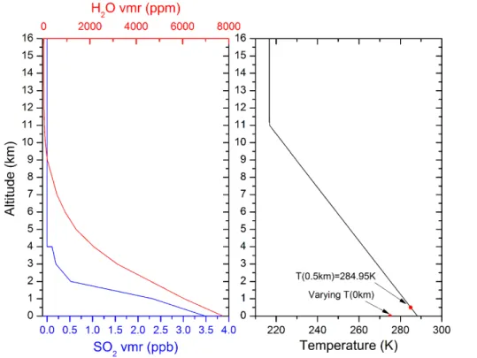
SO₂columns: To obtain a reference SO₂vertical profile for anthropogenic emissions, we relied on global chemistry transport MOZART model (Emmons et al., 2010) outputs of January, April, July and October 2009 and 2010. An average profile was calculated from all modeled profiles above Eastern United States, Europe and Eastern China, with the SO2concentration above 4 km set to zero. The resulting reference profile is shown

25

in Fig. 1 (blue). The set of atmospheric SO2 columns included in the LUT was then

(10)

AMTD

8, 11029–11075, 2015

observations

S. Bauduin et al.

Title Page

Tables Figures

◭ ◮

Back Close

Full Screen / Esc

Discussion

P

a

per

|

Discussion

P

a

per

|

Discussion

P

a

per

|

Discussion

P

a

per

|

H₂O: In a similar way, the water vapor profile from the US Standard model (Fig. 1 in red) has also been varied using 16 scaling factors (Table 1), covering a range of H2O

total column from 9.5×1019 to 2.3×1023molecules cm−2.

Temperature: A single temperature profile has been used (US standard, Fig. 1 right). To include a range of thermal contrast values, which are defined as the di_fference

5

between the temperature of the ground and the temperature of the air at 500 m (see Fig. 1), we have varied the surface temperature to provide 25 different situations, listed in Table 1. These include extreme cases of thermal contrasts, from₋30 to₊40 K, but also a range of low and moderate values. Note that a thermal contrast of 0 corresponds to an isothermal 0–1 km layer and implies that the outgoing radiance of this layer is that

10

of a blackbody (Bauduin et al., 2014). Note also that a constant emissivity of 0.98 has been used in the forward simulations. The emissivity can indeed be shown to be almost constant over the spectral range considered, but also temporally and spatially (Zhou et al., 2013).

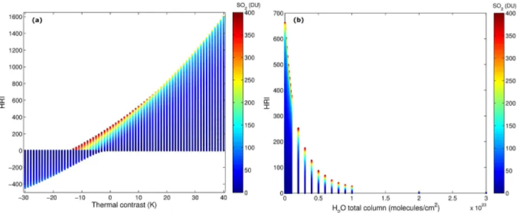
The LUTs constructed as described above have been interpolated on a finer grid

15

(TC, H2O and SO2 dimensions). An example of resulting LUT is shown in Fig. 2a (for

constant water vapor) and 2b (for constant thermal contrast). The retrieval scheme consists in determining for each IASI measurement the satellite zenith angle, the HRI, the thermal contrast, the total column of water vapor and, using the LUT, the 0–4 km column of SO₂.

20

From Fig. 2, it can be seen that the HRI has the same sign as thermal contrast. In case of positive thermal contrast, this is explained by the fact that SO2 spectral

lines are in absorption in IASI measurements, resulting in a negative difference (y₋y). Given the fact that the Jacobians are also negative (see definition in Sect. 2.3.1), the calculated HRI is positive. As a rule, for constant zenith angle, column of H2O and

25

SO₂, the value of the HRI increases with the thermal contrast. This increase in spectral signal corresponds to an increase of IASI sensitivity to near-surface SO2. However

(11)

AMTD

8, 11029–11075, 2015

observations

S. Bauduin et al.

Title Page

Tables Figures

◭ ◮

Back Close

Full Screen / Esc

Discussion

P

a

per

|

Discussion

P

a

per

|

Discussion

P

a

per

|

Discussion

P

a

per

|

HRI for constant SO₂columns, thermal contrast and viewing angle. In case of negative thermal contrast, SO2 lines are in emission and the calculated HRI is negative too.

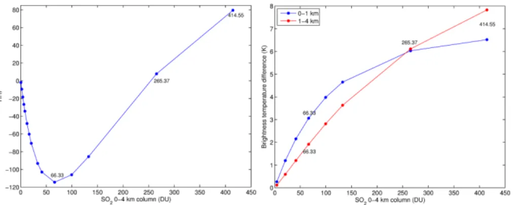
For decreasing negative thermal contrast, the HRI value usually decreases. But from Fig. 2a it can be seen that some HRI values are positive for negative thermal contrasts. We explored this seemingly odd behavior with the help of Fig. 3 (left), which shows

5

HRI as a function of SO2 for a thermal contrast of −10 K and a total column of H2O

of 2.4×1020molecules cm−2. From 0 to 66.33 DU, HRI decreases for increasing SO2.

Above 66.33 DU, the HRI starts to increase with increasing SO₂. From about 250 DU, the HRI becomes positive. This behavior can be explained by the competition between emission (mainly in the 0–1 km layer) and absorption (above 1 km). Figure 3 (right)

10

presents the contributions (in absolute value) of the emission in the 0–1 km layer and the absorption in the 1–4 km layer to the total spectral signal as function of the 0–4 km SO2 column. They have been evaluated at 1355 cm−

1

using similar techniques as in Clarisse et al. (2010). In Fig. 3, for columns ranging from 0 to 66.33 DU, emission in the 0–1 km layer increases more rapidly than absorption in the 1–4 km layer. This results in

15

decreasing HRI (more and more negative). From 66.33 DU, emission comes closer to saturation; its increase is slower than the one of absorption, whose saturation occurs for larger SO2columns, and the HRI begins to increase. From around 250 DU, absorption

totally counterbalances emission and HRI values become positive. This competition between emission in the lowest layers and absorption higher up depends on the value

20

of the temperature inversion, as the latter determines the strength of the emission. Note that this competition also depends on the altitude of the thermal inversion, but which is here constant (just above the ground). The consequence is that, for negative thermal contrast, a negative HRI can be converted into two SO2columns (see Fig. 3,

left): a small one (emission combined with lower absorption above 1 km) and a large

25

(12)

AMTD

8, 11029–11075, 2015

observations

S. Bauduin et al.

Title Page

Tables Figures

◭ ◮

Back Close

Full Screen / Esc

Discussion

P

a

per

|

Discussion

P

a

per

|

Discussion

P

a

per

|

Discussion

P

a

per

|

that the large columns for which the HRI is positive for negative thermal contrast have been kept.

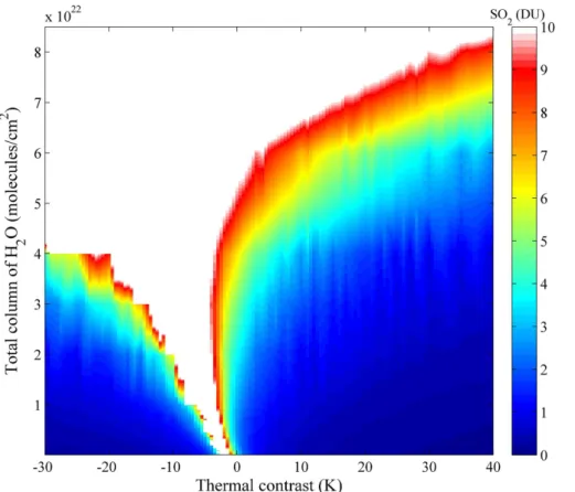
From the LUT, we can estimate the detection limit of IASI to near-surface SO2. In

Fig. 4, the lowest detectable 0–4 km column of SO₂is presented as function of thermal contrast and the total column of H2O. These columns have been calculated using the

5

LUT assuming a detection threshold of 3 on the value of HRI (see Sect. 2.1). As ex-pected, this limit of detection largely depends on thermal contrast and humidity. Indeed, when the former is close to 0, IASI stays insensitive even to large SO2 columns. For

large thermal contrasts, 0–4 km columns lower than 1 DU can be measured. This also depends on the humidity. Below 2_×1022molecules cm−2_{, the limit of detection stays}

10

below 2 DU for both high positive and high negative thermal contrasts. For larger H₂O amount, this limit rapidly increases for negative thermal contrast but stays relatively low for large positive thermal contrasts. From above 4×1022molecules cm−2 of H2O, the

detection threshold starts to increase for positive thermal contrasts.

2.3.3 Error characterization

15

To each LUT, an associated table of errors has been generated by propagating the uncertainties of the different LUT parameters:

σSO₂ = s

_∂_SO

2 ∂TC

2 σ_TC2 +

_∂_SO

2 ∂H2O

2 σ_H2

2O+

_∂_SO

2 ∂HRI

2

σ_HRI2 , (3)

whereσSO₂ is the absolute error of the SO2 column, σTC and σH₂O are the errors on

thermal contrast and total column of water vapor, which are respectively taken equal

20

to√2 K and 10 % relying on early validation of the IASI level 2 meteorological fields from the PPF (Pougatchev et al., 2009);σHRIis the standard deviation of the HRI and

is equal to 1.

An example of an error table is given in Fig. 5 for the angle bin 0–5◦ _{and for a total}

column of water vapor of 2_×1020molecules cm−2_{. As expected, the errors are directly}

(13)

AMTD

8, 11029–11075, 2015

observations

S. Bauduin et al.

Title Page

Tables Figures

◭ ◮

Back Close

Full Screen / Esc

Discussion

P

a

per

|

Discussion

P

a

per

|

Discussion

P

a

per

|

Discussion

P

a

per

|

linked to the IASI sensitivity to near-surface SO₂, with large errors (above 100 %) oc-curring in case of small thermal contrasts. The errors decrease with increasing thermal contrasts and drop to 20 % or less in the most favorable situations. As discussed above, for large total columns of H₂O, IASI is also less sensitive to near-surface SO₂and er-rors increase accordingly. The erer-rors are used in the following to filter out the data in the

5

distributions and time series and only the retrieved columns for which the conditions of surface sensitivity are fulfilled are used.

3 Results

3.1 Global distributions

The SO2 retrievals have been performed on 7 years of IASI observations (1

Jan-10

uary 2008–30 September 2014). In Fig. 6, an average global distribution of the near-surface column of SO₂ for this period is presented, separately for day (top) and night (bottom) observations. Only measurements with less than 20 % cloud fraction in the IASI field-of-view and with available surface temperature, profiles of temperature and H₂O from the EUMETSAT IASI level 2 PPF have been used. Furthermore, only

re-15

trieved SO2 columns with less than 25 % relative error and less than 10 DU absolute

error are used. The second criterion was necessary to remove spurious data over the cold Antarctic region. The columns that pass these posterior filters have been averaged on a 0.5◦

×0.5◦ grid for cells including more than 5 IASI measurements. The bottom-right inset in the daytime map presents the global anthropogenic

emis-20

sions (in kg s−1_m−2_{) of SO}

2provided by the EDGAR v4.2 inventory (downloaded from

the ETHER/ECCAD database) (EDGAR-Emission Database for Global Atmos. Res., 2011).

Figure 6 reveals several anthropogenic and volcanic hotspots, numbered from 1 to 13. Most of them are observed during the morning overpass, when the thermal contrast

25

(14)

AMTD

8, 11029–11075, 2015

observations

S. Bauduin et al.

Title Page

Tables Figures

◭ ◮

Back Close

Full Screen / Esc

Discussion

P

a

per

|

Discussion

P

a

per

|

Discussion

P

a

per

|

Discussion

P

a

per

|

1. China: China is one of the world’s largest emission sources of SO₂, mainly due to energy supply through coal combustion (Lu et al., 2010; Smith et al., 2011; Lin et al., 2012). A large region of enhanced SO2 columns, from 1 to 8 DU on the

7 year average, is seen over the industrial area surrounding Beijing. The largest columns are found close to Beijing, where emissions are the largest according to

5

EDGAR database, and then decrease westwards.

2. Norilsk: Located above the Polar Circle, Norilsk is an industrial area where heavy metals are extracted from sulfide ores. It is also well-known for its extremely high levels of pollution (Blacksmith Institutes, 2007), and more particularly for its emis-sions of SO2 (AMAP, 1998, 2006). The Norilsk smelters are also observed with

10

IASI in Fig. 6, with averaged SO₂columns varying between 1 and 9 DU. A com-parison between measurements obtained in this work and those retrieved using an optimal estimation method (Bauduin et al., 2014) is given in Sect. 3.4.1.

3. South Africa: In Fig. 6, large SO₂ columns are observed close to Johannesburg in South Africa, with averaged columns around 3 DU for daytime measurements.

15

Emissions of about 5×10−11kg s−1m−2 are reported in the EDGAR database in this area, which correspond to power plants of the Mpumalanga Highveld indus-trial region (Josipovic et al., 2009).

4. Iran: Several SO2 sources are observed above Iran. Columns of 1 to 4 DU are

measured above the smelters of Sar Cheshmeh copper complex (Rastmanesh

20

et al., 2010, 2011). Emissions of oil industries located on the Khark Island (Ardestani and Shafie-Pour, 2009; Fioletov et al., 2013) are also observed, with columns around 1 to 2 DU.

5. Balkhash: In Fig. 6, we can see that IASI is able to measure SO2above the region

of copper smelters located in Balkhash, Kazakhstan (Nadirov et al., 2013; Fioletov

25

(15)

AMTD

8, 11029–11075, 2015

observations

S. Bauduin et al.

Title Page

Tables Figures

◭ ◮

Back Close

Full Screen / Esc

Discussion

P

a

per

|

Discussion

P

a

per

|

Discussion

P

a

per

|

Discussion

P

a

per

|

6. Mexico and Popocatepetl: Columns reaching more than 10 DU are measured in the region of Mexico City and are regularly detected. These can be attributed to low altitude plume released by the Popocatepetl volcano (Varley and Taran, 2003; Grutter et al., 2008) and/or to SO₂emissions of the Tula industrial complex, located northward to Mexico City (De Foy et al., 2009). The proximity of these two

5

sources does not however allow separating their individual contribution by using only IASI observations.

7. Kamchatka volcanoes: SO₂ columns of about 2–3 DU are observed above the Kamchatka region. These probably correspond to the activity of different volca-noes located in this region (e.g. Kearney et al. (2008); see also the archive of the

10

Global Volcanism Program: http://volcano.si.edu/).

8. Nyiragongo: Above the Democratic republic of the Congo, a plume with columns larger than 10 DU is detected. It corresponds to SO2 volcanic degassing from

Nyiragongo (Carn et al., 2013) and also probably to emissions of its neighbor, the Nyamuragira (Campion, 2014).

15

9. Etna: In Fig. 6, the Mount Etna is covered by SO2, with 0–4 km columns around

6 DU. This volcano is known for its periodic degassing activity and lava fountaining events (Tamburello et al., 2013; Ganci et al., 2012).

10. Andes: A large SO2plume, with columns around 2–3 DU, is observed in the region

of the Andes and can have several origins, which are difficult to distinguish. In the

20

South of Peru, some volcanoes showed activity in the last years (e.g. Ubinas or Sabancaya, see the archive of the Global Volcanism Program: http://volcano.si. edu/). Copper smelters are located in Ilo (Carn et al., 2007), close to the coast, but are southern of the observed plume. SO2measured above Bolivia and Chile can

originate from active volcanoes of the central Andean volcanic zone (Tassi et al.,

25

(16)

AMTD

8, 11029–11075, 2015

observations

S. Bauduin et al.

Title Page

Tables Figures

◭ ◮

Back Close

Full Screen / Esc

Discussion

P

a

per

|

Discussion

P

a

per

|

Discussion

P

a

per

|

Discussion

P

a

per

|

by the EDGAR database. The presence of an artefact in this region, due to the difficulty to represent the emissivity, can however not be totally rejected. Finally, SO2measured above Argentina, Ecuador and Colombia is mainly emitted by local

volcanoes (Global volcanism Program, http://volcano.si.edu/).

11. Bulgaria: A narrow plume, with SO₂ columns of about 2 DU, is observed in

Bul-5

garia. This corresponds to the Maritsa-Iztok complex of thermal power plants lo-cated close to Galabovo and Radnevo (Eisinger and Burrows, 1998; Prodanova et al., 2008).

12. Turkey: In Turkey, lignite-fired power plants are located in different regions and are known to cause air pollution in the vicinity of the complexes (Say, 2006; Vardar

10

and Yumurtaci, 2010). The emissions of these are observed by IASI, with SO2

columns around 2–3 DU.

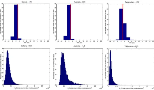
One unexpected pattern in the daytime distribution is the SO2 plume at the

ex-treme Western part of China, corresponding to the Taklamakan desert (number 13). In this region, the EDGAR inventory only documents a few of small sources but no

15

strong ones are known. While this could be explained by an artefact of the calcu-lated HRI due to sand emissivity, which strongly affects the thermal infrared measure-ments, it is noteworthy that the issue is not observed similarly above other deserts. For instance, in Fig. 7 we compare the distribution of measured HRI and the to-tal column of H2O for three desert regions: the Sahara, the center of Australia and

20

the Taklamakan. We observe that the HRI values are for almost 90 % of the cases below the detection limit of 3 above the Sahara and Australian deserts, whereas 30 % of the measurements over the Taklamakan are associated to a HRI between 3 and 5, in a few cases even above. It is therefore likely that the measured columns are real, with SO2 being transported from the source regions in East China over

25

(17)

AMTD

8, 11029–11075, 2015

observations

S. Bauduin et al.

Title Page

Tables Figures

◭ ◮

Back Close

Full Screen / Esc

Discussion

P

a

per

|

Discussion

P

a

per

|

Discussion

P

a

per

|

Discussion

P

a

per

|

make it indeed possible to measure such weak columns. Finally, the low-altitude parts of the plume released by the Nabro eruption, which followed complex transport pat-terns (Clarisse et al., 2014), are also seen during day above Ethiopia. Note that SO2is

observed above Iceland and corresponds to the Bardarbunga eruption that started in September 2014 (Schmidt et al., 2015). The different conditions and filters applied on

5

IASI measurements (see the beginning of this section) are responsible for the small-ness of the area covered by SO2.

It is worth emphasizing that some of the measured points in the 7 year average are only representative of one year. For continuous/permanent sources, this indeed depends on the inter-annual variation of thermal contrast and water vapor that limit IASI

10

sensitivity. Moreover, some particular events are typical of some years, like volcanic eruptions.

Comparison with the EDGAR database has allowed identifying observed SO2

plumes. It also points out the sources missed by IASI. Almost yearly low thermal contrasts (January–March and September–December) combined with high humidity

15

in summer (May to September) are probably responsible for the absence of Eastern United-States and Eastern Europe sources in Fig. 6. Sources in India and in South Eastern Asia are also not observed by IASI, likely because of large H₂O amount in the atmosphere in the tropical region. The problem of these missing sources is not limited to IASI. Indeed, OMI global distributions reveal the absence of some of them: South

20

Eastern Asia, part of Europe and part of India (Theys et al., 2015). These absences are possibly caused by unfavorable geophysical conditions (presence of clouds, ...), but this has to be investigated deeper. However, qualitatively, OMI and IASI global distribu-tions are in good agreement. Both instruments are able to measure large sources such as Northeast China as well as small ones, like power plants in Turkey or Bulgaria. The

25

(18)

AMTD

8, 11029–11075, 2015

observations

S. Bauduin et al.

Title Page

Tables Figures

◭ ◮

Back Close

Full Screen / Esc

Discussion

P

a

per

|

Discussion

P

a

per

|

Discussion

P

a

per

|

Discussion

P

a

per

|

When examining Fig. 6 the differences between the SO₂distributions retrieved from IASI measurements during morning (top) and evening (bottom) overpasses are also striking. In the evening distribution the plumes are more confined spatially and the columns at the center of the plumes generally larger by about a factor 3. These diff er-ences will be discussed in more details in Sect. 3.3. after the description of the time

5

series below, which brings additional clues on this difference.

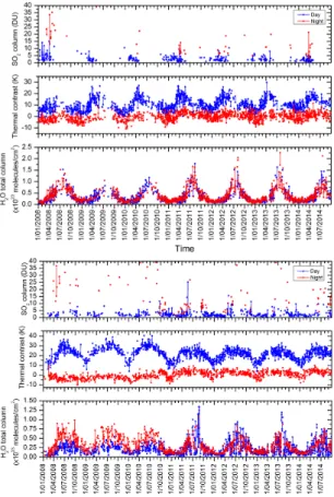
3.2 Time series

In Fig. 8, the 7 year time series (1 January 2008–30 September 2014) above Beijing and the smelters region of Sar Cheshmeh (Iran) are presented as examples. For both areas, daily averages of near-surface SO2 columns, thermal contrast and H2O total

10

column are shown, separately for the morning (blue) and evening (red) overpasses of IASI. The averages have been calculated in a circle of 125 and 75 km radius around re-spectively Beijing and Sar Cheshmeh. As before, only observations with less than 20 % cloud fraction and with available meteorological level 2 have been taken into account and only those with sufficiently low retrieval errors are considered (same thresholds as

15

before).

For Beijing and Sar Cheshmeh, the daily-averaged SO₂columns from the morning overpass vary around 3 DU, with maxima that can reach 15 DU and 25 DU respectively. The time series is incomplete for Beijing, with successful SO2retrievals from

Decem-ber to May associated with fairly high thermal contrast (10 K on average but up to 20 K;

20

Fig. 8 middle) and low humidity (below 5_×1022molecules cm−2_{; Fig. 8 bottom). The}

favorable thermal contrast conditions persist mostly year-round in Beijing but the hu-midity is too high during the other months to allow IASI probing the surface. For Sar Cheshmeh, the time series of SO₂ columns from the IASI morning overpass is more extensive and this is due to the dryness of the site as compared to Beijing (a factor 2),

25

(19)

AMTD

8, 11029–11075, 2015

observations

S. Bauduin et al.

Title Page

Tables Figures

◭ ◮

Back Close

Full Screen / Esc

Discussion

P

a

per

|

Discussion

P

a

per

|

Discussion

P

a

per

|

Discussion

P

a

per

|

It is clearly seen in Fig. 8 that IASI is mostly not sensitive to surface SO₂ above the two sites in the evening due to the drop of thermal contrast close to 0. As already noted in the previous section, the retrieved SO2columns are larger by at least a factor 3 in the

evening compared to the morning (red vs. blue symbols). This is further investigated in next section.

5

3.3 Morning-evening differences

To examine the differences in the SO2 distributions from morning and evening

over-passes, we focus hereafter on a large area (30–40◦_N_/_105–117◦_{E) above China. For}

this region and for each month in the period 1 January 2008–30 September 2014, we first calculate for morning and evening the fraction of successful SO2 retrievals, i.e.

10

those that pass the prior and posterior filters described in the previous sections and for which the HRI has a correspondence in the LUTs, relative to all the retrievals per-formed in the considered area. Regarding the last condition, it is important to point out that we found that a number of IASI measurements, mainly associated with negative thermal contrast, were not covered by the LUTs. The fraction of these measurements

15

is shown in Fig. 9 (left, second panel from top), along with the fraction of successful SO₂retrievals (top panel), as time series. They are compared (as in Fig. 8) to the time evolution of thermal contrast (third panel from top) and water content (bottom panel).

From the top panel we see that the amount of successful retrievals during the evening orbit is significantly smaller than during the morning orbit of IASI. In the morning the

20

seasonality is marked, with successful retrievals varying from close to zero in the hu-mid summer months to 20–60 % from January to May. For the evening measurements, the number of successful retrievals stays low year-round and is above 5 % only for one or two months in spring. The prime rejection criterion for the evening measurements is surprisingly the absence of correspondence, for given angles, thermal contrasts and

25

(20)

AMTD

8, 11029–11075, 2015

observations

S. Bauduin et al.

Title Page

Tables Figures

◭ ◮

Back Close

Full Screen / Esc

Discussion

P

a

per

|

Discussion

P

a

per

|

Discussion

P

a

per

|

Discussion

P

a

per

|

The fact that such situations are not included in the LUTs comes very likely from a misrepresentation of nighttime atmospheric temperature profiles and in particular temperature inversions with the conditions used to build the LUTs (Table 1). To illus-trate this, Fig. 9 (right) shows a comparison between the standard temperature profile used and a typical profile retrieved above China (35.81◦_N–117.81◦_{E) on the 29}

De-5

cember 2013. This is a situation for which the thermal contrast is−5 K and the water column 2.42_×1022molecules cm−2_{, and for which the measured HRI value of}

−3.9 has no correspondence in the LUTs. The simulation of a IASI spectrum with these two tem-perature profiles, assuming a SO2column of 4.35 DU, results in totally different values

of the HRI, +1.2 for the US Standard temperature profile and ₋4.1 for the retrieved

10

temperature profile. These results pinpoint a limitation of the current LUTs for slightly negative thermal contrast (it is not observed for large temperature inversions), which is a range where the competition between absorption and emission contributions to the HRI vary drastically. More work will be needed to avoid this shortcoming of the method in the future, either by including more temperature profiles in the calculation

15

of the LUTs or by using alternative approaches to better account for the variety of real situations encountered. Note that errors on the thermal contrast also a_ffect the HRI and, as a consequence, the retrieved SO2 column. They could be partly responsible

for the observed non correspondence between measured HRI and the LUTs.

The small number of successful retrievals in the evening measurements combined

20

with the generally lower sensitivity of IASI in this period of the day, is likely responsible in part for the factor 2–3 difference observed in the SO2columns between morning and

evening measurements. Indeed, as only the retrieved SO₂ columns with small errors are kept and as these are in the evening mainly those with large columns, the aver-ages are biased high. The effect probably also exists for the morning measurements

25

(21)

AMTD

8, 11029–11075, 2015

observations

S. Bauduin et al.

Title Page

Tables Figures

◭ ◮

Back Close

Full Screen / Esc

Discussion

P

a

per

|

Discussion

P

a

per

|

Discussion

P

a

per

|

Discussion

P

a

per

|

O₃are high, creating an important sink for SO₂, which disappears at night, favourising higher concentrations. Such a diurnal cycle of SO2 has been observed previously in

China (Wang, 2002; Wang et al., 2014) and in other regions of the world (Khemani et al., 1987; Psiloglou et al., 2013) but in others, noontime SO₂peaks have also been observed (e.g. Lin et al., 2012; Xu et al., 2014), possibly as a result of other

meteorog-5

ical/dynamical effects (Xu et al., 2014).

3.4 Product evaluation

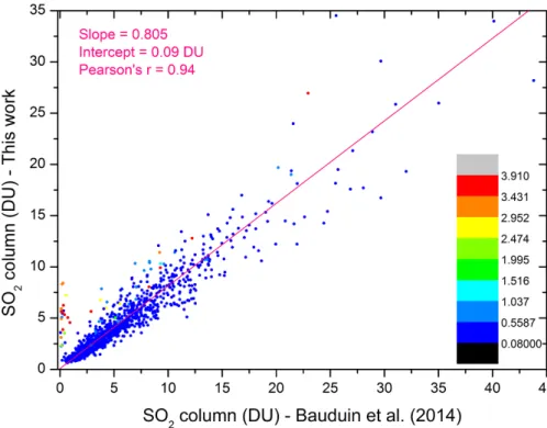
3.4.1 Comparisons with an optimal estimation retrieval scheme

As already mentioned in Sect. 3.1, Norilsk is an industrial area located in Siberia that emits large quantities of SO₂. Recently, taking the advantages of the large

tempera-10

ture inversions that develop in winter in the region, we have monitored for the first time SO2 in this area with the IASI sounder over several years (Bauduin et al., 2014), by

using a method relying on the iterative Optimal Estimation (Rodgers, 2000) and ex-ploiting a generalized spectral noise covariance matrix (see also Carboni et al., 2012). As a first assessment of the low-altitude SO2 column product developed in this work,

15

we compare the resulting 0–4 km SO₂ columns with the 0–5 km columns retrieved by Bauduin et al. (2014). The results are presented in Fig. 10. For the comparison, we consider measurements located in a circle of 150 km radius around the city of Norilsk, with less than 25 % cloud fraction, with a thermal contrast larger than 5 K in absolute value and with a humidity below 4 g kg−1 _{at 350 m above ground (this altitude}

corre-20

sponds to the average height of the temperature inversions). These last conditions ensure that near-surface SO2 is indeed probed, as explained in Bauduin et al. (2014)

and also well seen in their Fig. 3. Finally, we only consider the SO₂columns retrieved with the method described in this work with less than 25 % of relative error and less than 10 DU absolute error. The entire period 2008–2013 is analyzed, resulting in a total

25

(22)

coinci-AMTD

8, 11029–11075, 2015

observations

S. Bauduin et al.

Title Page

Tables Figures

◭ ◮

Back Close

Full Screen / Esc

Discussion

P

a

per

|

Discussion

P

a

per

|

Discussion

P

a

per

|

Discussion

P

a

per

|

dent sets of data using the reduced major axis method (Smith et al., 2009) to account for the fact that both datasets come with errors. The agreement between the columns is very good, characterized by a correlation coefficient of 0.94. The intercept, which is close to zero, and the slope of 0.80 indicate that the SO₂columns retrieved using the LUT tend to be 20 % smaller than those retrieved with the iterative method of Bauduin

5

et al. (2014). This difference is partly due to the difference in columns (0–4 km with the newly developed method against 0–5 km in Bauduin et al.) and to the difference in the profile used to build the LUTs with the a priori profile used in the iterative method. The use of the constant temperature profile for the LUTs can also cause this difference.

Finally, it is worth to emphasize in Fig. 10 the measurements for which the LUTs

10

provide a column above 2.5–3 DU and the optimal estimation retrieval a column close to 0 corresponding to the a priori column. As obvious from the color scale these retrievals are all associated with a relatively high humidity of 3 g kg−1_{. These measurements have}

a significant HRI around 5, indicating small but su_fficient signal strength, for which the iterative method has difficulties. This result shows the strength of the LUT-approach for

15

these low-signal cases.

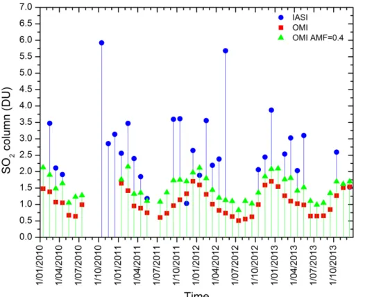
3.4.2 Comparisons with OMI derived SO2columns

OMI is an imaging spectrograph that operates in a nadir-viewing mode in the ultraviolet-visible spectral range 270–500 nm, and was launched in 2004 on the EOS-Aura NASA platform (details are given in Levelt et al., 2006). We perform a comparison of the

re-20

trieved 0–4 km SO₂column from IASI to those retrieved from OMI using the algorithm of Theys et al. (2015) for anthropogenic SO2. For the IASI column, the same filters on

cloud fraction and errors as described in Sects. 3.1 and 3.2 are applied. For the OMI columns, only those retrieved in the spectral range 312–326 nm from measurements not too much affected by the row anomaly, with solar zenith angles smaller than 65◦

25

(23)

com-AMTD

8, 11029–11075, 2015

observations

S. Bauduin et al.

Title Page

Tables Figures

◭ ◮

Back Close

Full Screen / Esc

Discussion

P

a

per

|

Discussion

P

a

per

|

Discussion

P

a

per

|

Discussion

P

a

per

|

parison in terms of a time series of the monthly averaged columns of IASI (blue) and OMI (red squares for the standard retrieval and green triangles for the retrieval using a different air mass factor (AMF)). From Fig. 11, it can be seen that the IASI columns are on average a factor 2.5 larger. The mean relative difference between the monthly averages of the two instruments is−135 % (OMI-IASI/OMI). This difference has several

5

origins. Firstly, monthly means calculated from IASI are probably overestimated by the fact that only the columns with low errors are kept, which favors the higher values of the columns. Secondly, it is likely that OMI SO2columns are underestimated. This has

al-ready been observed by Theys et al. (2015) above Xianghe (China), in the comparison with MAX-DOAS measurements (Wang et al., 2014) and explained by the

inappropri-10

ate AMF used to convert the OMI derived SO₂slant column densities (SCD) in vertical column densities (VCD). In their study, Theys et al. showed that the use of better AMF significantly improves the agreement between MAX-DOAS and OMI observations. For the sake of illustration, we also show in Fig. 11 the SO₂vertical column densities from OMI retrieved using the method of Theys et al., but with a constant AMF of 0.4, which

15

is the one used in the operational OMI PBL SO2 product (Krotkov et al., 2008). With

this correction, the agreement between the two instruments is improved; the mean relative difference becomes−65 %. Discrepancies remain but are probably within the range of what we can expect given the likely high-bias of IASI monthly averages and the di_fference in the overpass times of the two satellites.

20

4 Conclusions

In this work, we have presented a method for retrieving SO2in the low troposphere from

IASI at a global scale. The method follows two steps, both relying on the calculation of radiance indexes (HRI), which represent the strength of SO2spectral signal in IASI

measurements. In the first step, the altitude of SO2 plumes is retrieved and all plumes

25

(24)

AMTD

8, 11029–11075, 2015

observations

S. Bauduin et al.

Title Page

Tables Figures

◭ ◮

Back Close

Full Screen / Esc

Discussion

P

a

per

|

Discussion

P

a

per

|

Discussion

P

a

per

|

Discussion

P

a

per

|

4 km above it) columns using look-up tables. The construction of the LUTs is a key part of the method: it is done from forward model simulations taking into account the thermal contrast, the total column of H2O and the zenith angle. Tables of errors have

been associated with each LUT, allowing the error characterization of each retrieved SO2column and the posterior selection of the retrieved SO2columns for which IASI is

5

sensitive enough.

The method has been applied to IASI data from 1 January 2008 to 30 Septem-ber 2014 to provide global distributions and time series for the 0–4 km column. The average global distribution reveals the large known anthropogenic SO2sources, such

as the Norilsk and Sar Cheshmeh smelters, the power plants in South Africa and the

10

large industrial region in North-East China. Smaller sources, e.g. power plants in Bul-garia, are also measured. In addition to this, low altitude plumes from degassing vol-canoes are also detected. Non-negligible SO2columns have been retrieved above the

Taklamakan desert and this was explained by enhanced sensitivity of IASI in this re-gion characterized by extremely low humidity and high thermal contrast; the source

15

of the SO2 remains to be assessed. Similarly, the generally favorable conditions

oc-curring in Sar Cheshmeh (Iran) have allowed acquiring the daily time evolution of the SO2 column almost completely over the entire 7 years. This was not the case for the

Beijing area that we selected as another example region, where we show that IASI sen-sitivity has a strong seasonal cycle such that the SO₂ columns can only be retrieved

20

with small errors for the period December–May, corresponding to the driest months. The retrieved SO20–4 km columns from IASI have been compared to those of OMI on

a monthly-averaged basis. A high-bias of 135 % has been revealed, decreasing to 65 % depending on the choice of the AMF used in the OMI retrievals. More comparisons are still required to investigate deeper these observed differences. Another assessment of

25

(25)

AMTD

8, 11029–11075, 2015

observations

S. Bauduin et al.

Title Page

Tables Figures

◭ ◮

Back Close

Full Screen / Esc

Discussion

P

a

per

|

Discussion

P

a

per

|

Discussion

P

a

per

|

Discussion

P

a

per

|

considering the different assumptions and input profiles used in the two methods. This excellent agreement shows how well the new method is able to retrieve near-surface SO2. It has the advantage of being very fast; iterations and the retrieval of interfering

parameters are not needed. It is also very sensitive and has shown interestingly better results for weak SO2signals.

5

Finally, striking differences between morning and evening SO2distributions retrieved

from IASI were shown, with the SO₂columns retrieved in the evening being more con-fined spatially and larger than those from the morning by a factor 2–3. While changes in photochemistry could explain part of this effect, we have shown that it is most prob-ably due to a shortcoming with the LUT, which rely on a single temperature profile and

10

are not able to deal well with temperature inversions, which develop in the evening and in winter. Further developments will be needed to correct for this and to allow a bet-ter representativeness of the variety of temperature and humidity conditions occurring globally. The use of theν1band can also be envisaged to reduce the impact of humidity

and increase the number of used data. Despite this, given the preliminary comparisons,

15

the results obtained with this new method are however very encouraging, especially for daytime, and constitute the first successful attempt to retrieve near-surface SO₂ glob-ally with the IASI thermal infrared sensor. The continuation of this program is ensured by the soon coming launch of MetOp-C (2018) and on a longer term by the IASI-NG mission onboard MetOp-SG (Crevoisier et al., 2014).

20

Acknowledgements. IASI has been developed and built under the responsibility of the Cen-tre National d’Etudes Spatiales (CNES, France). It is flown on board the MetOp satellites as part of the EUMETSAT Polar System. The IASI L1 data are received through the EUMET-Cast near real-time data distribution service. The research in Belgium was funded by the F.R.S-FNRS, the Belgian State Federal Office for Scientific, Technical, and Cultural Affairs,

25

and the European Space Agency (ESA-Prodex arrangements). Financial support by the “Ac-tions de Recherche Concertée” (Communauté Française de Belgique) is also acknowledged. S. Bauduin, L. Clarisse and P.-F. Coheur are respectively Research Fellow, Research Associate and Senior Research Associate with F.R.S.-FNRS. C. Clerbaux is grateful to CNES for scientific collaboration and financial support. We would like to thank D. Hurtmans for the development

(26)

AMTD

8, 11029–11075, 2015

observations

S. Bauduin et al.

Title Page

Tables Figures

◭ ◮

Back Close

Full Screen / Esc

Discussion

P

a

per

|

Discussion

P

a

per

|

Discussion

P

a

per

|

Discussion

P

a

per

|

of the Atmosphit software. We also acknowledge the Ether/ECCAD database for the archiving and the distribution of the EDGAR v4.2 emission inventory.

References

Ali-Khodja, H. and Kebabi, B.: Assessment of wet and dry deposition of SO₂ attributable to a sulfuric acid plant at Annaba, Algeria, Environ. Int., 24, 799–807,

doi:10.1016/s0160-5

4120(98)00059-2, 1998. 11031

Arctic Monitoring and Assessment Programme (AMAP): Acidifying Pollutants, Arctic Haze, and Acidification in the Arctic, Chap. 9, 621–659, Arctic Monitoring and Assessment Programme (AMAP), Oslo, Norway, 1998. 11042

Arctic Monitoring and Assessment Programme (AMAP): Acidifying Pollutants, Arctic Haze, and

10

Acidification in the Arctic, Arctic Monitoring and Assessment Programme (AMAP), Oslo, Nor-way, 2006. 11042

Anderson, G., Clough, S., Kneizys, F., Chetwynd, J., and E. P., S.: AFGL Atmospheric Con-stituent Profiles (0–120 km), AFGL-TR-86-0110, Environ. Res. Papers, 954, ADA175173, 1986. 11037

15

Andres, R. J. and Kasgnoc, A. D.: A time-averaged inventory of subaerial volcanic sulfur emis-sions, J. Geophys. Res., 103, 25251–25261, doi:10.1029/98jd02091, 1998. 11031

Ardestani, M. and Shafie-Pour, M.: Environmentally compatible energy resource production-consumption pattern (case study: Iran), Environ. Devel. Sustain., 11, 277–291, doi:10.1007/s10668-007-9110-7, 2009. 11042

20

August, T., Klaes, D., Schlüssel, P., Hultberg, T., Crapeau, M., Arriaga, A., O’Carroll, A., Cop-pens, D., Munro, R., and Calbet, X.: IASI on Metop-A: Operational Level 2 retrievals after five years in orbit, J. Quant. Spectrosc. Ra., 113, 1340–1371, doi:10.1016/j.jqsrt.2012.02.028, 2012. 11035

Bauduin, S., Clarisse, L., Clerbaux, C., Hurtmans, D., and Coheur, P.-F.: IASI observations

25

of sulfur dioxide (SO₂) in the boundary layer of Norilsk, J. Geophys. Res.-Atmos., 119, 4253–4263, doi:10.1002/2013JD021405, 2014. 11032, 11037, 11038, 11042, 11049, 11050, 11074

Blacksmith Institutes: The World’s Worst Polluted Places – The Top Ten of The Dirty Thirty, The Blacksmith Institutes, New York, USA, 2007. 11042