www.atmos-chem-phys.org/acp/3/1759/
Chemistry
and Physics
On the accuracy of analysed low temperatures in the stratosphere
B. M. Knudsen
Danish Meteorological Institute, Lyngbyvej 100, 2100 Copenhagen, Denmark
Received: 20 June 2003 – Published in Atmos. Chem. Phys. Discuss.: 11 August 2003 Revised: 8 October 2003 – Accepted: 10 October 2003 – Published: 16 October 2003
Abstract. The accuracy of ECMWF (European Centre for
Medium-Range Weather Forecasts) temperatures has been investigated by comparison to radiosonde temperatures. Par-ticularly, the extent of temperatures below which Polar Stratospheric Clouds (PSCs) consisting of nitric acid trihy-drate can exist (TNAT) has been studied. In the 1999/2000 winter analyses and in the 40 year reanalyses (ERA40) from the winter 1996/1997 the analysed extent agrees quite well with the radiosondes extent, whereas the 2002/2003 win-ter analyses considerably overestimate the extent from 40– 11 hPa due to a general cold bias. Close to the frost point small-scale temperature variations, which ECMWF does not catch, substantially increase the extent of these low temper-atures. Some of these small-scale variations are caused by lee-waves.
1 Introduction
Temperatures are important in many aspects of atmospheric research and many studies have investigated the accuracy of analysed temperatures (e.g. Hertzog et al., 2003, Pommerau et al., 2002, Knudsen et al., 2002, and references therein). Ozone depletion in the Polar Regions is enhanced, when PSCs form at low temperatures. Therefore, a particular inter-est has been the accuracy of such low temperatures. Knudsen (1996) and Manney et al. (1996) compared various analy-ses to radiosonde temperatures and found substantial warm biases of the analyses. Pullen and Jones (1997) compared UK Meteorological Office (MO) analyses to partially inde-pendent ozonesondes and also found a warm bias. Davies et al. (2002) showed good agreement between radiosondes and ECMWF at low temperatures and poor agreement with MO due to erroneous ozone concentrations in the model
cli-Correspondence to:B. M. Knudsen ([email protected])
matology in the winter 1999/2000 (Manney et al., 2003). Manney et al. (2003) intercompared the PSC areas calculated from various analyses and found substantial differences. The present study updates these findings to the latest ECMWF analyses and the ERA40 reanalyses and presents some new insights concerning the role of small-scale temperature vari-ations.
2 Data
2.1 ECMWF analyses
In the winter 1999/2000 ECMWF used a T319 spherical har-monical model, with 60 vertical levels up to 0.1 hPa. The spacing in the stratosphere is 1.5 km (Simmons et al., 1999) (levels used here are at or near 10, 12, 15, 19, 23, 29, 36, 44, 55, 67, 80, 96, and 113 hPa). A 4-D variational assimi-lation scheme (Rabier et al., 2000) is used. The analyses are extracted from T106 truncated spherical harmonical fields. In the winter 2002/2003 ECMWF used a T511 truncation. On 22 January 2002, ECMWF introduced model changes concerning the assimilation of high resolution Advanced Mi-crowave Sounding Unit (AMSU) data, which significantly increased the number of data in the Arctic.
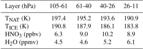
Table 1.TNAT, TICE, HNO3and H2O mixing ratios used
Layer (hPa) 105-61 61-40 40-26 26-11
TNAT(K) 197.4 195.2 193.6 190.9 TICE(K) 190.8 187.9 186.1 183.8 HNO3(ppbv) 6.3 9.0 10.2 8.9 H2O (ppmv) 4.5 4.6 5.2 6.1
ozone mixing ratios may have caused a cooling. The pe-riod 14–21 December 1995 is omitted due to excessive er-rors caused by almost no radiosondes reaching 30 hPa in the Arctic.
2.2 Radiosondes
In this study November-March radiosondes from 50◦–90◦N, and 140◦W–140◦E are used, because this is where most PSC’s occur (Pawson et al., 1995). Only 0 and 12:00 UT son-des are used. Radiosonde temperatures are reported on stan-dard levels, of which 10, 20, 30, 50, 70, 100, and 150 hPa are used here together with significant levels in between. The sondes have been taken from the ECMWF GTS archives, and only the uncorrected data are used. For consistency primarily Vaisala radiosondes have been used, although the Russian sondes perform very well at night (Luers and Es-keridge, 1998). Mainly sondes inside the polar vortex, de-fined as where MPV (modified potential vorticity referenced to 475 K; Lait, 1994) is larger than 35×10−6K m2s−1kg−1, have been used. The Vaisala radiosondes have a reproducibil-ity of 0.2 K and small IR/solar radiation corrections. Accord-ing to WMO (1998), the Canadian sondes used the radiation correction V93 and most other stations with Vaisala sondes used the V86 correction by the beginning of 1998. The V86 correction leads to approximately 0.3 K higher temperatures at 30 hPa (0.7 K at 10 hPa) during night.
In the winter 2002/2003 the Vaisala radiosonde type RS90 was used occasionally by several European and Greenland stations. Its temperature sensor has a much faster response than the one used in the RS80 radiosonde, which could lead to differences in the temperature measured, when there is a vertical gradient in the temperature.
2.3 Filtering out atmospheric waves
Atmospheric waves have a great influence on stratospheric temperatures. To determine the amount of wave activity the procedure by Whiteway (1999) has been adopted. Therefore, the temperature perturbations from a background state (a cubic polynomial fit to the radiosonde temperature profile) were calculated. The perturbation potential energy density,
Ep, was determined as the variance of fractional perturba-tion multiplied by 1/2 (g/N)2, where g is the acceleration of gravity and N is the buoyancy frequency (Whiteway,
1999). Ep was calculated in the pressure range 150–50 hPa (12–19 km), whereas Whiteway (1999) used 11–18 km. The amount of wave activity was then classified in the following way:
Ep<1 J/kg: inhibited wave activity
Ep>2 J/kg: enhanced wave activity
This procedure does not work for waves with wave-lengths longer than 7 km in the vertical, but such long waves would usually be accompanied by waves of shorter wavelengths (e.g. D¨ornbrack et al., 2002), because the mountains themselves usually have structures on a broad range of scales. However, a few strong lee-wave events with long wavelengths and temperatures close to the frost point have been re-classified as enhanced wave activity. The vertical resolution at ECMWF is 1.5 km, so waves with wavelengths shorter than 3 km cannot possibly be resolved. In most of this study only data with inhibited wave activity have been used.
3 Results
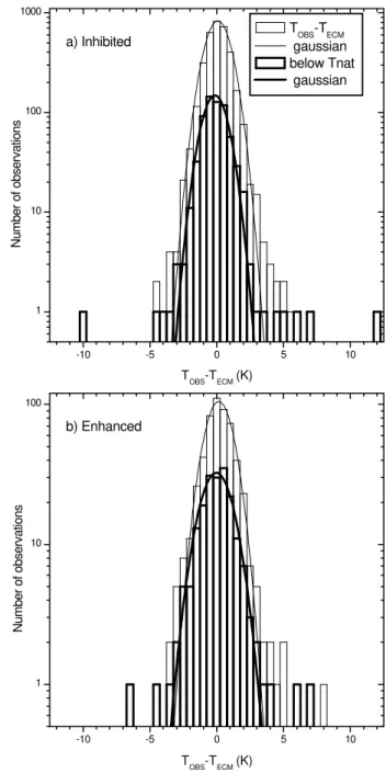
In Table 2 the median biases (TOBS-TECM) and 68% frtiles of the absolute biases are shown for inhibited wave ac-tivity for the winter 1999/2000 in the first 6 rows. The num-bers of points are given in the parentheses. From 26–11 hPa the number of ECMWF layers increases, leading to a larger number of points even though less radiosondes reach this height. The median and 68% fractile are small except for above 26 hPa, where both ECMWF and radiosonde errors be-come larger. The largest radiation corrections occur during daylight, so it is no surprise that the 68% fractile decreases for night time data as seen in row 2 of the table. However, the median is almost unchanged.
One problem with the comparison to radiosonde temper-atures is that they are assimilated into the ECMWF model together with e.g. satellite data. Therefore the ECMWF first guess, which is the 6–12 hour forecast from the previ-ous analysis, has also been used. The first guess is indepen-dent from individual radiosonde data, but a general bias of all Vaisala radiosondes could in principle be transferred to the ECMWF analyses. There is no evidence, however, that such a bias should exist as indicated by the good agreement with the results mentioned above. The weakness of the first guess field is of course that it contains forecast errors. In data sparse regions the quality of the analyses might be reduced to one comparable to that of the first guess field. This might e.g. be the case at high latitudes for the first two winters, since less AMSU data were used in the assimilation before 22 January 2002.
In row 3 the differences to the first guess field are shown. There is a substantial increase in the median of the first guess compared to the analyses above 26 hPa. Thus the ECMWF model has a cold bias, which can partially explain the pos-itive median for the analyses above 26 hPa. Other explana-tions include problems with the radiosonde temperatures due to a possible use of V86 radiations corrections for some of the radiosonde stations or a reduction of the ventilation of the temperature sensor as suggested by Luers and Eskeridge (1998). To get a feeling for the variability during the winter the February-March median for the analyses is shown in row 4, and it is evident that only minor differences occur.
In row 5 the results for temperatures below TNAT are shown. Knudsen (1996) found a substantial warm bias of the ECMWF temperatures in February and March 1996 be-low TNATfrom 125–25 hPa. The results from this study show that this bias almost vanished in 1999/2000, but as we shall see below, a substantial cold bias occurred in 2002/2003. The results for temperatures below TICE+2.5 K in row 6 indicate a warm bias of such low ECMWF temperatures at 30 hPa. To get a fair statistic one must select for occasions where ei-ther observed or modelled or both temperatures are below the given threshold temperature (Manney et al., 1996).
ECMWF temperatures have been compared to completely independent observations on long- duration balloons. The results in row 4 agree well with the results of Pommereau et al. (2002) and Knudsen et al. (2002) for a flight from 18
-10 -5 0 5 10
1 10 100 1000
a) Inhibited
Number o
f observations
TOBS-TECM (K)
TOBS-TECM gaussian below Tnat gaussian
-10 -5 0 5 10
1 10 100
b) Enhanced
Number o
f observations
TOBS-TECM (K)
Fig. 1.Histogram of the 1999/2000 temperature biases for inhibited (a)and enhanced(b)wave activity. The histograms for tempera-tures below TNATare shown in bold.
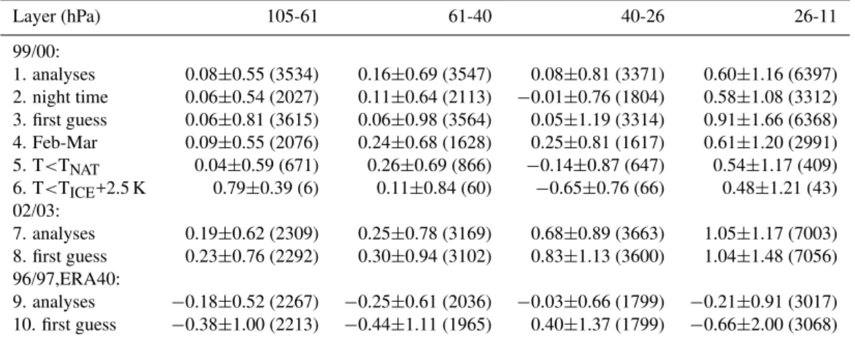
Table 2.Median temperature biases (TOBS-TECM) and 68% fractiles (K)
Layer (hPa) 105-61 61-40 40-26 26-11
99/00:
1. analyses 0.08±0.55 (3534) 0.16±0.69 (3547) 0.08±0.81 (3371) 0.60±1.16 (6397) 2. night time 0.06±0.54 (2027) 0.11±0.64 (2113) −0.01±0.76 (1804) 0.58±1.08 (3312) 3. first guess 0.06±0.81 (3615) 0.06±0.98 (3564) 0.05±1.19 (3314) 0.91±1.66 (6368) 4. Feb-Mar 0.09±0.55 (2076) 0.24±0.68 (1628) 0.25±0.81 (1617) 0.61±1.20 (2991) 5. T<TNAT 0.04±0.59 (671) 0.26±0.69 (866) −0.14±0.87 (647) 0.54±1.17 (409) 6. T<TICE+2.5 K 0.79±0.39 (6) 0.11±0.84 (60) −0.65±0.76 (66) 0.48±1.21 (43) 02/03:
7. analyses 0.19±0.62 (2309) 0.25±0.78 (3169) 0.68±0.89 (3663) 1.05±1.17 (7003) 8. first guess 0.23±0.76 (2292) 0.30±0.94 (3102) 0.83±1.13 (3600) 1.04±1.48 (7056) 96/97,ERA40:
9. analyses −0.18±0.52 (2267) −0.25±0.61 (2036) −0.03±0.66 (1799) −0.21±0.91 (3017) 10. first guess −0.38±1.00 (2213) −0.44±1.11 (1965) 0.40±1.37 (1799) −0.66±2.00 (3068)
0.8 K in good agreement with the results for the 1999/2000 winter shown here. Their standard deviations agree better with the standard deviations of the first guess field (row 3 in Table 2), which may be a more appropriate comparison.
In rows 7–10 the results for the other two winters are given. Note that in the winter 1996/1997 the number of points is smaller because the vortex formed quite late. In 2002/2003 there is a substantial bias, but a good agreement between the first guess and the analyses, whereas the oppo-site is the case in the 1996/1997 ERA40 reanalyses.
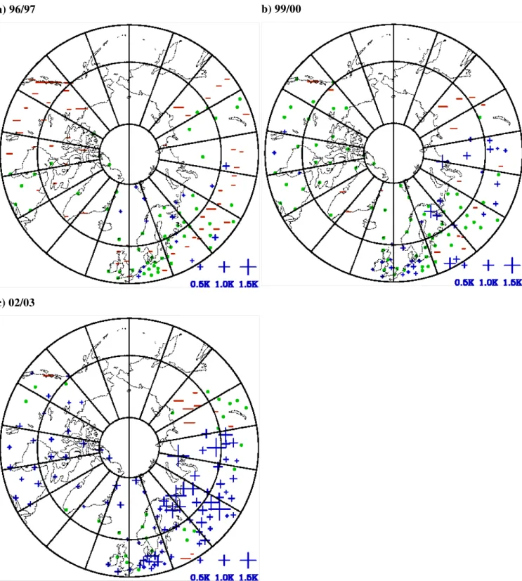
Figure 2 shows the ECMWF temperature bias during night time for all inhibited radiosondes with at least 10 observa-tions. Some of the westernmost Canadian radiosonde sta-tions use the VIZ type radiosondes, which can lead to large discrepancies if uncorrected. However, temperatures below TNATare very rare at these stations. In 1996/1997 there is (erroneously) a negative (warm) bias over the Canadian sta-tions, which could be related to their use of the Vaisala V93 radiation correction scheme. In the winter 2002/2003 there is a general positive (cold) bias, which is also present for the more accurate occasional RS90 radiosoundings. This is the only plot where Russian radiosondes and radiosondes outside the vortex have been included. The Russian son-des are included because they give an independent check on the ECMWF temperatures. The large biases over Russia in 2002/2003 may be evidence for a deteriorating Russian ra-diosonde network.
The size of the stationary anomalies found by Bowman et al. (1998) and Wagner and Bowman (2000) are not seen in the ECMWF biases. In the operational ECMWF data from 1994/1995 there are indeed signs of such large anomalies at 30 hPa (Knudsen et al., 1996). These stationary anomalies could be caused by different radiosonde types (Lait, 2002). The reason for the small ECMWF anomalies might be the radiosonde bias correction scheme implemented at ECMWF: For 4 solar zenith angle intervals the radiosonde temperatures
are corrected for the biases with respect to the first guess field for the preceding year (Onogi, 2000).
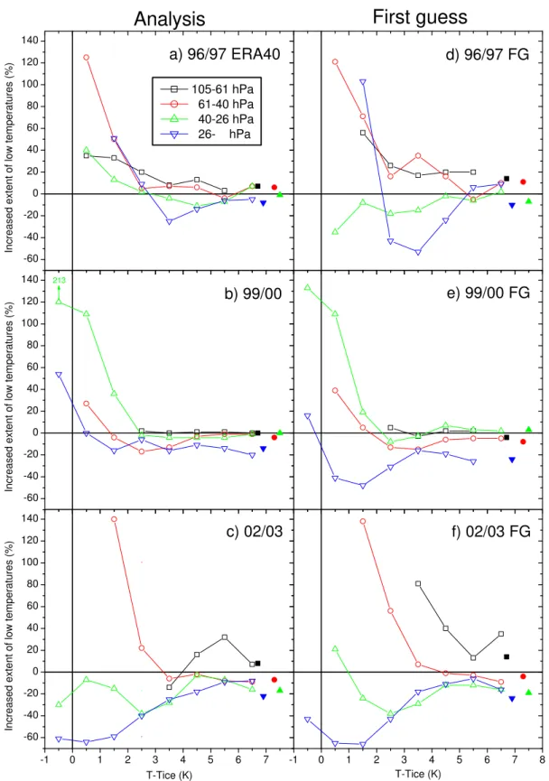
3.1 Accuracy of the PSC extent in the analyses
a) 96/97
b) 99/00
c) 02/03
-60 -40 -20 0 20 40 60 80 100 120 140
-60 -40 -20 0 20 40 60 80 100 120 140
-1 0 1 2 3 4 5 6 7
-60 -40 -20 0 20 40 60 80 100 120 140
-1 0 1 2 3 4 5 6 7 8
a) 96/97 ERA40
Increased extent of low temperatures (%)
105-61 hPa 61-40 hPa 40-26 hPa 26- hPa
213
b) 99/00
Increased extent of low temperatures (%)
c) 02/03
Increased extent of low temperatures (%)
T-Tice (K)
d) 96/97 FG
First guess
Analysis
e) 99/00 FG
f) 02/03 FG
T-Tice (K)
indicate the influence of lee-waves as described in appendix A. In the winter 2002/2003 the ECMWF temperatures have a substantial cold bias. In this winter no attempt to quantify the role of lee-waves below the frost point was made due to the uncertainties being too large. The largest effect of lee-waves is seen below the frost point, whereas for all temperatures be-low TNATlee-waves have hardly any effect (not shown). The extent of the low temperatures is always larger for the exact radiosonde temperatures than for the layer averaged temper-atures because such low tempertemper-atures are more likely to oc-cur at the temperature minimum. Small-scale temperature variations, which ECMWF does not catch, thus substantially increase the extent of temperatures close to the frost point. Some of these fluctuations are due to lee-waves. The extreme coldness in the winter 1995/1996 might explain why the frac-tion of frost point temperatures explained by lee-waves is smaller that year. It might be that the use of high- resolution radiosonde data would further increase the extent of these low temperatures in the observations. In a warm winter with small extents of temperatures below TNAT ECMWF would probably likewise substantially underestimate these extents.
D¨ornbrack and Leutbecher (2001) have shown that moun-tain waves enhance the potential for ice formation from 1980–1999 over Scandinavia in January by more than a fac-tor of two. Scandinavia, however, is not the place where temperatures below TNATmost frequently occur (Pawson et al., 1995). Our study shows a much smaller effect of moun-tain waves on the ice formation potential in agreement with Knudsen et al. (2002) and Hertzog et al. (2002). This may be explained by a bias towards mountainous regions in their results. Another explanation may be the large differences be-tween the methods used. Especially the use of four relatively cold winters in this study might influence the results, because in a warm winter synoptic temperatures may not reach the frostpoint. A complicating factor is that the ECMWF model itself does simulate some mountain waves, particularly in the 2002/2003 winter, when the horizontal resolution was high-est.
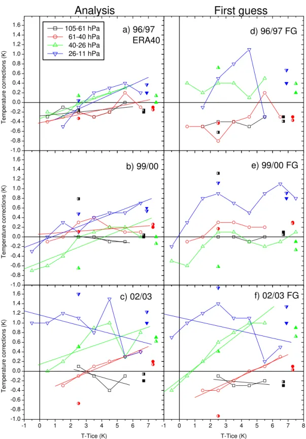
3.2 Temperature corrections
The half-filled symbols in Fig. 5 indicate the median bias (TOBS-TECM) for all temperatures below TNAT and below TICE+2.5 K. Points based on fewer than 5 observations are not plotted, whereas points based on 5–10 observations are only plotted if the 68% fractile of the absolute biases are less than 1.5 K. Figure 5 is more or less a reflection of Fig. 3. Sim-ilar to Fig. 3 the first guess biases generally have the same sign as the analysis biases, but are larger numerically. This indicates that systematic model errors play a role in the tem-perature biases of the analyses.
Other symbols in Fig. 5 show the temperature correction needed to be added to ECMWF temperatures to obtain the ra-diosonde PSC extent (without vertical averaging). This is a somewhat constructed quantity, which is not as robust against
0 2 4 6 8 10 12 14 02/03 99/00 96/97 95/96
Vertical extent (100 km)
Winter
a) Extent of T<TICE+2.5K: ECMWF
Radiosonde layer mean Radiosonde 0.0 0.5 1.0 1.5 2.0 2.5 3.0 02/03 99/00 96/97 95/96
Vertical extent (100 km)
Winter
b) Extent of T<TICE: ECMWF
Radiosonde layer mean Radiosonde
Fig. 4. Vertical extent (summed over all radiosondes) of temper-atures below TICE+2.5 K (a)and TICE (b) from 105–11 hPa for ECMWF (blue), radiosonde layer mean (green) and the exact ra-diosonde temperatures (red) for four winters. The hatched regions tentatively indicate the influence of lee-waves as described in the appendix.
radiosonde errors as the median. However, this correction is the one to apply to e.g. a chemical transport model to get the most realistic PSC extent on average through the winter. Pro-grammes to apply these temperature corrections (from the re-gression lines) to ECMWF temperatures can be downloaded from ftp://ftp.dmi.dk/pub/Ozon/ecmwftcorrections/.
In the winters 1996/1997 and 1999/2000 the temperature corrections for the analyses are small, while they are some-what larger for the first guess fields. This is particularly true in 1996/1997 and may be due to the use of a poorer model for ERA40. In the winter 2002/2003 the analysis corrections are larger, particularly above 40 hPa, but for the first guess fields the corrections are about the same. The general in-crease towards the frost point in Fig. 3 is reflected in Fig. 5 as a general decrease of the temperature corrections towards the frost point.
-1.0 -0.8 -0.6 -0.4 -0.2 0.0 0.2 0.4 0.6 0.8 1.0 1.2 1.4 1.6 -1.0 -0.8 -0.6 -0.4 -0.2 0.0 0.2 0.4 0.6 0.8 1.0 1.2 1.4 1.6
-1 0 1 2 3 4 5 6 7 8
-1 0 1 2 3 4 5 6 7
-1.0 -0.8 -0.6 -0.4 -0.2 0.0 0.2 0.4 0.6 0.8 1.0 1.2 1.4 1.6
b) 99/00
Temperature corrections (K)
a) 96/97
ERA40
Temperature corrections (K)
105-61 hPa 61-40 hPa 40-26 hPa 26-11 hPa
f) 02/03 FG
T-Tice (K)
First guess
Analysis
c) 02/03
Temperature corrections (K)
T-Tice (K)
d) 96/97 FG
e) 99/00 FG
changes in the lower stratosphere. In the ERA-40 reanalyses similar problems occur over the poles from 1998 onwards. Radiosonde errors do increase at the top levels, but such a large systematic bias is unlikely, especially during night time. Due to the 4D variational data analysis with 12 hour assim-ilation window the first guess field is a 12 hour forecast of the previous analyses in the winter 2002/2003, whereas it is a 6 h forecast in the other winters. This should increase the forecast errors, but in fact the results for the first guess field is quite similar to the results for the analyses at least in the mean.
4 Conclusions
The accuracy of ECMWF (European Centre for Medium-Range Weather Forecasts) temperatures have been investigated by comparison to radiosonde temperatures. One problem with this comparison is that the radiosonde temperatures are assimilated in the model. However, using the ECMWF first guess fields (i.e. the 6–12 hourly forecasts from the previous analyses), which are independent from the radiosonde data, gives comparable results. Below 26 hPa (40 hPa in 2002/2003) the extent of temperatures below TNAT are within 10% of the extent based on radiosondes. In the first guess fields the extent below 26 hPa is generally within 20%. Not surprisingly the largest discrepancies occurs above 26 hPa, where ECMWF fields always overestimate the extent of PSCs on average.
Appendix: Effect of lee-waves
It is not obvious how to define the effect of lee-waves on the PSC extents. The following definition is chosen: The vertical extent of temperatures below a given threshold for ECMWF, radiosonde and radiosonde mean layer tempera-tures is denotedVec,Vr, andVrm. The extent of the inhibited data has added an “i” in the subscript. The extent of the hatched (lee-wave caused) green part is defined as:
Vrm−Vrmi(Vec/Veci) (1) If this quantity is larger than the green area by an extent, x, then an extent, x, of the blue area is hatched. Thus, the blue-hatched region shows how much smaller the PSC extent would be for the radiosonde layer mean data with only inhib-ited wave activity. This occurs when ECMWF has a cold bias compared to the radiosonde layer mean temperatures at the temperature threshold. The extent of the red-hatched region is defined as:
Vr−Vri(Vrm/Vrmi) (2) In the case of 1997, where no temperatures below the frost point occur for inhibited wave activity, everything is hatched.
Acknowledgements. ECMWF is acknowledged for both their oper-ational and reanalysis data. Adrian Simmons is thanked for valuable
comments to the paper. Fruitful discussions with Andreas Stohl are gratefully acknowledged. Albert Hertzog and an anonymous ref-eree are thanked for valuable comments. The study was funded by the CEC within the MAPSCORE project.
References
Bowman, K. P., Hoppel, K., and Swinbank, R.: Stationary anoma-lies in stratospheric meteorological data sets, Geophys. Res. Lett., 25, 2429–2432, 1998.
Buss, S.: Dynamical aspects of polar stratospheric cloud forma-tion, denitrification and ozone loss, Ph.D. thesis, accepted, ETH-Z¨urich, 2003.
Davies, S., Chipperfield, M. P., Carslaw, K. S., et al.: Mod-eling the effect of denitrification on Arctic ozone deple-tion during winter 1999/2000, J. Geophys. Res., 107, 8322, 10.1029/2001JD000445, 2002.
D¨ornbrack, A. and Leutbecher, M.: Relevance of mountain waves for the formation of polar stratospheric clouds over Scandinavia: A 20 year climatology, J. Geophys. Res., 106, 1583–1593, 2001. D¨ornbrack, A., T. Birner, A. Fix, H. Flentje, A. Meister, H. Schmid, E. V. Browell, and M. J. Mahoney, Evidence for inertia gravity waves forming polar stratospheric clouds over Scandinavia. JGR 107(D20), 8287, doi:10.1029/2001JD000452, 2002.
Hertzog, A., Vial, F., D¨ornbrack, A., Eckermann, S. D., Knud-sen, B. M., and Pommereau, J.-P.: In-situ observations of grav-ity waves and comparison with numerical simulations during SOLVE/THESEO 2000 campaign, J. Geophys. Res, 107, (D20), 8292, 10.1029/2001JD001025, 2002.
Hertzog, A., Basdevant, C., Vial, F., and Mechoso, C. R.: Some results on the accuracy of stratospheric analyses in the Northern Hemisphere inferred from long-duration Balloon flights, Q. J. R. Meteorol. Soc., accepted, 2003.
Knudsen, B. M.: Accuracy of arctic stratospheric temperature anal-yses and the implications for the prediction of polar stratospheric clouds, Geophys. Res. Lett., 23, 3747–3750, 1996.
Knudsen, B. M., Pommereau, J.-P., Garnier, A., Nunes-Pinharanda, M., Denis, L., Newman, P., Letrenne, G., and Durand, M.: Accuracy of Analyzed Stratospheric Temperatures in the Win-ter Arctic Vortex from Infra Red Montgolfier Long Duration Balloon Flights, Part II: Results, J. Geophys. Res., 107(D20), 10.1029/2001JD001329, 2002.
Lait, L. R.: An alternative form for potential vorticity, J. Atm. Sci., 51, 1754–1759, 1994.
Lait, L. R.: Systematic differences between radiosonde instruments, Geophys. Res. Lett., 29(10), 10.1029/2001GL014337, 2002. Luers, J. K. and Eskeridge, R. E.: Use of radiosonde temperature
data in climate studies, J. Clim., 11, 1002–1019, 1998.
Manney, G. L., Swinbank, R., Massie, S. T., et al.: Comparison of U.K. Meteorological Office and U.S. National Meteorologi-cal Center stratospheric analyses during northern and southern winter, J. Geophys. Res., 101, 10 311–10 334, 1996.
Manney, G. L., Sabutis, J. L., Pawson, S., et al.: Lower stratospheric temperature differences between meteorological analyses in two cold Arctic winters and their impact on polar processing studies, J. Geophys. Res., 108, 11.1029/200JD001149, 2003.
Pawson, S., Naujokat, B., and Labitzke, K.: On the PSC forma-tion potential of the northern stratosphere, J. Geophys. Res., 100, 23 215–23 225, 1995.
Pommereau, J.-P., Garnier, A., Knudsen, B. M., et al.: Accu-racy of Analyzed Stratospheric Temperatures in the Winter Arc-tic Vortex from Infra Red Montgolfier Long Duration Balloon Flights, Part I: Measurements, J. Geophys. Res., 107 (D20), 10.1029/2001JD001379, 2002.
Pullen, S. and Jones, R. L.: Accuracy of temperatures from UKMO analyses of 1994/95 in the arctic winter stratosphere, Geophys. Res. Lett., 24, 845–848, 1997.
Rabier, F., Jrvinen, H., Klinker, E., Mahfouf, J.-F., and Simmons, A.: The ECMWF operational implementation of four dimen-sional variation assimilation, I: Experimental results with sim-plified physics, Q. J. R. Meteorol. Soc., 126, 1143–1170, 2000.
Schiller, C., Bauer, R., Cairo, F., et al.: Dehydration in the Arc-tic stratosphere during the SOLVE/THESEO-2000 campaigns, J. Geophys. Res., 107 (D20), 8293, doi:10.1029/2001JD000463, 2002.
Simmons, A. J., Untch, A., Jacob, C., K˚allberg, P., and Und´en, P.: Stratospheric water vapour and tropical tropopause temperatures in ECMWF analyses and multi-year simulations, Q. J. R. Mete-orol. Soc., 125, 353–386, 1999.
Simmons, A. J. and Gibson, J. K.: The 40 project plan, ERA-40 project report series No. 1, Available from ECMWF, Shinfield Park, Reading, 2000.
Wagner, R. E. and Bowman, K. P.: Wavebreaking and mixing in the Nortern Hemisphere summer stratosphere, J. Geophys. Res., 105, 24 799–24 807, 2000.
Whiteway, J. A.: Enhanced and inhibited Gravity Wave Spectra, J. Atm. Sci., 56, 1344–1351, 1999