Daytime SABER/TIMED observations of water vapor in the mesosphere: retrieval approach and first results

(1)

ACPD

9, 13943–13997, 2009

Daytime SABER/TIMED observations of water

vapor

A. G. Feofilov et al.

Title Page

Abstract Introduction

Conclusions References

Tables Figures

◭ ◮

Back Close

Full Screen / Esc

Printer-friendly Version

Interactive Discussion

Atmos. Chem. Phys. Discuss., 9, 13943–13997, 2009 www.atmos-chem-phys-discuss.net/9/13943/2009/ © Author(s) 2009. This work is distributed under the Creative Commons Attribution 3.0 License.

Atmospheric Chemistry and Physics Discussions

This discussion paper is/has been under review for the journalAtmospheric Chemistry

and Physics (ACP). Please refer to the corresponding final paper inACPif available.

Daytime SABER/TIMED observations

of water vapor in the mesosphere:

retrieval approach and first results

A. G. Feofilov1,2, A. A. Kutepov1,2, W. D. Pesnell2, R. A. Goldberg2, B. T. Marshall3, L. L. Gordley3, M. Garc´ıa-Comas4, M. L ´opez-Puertas4, R. O. Manuilova5, V. A. Yankovsky5, S. V. Petelina6, and J. M. Russell III7

1

The Catholic University of America, 620 Michigan Ave., Washington D.C. 20064, USA

2

NASA Goddard Space Flight Center, Mailcode 674, Greenbelt Rd., Greenbelt, MD 20771, USA

3

GATS Inc., 1164 Canon Blvd., Suite 101, Newport News, VA 23606, USA

4

Instituto de Astrof´ısica de Andaluc´ıa (CSIC), C/Camino Bajo de Huetor, 50, Granada 18008, Spain

5

(2)

ACPD

9, 13943–13997, 2009

vapor

Title Page

Tables Figures

◭ ◮

Back Close

Full Screen / Esc

Interactive Discussion 6

La Trobe University, Victoria, 3086, Australia

7

Hampton University, Hampton, VA 23668, USA

Received: 6 May 2009 – Accepted: 17 June 2009 – Published: 26 June 2009

Correspondence to: A. G. Feofilov (artem-feofilov@cua-nasa-gsfc.info)

(3)

ACPD

9, 13943–13997, 2009

vapor

Title Page

Tables Figures

◭ ◮

Back Close

Full Screen / Esc

Interactive Discussion Abstract

This paper describes a methodology for water vapor retrieval using 6.6 µm daytime broadband emissions measured by SABER, the limb scanning infrared radiometer

on board the TIMED satellite. Particular attention is given to accounting for the

non-local thermodynamic equilibrium (non-LTE) nature of the H2O 6.6 µm emission in

5

the mesosphere and lower thermosphere (MLT). The non-LTE H2O(ν2) vibrational level

populations responsible for this emission depend on energy exchange processes within

the H2O vibrational system as well as on interactions with vibrationally excited states of

the O2, N2, and CO2molecules. The paper analyzes current H2O non-LTE models and,

based on comparisons with the ACE-FTS satellite solar occultation measurements,

10

suggests an update to the rate coe_fficients of the three most important processes that

affect the H2O(ν2) populations in the MLT: a) the vibrational-vibrational (V–V) exchange

between the H2O and O2 molecules; b) the vibrational-translational (V–T) process of

the O₂(1) level quenching by collisions with atomic oxygen, and c) the V–T process of

the H2O(010) level quenching by collisions with N2, O2, and O. We demonstrate that

15

applying the updated H2O non-LTE model to the SABER radiances makes the retrieved

H₂O vertical profiles in 50–85 km region consistent with climatological data and model

predictions.

1 Introduction

Water vapor is one of the key components of the middle atmosphere that influences the

20

composition and energy budget of this region in a number of ways. Being a source for

chemically active constituents, such as OH, O(1D), H2, and H (Brasseur and Solomon,

2005), it participates in so called “zero-cycle” reactions where the absorption of solar

short-wave radiation leads to H2O photodissociation with subsequent recombination

in a number of processes that result in heating of the atmosphere (Sonnemann

25

(4)

ACPD

9, 13943–13997, 2009

vapor

Title Page

Tables Figures

◭ ◮

Back Close

Full Screen / Esc

rotational and vibrational transitions are small in comparison to that of CO₂ and O₃,

the water vapor concentration controls the concentration of ozone that, in turn, affects

mesospheric cooling. The long photochemical lifetime of H2O makes it an excellent

tracer for atmospheric dynamics (Peter, 1998) enabling one to follow the atmospheric

transport effects up to 80–85 km altitude. The existence of water molecules at

5

sufficiently low temperatures leads to the nucleation of ice particles in the MLT region

(e.g. Zasetsky et al., 2009). These particles are responsible for such phenomena as noctilucent clouds (NLCs) and polar mesospheric summer echoes (PMSEs, see also Appendix A for the abbreviations not explained in the text for readability’s sake). Due to high sensitivity to local kinetic temperatures, the NLC and PMSE phenomena

10

can be used as temperature probes of these regions (e.g. L ¨ubken et al., 2007) and as indicators of climate change (e.g. Thomas, 2003). NLCs have also been used as tracers of Shuttle rocket engine exhausts when an extraordinary amount of water was injected into the atmosphere causing an increase in NLC brightness (Siskind et al., 2003; Stevens et al., 2005).

15

Water vapor measurements in the MLT region have been performed since the 1970s utilizing ground- and aircraft-based microwave measurements (Croom et al., 1977; Bevilacqua et al., 1983; Hartogh et al., 1995; see also references in Brasseur and Solomon, 2005, Sect. 4.1.1). Spaceborne measurements of the water vapor altitude distributions started in 1978 with the launch of the Nimbus-7 spacecraft observatory

20

that utilized the SAMS (Drummond et al., 1980) and the LIMS (Gille et al., 1980) instruments for water vapor observations. Since then water vapor has been measured by a number of space experiments: HALOE (Russell et al., 1993), ISAMS (Taylor et al.,

1993), ATMOS (Gunson et al., 1996), CRISTA-1,2 (Offermann et al., 1999; Grossmann

et al., 2002), and others. Six satellite-borne instruments are currently performing

25

(5)

ACPD

9, 13943–13997, 2009

vapor

Title Page

Tables Figures

◭ ◮

Back Close

Full Screen / Esc

measure atmospheric emission in the limb.

Most of the methods used for inversion of infrared radiation data obtained in the limb viewing geometry are based on the solution of the radiative transfer problem under the assumption of local thermodynamic equilibrium (LTE) (Gille and Russell, 1984; Barnet,

1987). However, above about 55 km altitude the vibrational H₂O(ν2) levels, which give

5

rise to the bands providing main contribution to the 6.6 µm SABER channel, are out of LTE (L ´opez-Puertas and Taylor, 2001). As a result, water vapor density retrievals

in the MLT require solving the non-LTE problem for the populations of H₂O vibrational

levels. Non-LTE also complicates the retrieval process by making the entire problem non-local in altitudes, with the variation of the H2O density at one altitude affecting the

10

H₂O levels populations at other altitudes, especially in the MLT region. For these kinds

of tasks, the forward fitting iterative approach is preferable (Gusev, 2003) enabling one

to adjust the non-LTE populations at different altitudes to an iteratively changing profile

of the retrieved atmospheric constituent.

In this paper we describe the SABER instrument, its 6.6 µm limb emission

15

observation of the MLT (Sect. 2), and the current status of the H2O non-LTE models

(Sect. 3). Section 4 presents the computer code package ALI-ARMS and the

retrieval algorithm applied in this study. In Sect. 5 we present a sensitivity study

of the non-LTE model to the variation of a number of rate coefficients of energy

exchanges processes influencing the populations of H2O vibrational levels during

20

daytime. We demonstrate how the broadband 6.6 µm emission simulations required for the H2O density retrieval are affected by the uncertainties in available rate coefficients. Using the simultaneous common volume measurements performed by the SABER

instrument and ACE-FTS occultation experiment which is not a_ffected by non-LTE

effects we illustrate that a revision of certain rate coefficients is required for an

25

adequate interpretation of broadband 6.6 µm non-LTE H2O emissions. In this section

we describe the approach for the rate coe_fficients fitting and suggest an update to

values of these rate coefficients. In Sect. 6 we present the results of preliminary

(6)

ACPD

9, 13943–13997, 2009

vapor

Title Page

Tables Figures

◭ ◮

Back Close

Full Screen / Esc

model and show that these retrievals are in a good agreement with other observations and models. Section 7 bridges results obtained with the ALI-ARMS research code and those obtained with this code to the operational retrieval. The latter will be used

to produce H2O distributions in the next release of SABER data. This section also

describes the SABER Operational Processing Code (SOPC) that is based on the

5

GRANADA research code and discusses the retrieval uncertainties linked with the optimization of the research code for operational uses. The main results of the paper are summarized in the Sect. 8.

2 SABER instrument on the TIMED satellite

The TIMED satellite was launched on 7 December 2001 into a 74.1◦ inclined 625 km

10

orbit with a period of 1.7 h. The TIMED mission is focused on the energetics and dynamics of the mesosphere-lower thermosphere region (60–180 km) (Yee et al.,

1999). SABER, one of four instruments on TIMED, is a 10-channel broadband

limb-scanning infrared radiometer covering the spectral range from 1.27 µm to 17 µm. SABER provides vertical profiles of kinetic temperature, pressure, ozone, carbon

15

dioxide, water vapor, atomic oxygen, atomic hydrogen and volume emission rates

in the NO (5.3 µm) and OH Meinel and O₂(1∆) bands. The vertical instantaneous

field of view of the instrument is approximately 2.0 km at 60 km altitude, the vertical

sampling interval is∼0.4 km, and the atmosphere is scanned from below the surface

up to 400 km tangent height. The instrument performs one vertical scan every 53 s,

20

the scans are performed both in up- and downward directions. The latitudinal coverage

is governed by a 60-day yaw cycle that allows observations of latitudes from 83◦S to

52◦N in the South viewing phase or from 53◦S to 82◦N in the North viewing phase. The

instrument has been performing near-continuous measurements in this mode since 25 January 2002.

(7)

ACPD

9, 13943–13997, 2009

vapor

Title Page

Tables Figures

◭ ◮

Back Close

Full Screen / Esc

Interactive Discussion 3 H₂O 6.6 µm radiance measured by SABER

In the gas phase water molecule vibrations involve combinations of symmetric stretch

(ν1), covalent bond bending (ν2), and asymmetric stretch (ν3) modes with the band

strength ratio for the fundamental bands of the main H2O isotope being 0.07/1.50/1.00

for theν1,ν2, andν3vibrations, respectively (Goody and Young, 1995 and references

5

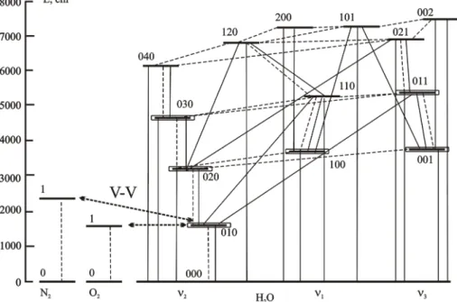
therein; Rothman et al., 2005). The diagram in Fig. 1 shows the ground and various

excited vibrational levels of H2O molecule up to 7445 cm

−1

. The levels are marked

in accordance with the number of vibrational quanta ν1ν2ν3. The 6.6 µm radiance

measured in the water vapor channel of the SABER instrument arises from the optical

transitions from vibrationally excited states with_∆ν2=1, where∆ν2denotes the change

10

in theν2vibrational quanta number.

3.1 LTE and non-LTE conditions in H₂O

The interpretation of SABER 6.6 µm limb radiance profiles requires the information

on populations of the corresponding H2O vibrational levels at the altitudes of limb

observations. In the lower atmosphere the frequency of inelastic molecular collisions

15

is sufficiently high, so that these collisions overwhelm other population/depopulation

mechanisms of the molecular vibrational levels. This leads to a local thermodynamic equilibrium, and the populations follow the Boltzmann distribution governed by the local

kinetic temperatureTkin. In the MLT, where the frequency of inelastic collisions is much

lower than that at lower altitudes, other processes also influence the population of

20

H2O vibrational levels. These include: a) the direct absorption of solar radiance by

the H2O vibrational-rotational bands in the 1.4–6.3 µm spectral region; b) absorption

of the 6.6 µm radiance coming from the warmer and denser lower atmosphere; c) vibrational-translational (V–T) energy exchanges by collisions with molecules and atoms of other atmospheric constituents; d) collisional vibrational-vibrational (V–V)

25

(8)

ACPD

9, 13943–13997, 2009

vapor

Title Page

Tables Figures

◭ ◮

Back Close

Full Screen / Esc

of kinetic and radiative transfer equations, which express the balance relations between various excitation/de-excitation processes described above.

3.2 Non-LTE model of H₂O

In this work we use two non-LTE models of water vapor developed by different groups.

The first one, with 7 vibrational levels and 10 ro-vibrational bands was developed by

5

L ´opez-Puertas et al. (1995) and updated in the book by L ´opez-Puertas and Taylor (2001). The second one, with 14 vibrational levels and 33 ro-vibrational bands was developed by Manuilova et al. (2001). The levels included in the models are shown

in Fig. 1 where the thick horizontal lines represent the vibrational levels of H₂O, O₂,

and N2 molecules while the boxed thick lines refer to the H2O levels in the model of

10

L ´opez-Puertas et al. (1995). The lowest vibrational levels of the O2and N2 molecules

coupled by V–V exchange with those of H₂O are also shown in Fig. 1. The dashed lines

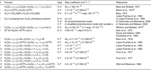
on Fig. 1 correspond to the V–V and V–T transitions listed in Table 1 (L ´opez-Puertas and Taylor, 2001; Manuilova et al., 2001). Thin solid lines show the optical transitions

between H₂O levels. Spectroscopic information for these transitions is taken from the

15

HITRAN 2004 database (Rothman et al., 2005).

In this work we concentrate on the daytime cases for two reasons. First, the

daytime 6.6 µm radiances measured by SABER are larger than the nighttime ones and

correspondingly larger SNR allows retrieving the H2O volume mixing ratio (VMR) up to

85–90 km altitude. Second, the more complicated daytime non-LTE model includes

20

the e_ffects of the nighttime model as a subset. During daytime the O₂(1) level is

populated by a complex chain of electronic-vibrational (E–V), V–V and V–T exchange

processes involving the O2/O3 photolysis products O(

1

D), O2(b 1

Σ+g, v), O2(a 1

∆g, v),

and O2(X 3

Σ−, v). The most detailed kinetics model of the O2/O3 photolysis products

was presented by Yankovsky and Manuilova (2006), hereafter YM2006. In this model

25

the quantum yield of O₂(1) molecules per O₃ photolysis event (ε) depends on the

(9)

ACPD

9, 13943–13997, 2009

vapor

Title Page

Tables Figures

◭ ◮

Back Close

Full Screen / Esc

Babaev, 2009). The model by L ´opez-Puertas and Taylor (2001) utilizes the constant

value ε=4 at all altitudes. Another aspect of coupling the system of H2O levels

with the O₂(1) level is the interaction of the latter with the second ν2 state of CO2

through V–V exchange. Depending on the season and location, this level is in non-LTE

above 70–80 km altitude and the calculation of its population requires solving the CO2

5

non-LTE problem (L ´opez-Puertas and Taylor, 2001). Besides exchanging energy with O2(v) levels, the H2O(ν2) levels interact with N2levels pumped through collisions with

the electronically excited oxygen atoms O(1D) (Zahr et al., 1975; Harris and Adams,

1983; Tachikawa et al., 1995, Edwards et al., 1996).

The non-LTE effects in populations of H2O vibrational levels for the daytime

10

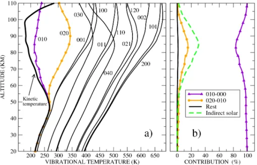
conditions in a typical atmospheric scenario are shown in Fig. 2a. The non-LTE

calculation for the case study in this plot was performed with the help of the research code ALI-ARMS (see Sect. 4 below) for mid-latitude conditions measured by the

SABER instrument (23 June 2002, lat=39.6◦N, lon=256.2◦E, solar zenith angle

θz = 79.58

◦

). The H₂O VMR profile was taken from the output of the LIMA

15

(Leibniz-Institute Middle Atmosphere) model (Sonnemann et al., 2005; Berger, 2008)

for the corresponding mid-latitude conditions. The profiles of other atmospheric

gases required for the calculations (N₂, O₂, CO₂, O, and O1D) were taken from the

corresponding SABER atmospheric model. The kinetic temperature profile and all VMR profiles were smoothed with a 4 km vertical window for demonstration purposes.

20

The populations of the levels in Fig. 2a are represented by vibrational temperatures

Tvib that describe the excitation degree of the level l against the ground level 0:

n_l/n0=gl/g0exp[−(El−E0)/k/Tvib], where El is the energy of the level l, E0 is the

energy of the ground level, k is Boltzmann’s constant, and g0, gl and n0, nl are the

degeneracies and populations of the ground andl-th levels, respectively. If the level is

25

in LTE thenTvib=Tkin. IfTvib>Tkin then the net pumping of the level is larger than that under LTE conditions. Similarly, ifTvib<Tkin, the level is populated less efficiently and/or depopulated faster than at LTE.

(10)

ACPD

9, 13943–13997, 2009

vapor

Title Page

Tables Figures

◭ ◮

Back Close

Full Screen / Esc

Fig. 1. One can see that the Tvib of different vibrational levels demonstrate different

behavior. The populations of 010 and 020 levels depart from LTE above∼55 km altitude

while levels such as 030, 100, 011, 110, 040, 021, 120, 002, 101, and 200 show the

effects of strong solar pumping down to the troposphere. The populations of the 001

and 100 levels are close to LTE below ∼45 km altitude though LTE is disturbed both

5

by weak absorption of solar radiance in line wings and by pumping from the upper levels. The contributions of various bands to the simulated SABER 6.6 µm radiance

are shown in Fig. 2b. The figure demonstrates that the fundamentalν2band (010–000

transition) dominates the 6.6 µm radiance at all altitudes with∼15–20% contribution of

the first hot band transition (020–010) in the altitude range of 60–100 km. Though there

10

is no direct contribution of the transitions from the upper vibrational levels, these levels must be included in the daytime calculations since they pump the 010 and 020 levels through a series of V–V and V–T exchanges as well as through radiative transitions. The indirect contribution of the upper levels to the daytime 6.6 µm radiance measured by SABER was calculated and put on Fig. 2b to be compared with the contributions of

15

the 010–000 and 020–010 transitions (see the dashed line in Fig. 2b). One can see that approximately 30% of the daytime signal in the SABER water vapor channel near 85 km is due to pumping the 020 and 010 levels from the upper levels.

4 ALI-ARMS research code

Most of the calculations performed in this work were made using the ALI-ARMS

20

computer code (see Kutepov et al., 1998; Gusev and Kutepov, 2003; and references therein) that solves the multi-level problem using the Accelerated Lambda Iteration (ALI) technique developed for calculating non-LTE populations of atomic and ionic levels in stellar atmospheres (Rybicki and Hummer, 1991). The code iteratively solves a set of statistical equilibrium equations and the radiative transfer equations. The

25

algorithm e_fficiency is ensured by the ALI technique, which avoids the expensive

(11)

ACPD

9, 13943–13997, 2009

vapor

Title Page

Tables Figures

◭ ◮

Back Close

Full Screen / Esc

spectral lines. The ALI-ARMS model was successfully applied by Kaufmann et al. (2002, 2003) and Gusev et al. (2006) to the non-LTE diagnostics of spectral Earth’s limb

observations from the CRISTA instrument (Offermann et al., 1999; Grossmann et al.,

2002). Kutepov et al. (2006) used this model to validate the SOPC used for temperature

retrievals from the 15 µm CO2 emissions measured by SABER. The retrieval method

5

implemented in the ALI-ARMS code is similar to that used in the SOPC, which is based on an iterative onion-peel technique using the relaxation method described in Gordley and Russell (1981). The process starts with the initial guess on a water vapor profile combined with a fixed atmospheric model (pressure, temperature, and VMRs of atmospheric gases retrieved from a corresponding SABER measurement).

10

The non-LTE populations are calculated and used for monochromatic limb radiances calculations for each limb-path that are convolved with the instrumental function for

SABER water vapor channel. The resulting simulated radianceI is compared to the

measured radiance at each tangent height, and the water vapor VMR is iterated using the following relaxation scheme: ξi+1=ξi+(Imeas−I

i

)/(∂I/∂ξ), where ξi+1 and ξi are

15

the water vapor VMRs at the i+1-th and i-th iterations, respectively, Imeas is the limb

radiance measured by SABER,Iiis the simulated limb radiance at thei-th iteration, and

(∂I/∂ξ) is the numerically calculated derivative of the radiance produced by the forward

model with respect toξ. After all limb-paths are converged, a new H2O VMR profile is

produced, and new non-LTE populations of H2O molecular levels are calculated, the

20

radiance is simulated again. The iterations are repeated until the differences between

the simulated and measured radiances become equal to the radiance noise in the channel.

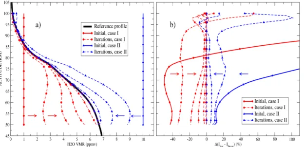
Figure 3 shows the self-consistency check of the retrieval procedure performed for the model atmosphere discussed in Sect. 3.1. First, the non-LTE task was solved for

25

the reference H2O profile, and the limb radiance was calculated using the non-LTE

populations of the H₂O levels, observation geometry, and the SABER instrumental

function. Second, the resulting radiance profile was used as the “measured” profile

(12)

ACPD

9, 13943–13997, 2009

vapor

Title Page

Tables Figures

◭ ◮

Back Close

Full Screen / Esc

equal to 1.0×10−6 (case I) and 1.0×10−5 (case II) in the 50–100 km altitude range.

Below and above this range the original values of the H2O profile were used. The

retrieval procedure was run for both cases. Figure 3a shows that the retrieved H₂O

profile rapidly converges to the reference profile in the course of iterations and that

the result does not depend on the initial profile. Figure 3b demonstrates the difference

5

between the simulated and reference radiances at each iteration. One can see that the converged radiance profile reproduces the reference profile at all points in the 50–100 km altitude range.

The described approach was tested on a number of atmospheric profiles typical

for different seasons and locations. The retrieval algorithm demonstrated the same

10

convergence stability and independence of the resulting profile on the initial guess. Potential issues with the retrieval of this kind are related to the cases where the contribution of a given tangent point to the limb-path-integrated radiance becomes small in comparison with the integrated contribution of the atmosphere lying above. This can happen if the absolute number of emitting molecules rapidly decreases

15

with altitude and the upper part of the atmosphere “blankets” the tangent point.

This scenario is realized if either the H2O VMR or vibrational levels pumping falls

rapidly with altitude. Fortunately, the H₂O VMR profiles in the Earth’s atmosphere

do not experience rapid falloffs when moving from top to bottom. To avoid the

problem of insufficient levels pumping we do not consider the nighttime cases or the

20

measurements for whichθz≥88.0

◦

.

5 Validating the non-LTE H₂O model

The accuracy of non-LTE modeling depends on the quality of the experimental and

theoretical rate coefficients describing the populating and de-populating of the H₂O

vibrational states that are listed in Sect. 3. The largest source of error in the

non-25

(13)

ACPD

9, 13943–13997, 2009

vapor

Title Page

Tables Figures

◭ ◮

Back Close

Full Screen / Esc

study performed for the H₂O non-LTE model, describe the method that was applied

to validating the set of rate coefficients used in the model, and suggest an update to

some of these coefficients.

5.1 Sensitivity study

We examined the sensitivity of H₂O(ν2) and especially the H2O(010) populations

5

to variations of V–V rates, V–T rates, and effective quantum yield ε for various

atmospheric scenarios. We also estimated the effects of temperature uncertainties

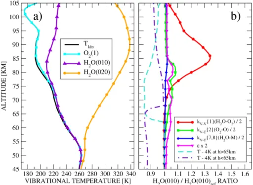
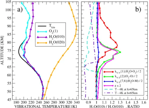
both in the LTE dominated and in the non-LTE dominated areas. Here we discuss the results for three test cases: tropical, mid-latitude winter, and polar summer (Figs. 4–6, respectively). The atmospheric pressure-temperature profiles as well as profiles of

10

other atmospheric gases, except H₂O, were taken from the current V1.07 SABER

dataset (http://saber.gats-inc.com/). The parameters of the SABER scans used for sensitivity study are: lat=1.23◦S, lon=7.24◦E, θz=26.62◦ for tropics; lat=42.14◦S, lon=11.2◦E,θ_z=64.12◦ for mid-latitude winter; lat=73.56◦N, lon=22.59◦E,θ_z=55.96◦

for polar summer. The scans were performed on days 198 and 199, 2002. The H2O

15

profiles were modeled by LIMA (Berger, 2008) for the corresponding conditions. The

left panels of Figs. 4–6 show the kinetic temperature (T_kin) distributions for considered

test cases as well as the vibrational temperatures of H₂O(010), H₂O(020), and O₂(1)

levels obtained by solving the non-LTE problem with the nominal set of rates from Table 1. The mid-latitude winter and tropical temperature profiles are characterized

20

by a moderate di_fference (∼60–70 K) between the stratopause and the mesopause.

The vibrational temperature of the H2O(010) level for these cases deviates from the

kinetic temperature in the MLT showing moderate non-LTE effects. On the other hand,

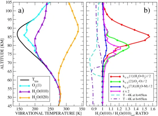
the polar summer temperature profile (Fig. 6a) has stronger temperature gradients,

and the stratopause-mesopause temperature difference is about twice as large as

25

that obtained for mid-latitude winter and tropics, which is typical for this period (She and von Zahn, 1998). The vibrational temperatures shown in Fig. 6a illustrate that

(14)

ACPD

9, 13943–13997, 2009

vapor

Title Page

Tables Figures

◭ ◮

Back Close

Full Screen / Esc

consequently, the solution of the non-LTE problem will be more sensitive to the rate

coe_fficients. Common sense supported by results shown in Figs. 4a, 5a, and 6a

suggests that one can expect the following behavior of the H2O(010) population with

respect to various rate changes: increase of the H2O(010) quenching rate must lead

to a decrease in H₂O(010) population at altitudes above 65–70 km for the tropical and

5

mid-latitude modes. This is also true for polar summer up to∼104 km altitude, where

the H2O(010) vibrational temperature crosses the kinetic temperature profile and the

e_ffect reverses. Similarly, an increase of the H₂O(010)–O₂(1) V–V rate will lead to

a more efficient de-population of the H2O(010) level and, as a result, to a H2O(010)

population decrease in the 65–95 km altitude range, with the effect depending on the

10

model. Using the same logic one can conclude that an increased O₂(1) quenching

will result in a decreased H2O(010) population and, finally, that the enhanced O2(1)

pumping will cause the H2O(010) level population to increase.

Having this in mind we tested the sensitivity of the H₂O(010) population to each

of the following processes: H2O(ν2)–O2(1), H2O(ν2)–N2(1), and O2(1)–CO2(020) V–V

15

exchanges, and H2O(ν2)–O2, H2O(ν2)–N2, H2O(ν2)–O, O2(1)–O2, O2(1)–N2, and

O₂(1)–O V–T quenching, and quantum yield ε for the O₂(1) pumping. First, we

performed a reference run for each atmospheric scenario with the rates from Table 1. Then, a series of test runs were made. For all test runs we fixed the rates in the non-LTE model except for one that was decreased to half its nominal value. We believe that for

20

the purposes of our test, the rate decrease is more representative than its increase since the latter drives the level populations closer to LTE or to LTE in a group of levels while the former “decouples” the level from the other ones and/or from LTE. We also

performed the runs with doubled quantum yieldε=8 to estimate the sensitivity of the

H2O(010) population to O2(1) level pumping. For each test run the resulting H2O(010)

25

populations at different altitudes were compared to the reference ones. The results of

the study are shown on Figs. 4b, 5b, and 6b where the ratio of H2O(010) population

(15)

ACPD

9, 13943–13997, 2009

vapor

Title Page

Tables Figures

◭ ◮

Back Close

Full Screen / Esc

processes for which halving the corresponding reaction rate leads to more than a 3%

change in the resulting H₂O(010) population for either of the model atmospheres and

for at least one altitude point. As anticipated, the polar summer case demonstrates the

largest non-LTE effects in the set of three model atmospheres. For convenience we

will refer to the processes from Table 1 using their type, number in the table, and the

5

molecules/atoms involved in the reactions: kV−V{1}(H2O−O2), kV−T{2}(H2O−M), and

so on. The highest sensitivity of the H2O(010) population and, therefore, of the 6.6 µm

radiance in the 65–100 km altitude range is tokV−V{1}(H2O−O2) and kV−T{2}(O2−O)

rate coefficients though their importance varies for different atmospheric models: in

the polar summer and tropical cases the H2O(010) population is more sensitive to

10

kV−V{1}(H2O−O2) while in the mid-latitude case the effects from kV−V{1}(H2O−O2)

and kV−T{2}(O2−O) rates, and from doubling the quantum yield, are comparable.

The combined effect of kV−T{7}(H2O−N2,O2) and kV−T{8}(H2O−O) rates is less

pronounced in all three scenarios reaching 5% only in the polar summer case.

Other parameters and factors that affect the H2O(010) population are (from most

15

to least important): kV−V{3}(O2−CO2),kV−V{5}(H2O−N2),kE−V{6}(O

1

D−N2), utilizing

the simplified photochemical pumping of O₂(1) from O₃photolysis with constant profile

of quantum yield ε, reducing the number of vibrational levels in the H2O model

from 11 to 7, and kV−T{9}(H2O−N2) through kV−T{16}(H2O−O). The small effect

of replacing the complicated scheme of O₂/O₃ photolysis product kinetics with the

20

constant quantum yield profile needs an explanation. As follows from (Manuilova et al., 2001) and (Yankovsky and Babaev, 2009) the simplified model does not provide

an accurate estimate of O2(1) pumping. However, utilizing it for the H2O non-LTE

task appears to be reasonable. As the corresponding curves in Fig. 4b, Fig. 5b,

and Fig. 6b show, the sensitivity to O2(1) pumping peaks at ∼70–80 km altitude and

25

becomes small at altitudes below∼60 km and above∼80 km. Below∼60 km the O2(1)

pumping is masked by LTE processes since any extra source is rapidly thermalized by

frequent collisions. On the other hand, O2(1) pumping above 80 km does not strongly

(16)

ACPD

9, 13943–13997, 2009

vapor

Title Page

Tables Figures

◭ ◮

Back Close

Full Screen / Esc

pressure. Therefore, one can use a fixed quantum yield model for the purposes of

H₂O VMR retrieval because this model adequately describes the quantum yield in

60–80 km altitude range while avoiding the expensive O2/O3photolysis product kinetics

calculations. For the sake of accuracy, we suggest that H2O non-LTE models replace

the constant quantum yieldε=4 with the average quantum yield profile estimated by

5

Yankovsky and Babaev, (2009). According to this work,ε=8 at 50 km altitude and falls

with the altitude increase to ε=6 at 71 km, ε=4 at 80 km, ε=1.5 at 90 km. It almost

reaches zero at 100 km altitude. This profile was used in the current study.

5.2 Sensitivity to local temperature

Apart from being sensitive to rate coefficients of various processes, the H2O(ν2)

10

populations and, consequently, radiances in the 6.6 µm channel depend on local

temperatures. Correspondingly, one has to estimate the possible e_ffects of temperature

uncertainty and bias prior to non-LTE model validation. This is of particular

importance since recent estimates performed by Remsberg et al. (2008) show

that the accuracy of the SABER temperature retrieval is about ±2 K in the upper

15

stratosphere and lower mesosphere. At the same time, SABER V1.07 temperatures (Remsberg et al., 2008; J.-H. Yee, private communications, 2009) show up to a 4 K negative bias in comparison with other measurements in the upper stratosphere

and lower mesosphere. We performed the temperature sensitivity studies for all

three atmospheric scenarios described above using the following approach. As one

20

can see from Figs. 4a, 5a, and 6a, the approximate “LTE/non-LTE threshold” for all

three atmospheric models is at∼65 km altitude. Accordingly, two test runs for each

atmosphere were made to estimate the local and non-local effects of temperature

profile variation on water vapor retrieval. First, the temperature profile was modified in accordance with the formula: Tnew(z)=Told(z)−4.0×{1−exp[−(h(z)−hthreshold)]},

25

where Tnew(z) is modified temperature value at the altitude point z, Told(z) is

unperturbed temperature,h(z) is altitude at point z in km, andhthreshold is a threshold

(17)

ACPD

9, 13943–13997, 2009

vapor

Title Page

Tables Figures

◭ ◮

Back Close

Full Screen / Esc

h(z)>hthreshold=62.0 km. The second test profile was obtained by applying the correction defined by the formula: Tnew(z)=Told(z)−4.0×{1−exp[−(hthreshold−h(z))]}for all altitudesh(z)<hthreshold=68.0 km. The results of the tests are shown on Figs. 4b, 5b, and 6b, where the temperature sensitivity curves are in agreement with the non-LTE

e_ffects plotted on Figs. 4a, 5a, and 6a. For all cases considered here decreasing

5

the temperature in the LTE area results in decreasing the H2O(010) population

at all altitude levels where the correction was made. Moreover, the sensitivity of

H₂O(010) populations in the MLT to temperature changes in the stratosphere and

lower mesosphere clearly shows that the absorption of radiance coming from below

pumps the H2O(010) levels in the MLT. On the other hand, decreasing the temperature

10

in non-LTE area has no e_ffect on the H₂O(010) population in the lower atmospheric

layers though it still affects the H2O(010) populations locally. This effect decreases

as the altitude increases and is less pronounced in the polar summer mesosphere in comparison with the tropical and mid-latitude cases. However, all three model cases

demonstrate sensitivity of the H2O(010) population and, consequently, the water vapor

15

retrieval, to kinetic temperature variations up to ∼80 km altitude. With this in mind

we can start validating the H₂O non-LTE model using a H₂O VMR dataset that was

retrieved from the measurements that are insensitive to non-LTE effects, namely, the

ACE-FTS occultation experiment.

5.3 ACE-FTS occultation measurements 20

The Atmospheric Chemistry Experiment (ACE) on the SCISAT-1 platform, is a Canadian satellite for the remote sensing of the Earth’s atmosphere that has been in operation since August 2003. The primary instrument on ACE is a Fourier-Transform

Spectrometer (FTS) with 0.02 cm−1spectral resolution. Working primarily in the solar

occultation observation mode, it provides vertical profiles of temperature, pressure,

25

and the VMRs for 18 atmospheric molecules in the 10–100 km altitude range at 4 km

vertical resolution over the latitudes 85◦S to 85◦N (Bernath et al., 2005). Trace

(18)

ACPD

9, 13943–13997, 2009

vapor

Title Page

Tables Figures

◭ ◮

Back Close

Full Screen / Esc

(∼0.3–1.0 cm−1) portions of the spectrum that contain spectral features related to

a molecule of interest with minimal spectral interference from other molecules (Boone

et al., 2005; Boone et al., 2007). One advantage of using solar occultation for

trace gases retrievals in the MLT is its independence from non-LTE issues since the instrument high spectral resolution allows tracking only the transitions from the ground

5

state whose population can be considered to be equal to the total density of the specie. Recently, the comprehensive validation of the ACE-FTS water vapor profiles (Lambert

et al., 2007; Carleer et al., 2008) has shown that the accuracy of H2O measurements

is better than 5% in the 15–70 km altitude range and is better than 10% up to 82 km altitude. This makes the ACE-FTS measurements a suitable correlative dataset for

10

comparison with SABER measurements.

5.4 SABER H₂O validation

As follows from Sect. 5.1, the H₂O(010) population and, consequently, of retrieved H₂O

concentration or VMR, are most sensitive to the rates of the following processes: H2O(ν2)–O2(1) V–V exchange, O2(1)–O V–T quenching, and H2O(ν2)–N2,O2,O V–T

15

quenching with the corresponding rate coe_fficientskV−V{1}(H2O−O2),kV−T{2}(O2−O),

and kV−T{7,8}(H2O−M). HereM stands for N2, O2, and O, while {7,8} refers to the

7-th and 8-th rows in Table 1, respectively. The measured and theoretically estimated values ofkV−V{1}(H2O−O2) andkV−T{2}(O2−O) rate coefficients are given in Table 2.

Apparently, the value of kV−V{1}(H2O−O2) rate coefficient varies by more than an

20

order of magnitude, and the largest value ofkV−T{2}(O2−O) is 2.5 times the smallest

one. The estimates for the uncertainties ofkV−T{7,8}(H2O−M) from the work of Bass

(1981) are of the same order as for thekV−T{2}(O2−O). These uncertainties require

searching for an optimal set of rates that will give the best agreement of the non-LTE measurement with reference climatologies and/or datasets.

25

(19)

ACPD

9, 13943–13997, 2009

vapor

Title Page

Tables Figures

◭ ◮

Back Close

Full Screen / Esc

measurements in different seasons and at different latitudes. The altitude distribution

of water vapor measured by ACE-FTS was taken as truth and used in a forward simulation of 6.6 µm SABER radiance. All other atmospheric parameters (temperature, pressure, VMRs of other atmospheric components) were taken from the corresponding SABER record. The calculations were performed on a grid for each of the considered

5

rates, and the resulting calculated radiances were compared with those measured

by SABER in the non-LTE region. Then the chi-square (χ2) space was searched for

a minimum (Chap. 15 in Press et al., 2002) that provided the set of rate coe_fficients that,

being applied to SABER measurements in 6.6 µm channel, gives the best agreement between SABER and ACE-FTS. The coincidences have been selected around four

10

seasonal turning points in both hemispheres in 2004 and 2005: vernal equinox, June solstice, boreal equinox, and December solstice. The total number of profiles

used for this validation was 40. The SABER data for each ACE-FTS scan was

selected based on an “overlapping weight” value estimated by the empirical formula:

γ=∆t×4+∆η×5+∆ζ×1+6/(90−θz), where ∆t is time difference between the scans

15

in h, ∆η is latitude difference in degrees, ∆ζ is longitude difference in degrees, θz

is solar zenith angle in degrees, and numbers 4, 5, 1, and 6 are the empirically

found coefficients. The scans for which at least one of the following conditions was

true: ∆t>1 h, ∆η>4◦,∆ζ >20◦,θz>89◦ were excluded from the comparison. We also

excluded the up-scan events to eliminate biases related to hysteresis effects in the

20

SABER detector. For each of the selected scans the corresponding SABER data were extracted from the V1.07 data base. The water vapor VMR profile was substituted with the coincident ACE-FTS VMR profile. All vertical profiles were interpolated onto a 1 km altitude grid.

According to Figs. 4–6, the non-LTE area is sensitive to both the local temperature

25

and the temperature variations in the stratosphere. Therefore, the temperature biases

in the atmospheric models selected for the comparison can affect the non-LTE analysis.

(20)

ACPD

9, 13943–13997, 2009

vapor

Title Page

Tables Figures

◭ ◮

Back Close

Full Screen / Esc

with temperatures measured by lidars, MIPAS, and HALOE instruments and found a 2 K negative bias in SABER temperatures in the stratopause. This bias increases

with the altitude increase and reaches −8 K at the mesopause level. Unfortunately,

the uncertainties in these biases are comparable or even larger than the biases themselves, and this does not allow using the vertical profile of the bias shown in

5

this work. On the other hand, the comparison of SABER temperatures with the

results obtained by the COSMIC GPS radio occultation experiment (J.-H. Yee, private communications, 2009) gives maximum negative deviation of 5 K in the stratopause region that decreases both in up- and downward directions. We note that neither comparison separated the upward and downward SABER scans, the former subject

10

to detector hysteresis e_ffects in the stratopause and lower mesosphere. In this work

we use the uniform temperature correction obtained from the comparison of downward SABER scans and ACE-FTS measurements. The correction can be approximated with the formulaTnew(z)=Told(z)+4.0×exp{−0.007×[59.0−h(z)]

2

}, whereTnew(z) is an

updated temperature value at an altitude z, Told(z) is the unchanged SABER V1.07

15

temperature profile, 4.0 is the maximal temperature shift in K, 0.007 is a damping

parameter, 59.0 is the altitude (in km) corresponding to a maximal temperature

shift, and h(z) is the altitude. This correction overlaps within uncertainty limits

with the corrections suggested by Remsberg et al. (2008) and J.-H. Yee (private communications, 2009) and at the same time using the bias we suggest here

20

makes the validation with ACE-FTS self-consistent. Improvements of the SABER

temperature retrieval are ongoing, and the next release of SABER data will contain updated temperature profiles that will advance the temperature-dependent retrievals of

atmospheric constituents at altitudes below∼70 km.

There were 63 rate combinations compiled from 7 values for kV−V{1}(H2O−O2)

25

rate coefficient, 3 values for kV−T{2}(O2−O), and 3 values for kV−T{7,8}(H2O−M). Each of these 63 combinations was applied to 40 tested atmospheres. For each

of 63×40=2520 cases the ALI-ARMS simulated radiance Icalc was compared to the

(21)

ACPD

9, 13943–13997, 2009

vapor

Title Page

Tables Figures

◭ ◮

Back Close

Full Screen / Esc

60 km<h(z)<85 km. The lower altitude limit of 60 km was selected because the

non-LTE e_ffects are mostly important above this altitude. The upper altitude limit

of 85 km was set because of the radiance noise level. The analysis results are

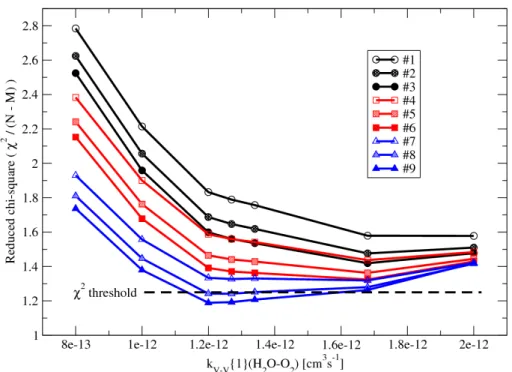
shown in Fig. 7, where the chi-square values (Press et al., 2002) are plotted. Theχ2 values were calculated using the formulaχ2=Σi ,j{[Imeas(i , j)−Icalc(i , j)]/σi ,j}2,

5

where Imeas(i , j) is 6.6 µm radiance measured by SABER, Icalc(i , j) is the radiance

calculated with the SABER atmosphere and ACE-FTS H2O VMR profile for i-th

atmospheric model atj-th altitude point, σi ,j is the signal comparison uncertainty for

the same point, and the sum is performed over all altitudes and atmospheric cases

for a given set of the rate constants. The σ_{i ,j} values were estimated using SABER

10

radiance measurement uncertainty, error of ACE-FTS water vapor measurement, and

atmospheric variability within ∆t, ∆η, and ∆ζ limits. The obtained χ2 values were

divided by (N−M) where N=1040=26×40 is the number of data points and M=3 is

the number of parameters. The obtained measure is a “reduced χ2 statistic” that

demonstrates the “goodness of fit” of the model. For a perfectly accurate model

15

the variance of [Imeas(i , j)−Icalc(i , j)] matches the σi ,j variance, and the reduced χ

2

equals one. We note that the numerical interpretation of the χ2 values should be

done with caution as the data used forχ2 calculation are not completely independent

as is required by the statistical theory. The radiances belonging to one vertical

scan are coupled through the radiative transfer between the layers. Temperature

20

sensitivity curves in Figs. 4–6 clearly show this coupling. The same effects would be

achieved by increasing the H2O VMR in the lower atmosphere. On the other hand,

increasing the H₂O VMR in the mesosphere will decrease the radiance escaping

the stratospheric area. This reasoning does not change the general approach of

a χ2 minimum search, although it does not allow the straightforward interpretation

25

of its numerical value. Since χ2 depends on three parameters, kV−V{1}(H2O−O2),

kV−T{2}(O2−O), andkV−T{7,8}(H2O−M), Fig. 7 represents a four-dimensional picture.

For simplicity we show the reduced χ2 dependencies in a form of cross-sections

(22)

ACPD

9, 13943–13997, 2009

vapor

Title Page

Tables Figures

◭ ◮

Back Close

Full Screen / Esc

lines coded by colors and symbols represent 9 combinations of 3 kV−T{2}(O2−O)

values with 3 values of kV−T{7,8}(H2O−M) rate coefficient. As follows from

Fig. 7, the minimum of χ2 is reached when k_V∗₋_V{1}(H2O−O2)=1.2×10

−12

cm3s−1, k_V∗₋_T{2}(O2−O)=3.3×10−

12

cm3s−1, andk_V∗₋_T{7,8}(H2O−M) is 1.4 times enhanced in

comparison with thekV−T{7,8}(H2O−M) rates given in Table 1. Here and below the

5

asterisk symbols denote the rate coe_fficients that yield the best correlation between

the SABER and ACE-FTS measurements. For the reasons described above we didn’t

use the [min{χ2}+1] value to define the confidence region for the rate coefficients.

Instead, we set theχ2threshold to 1.25 based on the quality of the retrieved H2O VMR

profiles. Using this threshold we obtain the following values for the rate coe_fficients:

10

k_V∗₋_V{1}(H2O−O2)=(1.2+0.4/−0.1)×10−12cm3s−1 (1)

k_V∗₋_T{2}(O2−O)=(3.3±0.7)×10−12cm3s−1 (2)

k_V∗₋_T{7,8}(H2O−M)=(1.4±0.4)×kV−T{7,8}(H2O−M) (3)

5.5 Rate coe_fficients

Comparison of the obtained rate coefficients (1)–(3) with the values given in Tables 1

15

and 2 shows that thek_V∗₋_V{1}(H2O−O2) rate coefficient retrieved from the combined

SABER and ACE-FTS data is consistent with other recent measurements and estimates of this rate (Zhou et al., 1999; Koukuli et al., 2006; L ´opez-Puertas, 2009). This result can be considered as an independent one since MIPAS measurements

were not correlated either with SABER, or with ACE. The value ofk_V∗₋_T{2}(O2−O) rate

20

coefficient supports higher values of this rate and is consistent with the measurements

(23)

ACPD

9, 13943–13997, 2009

vapor

Title Page

Tables Figures

◭ ◮

Back Close

Full Screen / Esc

Interactive Discussion 5.6 Retrieval uncertainties

The uncertainties obtained in the rate coefficients analysis were used for the error

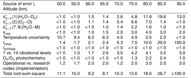
analysis in H2O VMR retrievals. Table 3 shows the single profile retrieval uncertainties

related to various aspects of measurements and retrievals, as well as the combined

retrieval error. The values in the table cells are averaged over the seasons and

5

latitudes and are given in percent of the total H2O VMR value at given altitudes.

Errors linked with three major rates uncertainties are presented in the corresponding “k_V∗₋_V{1}(H2O−O2)”, “kV∗−T{2}(O2−O)”, and “kV∗−T{7,8}(H2O−M)” rows. The “krest” row shows the combined error due to uncertainties in other rates listed in Table 1. Errors related to temperature uncertainties in SABER were estimated using the data of

10

Remsberg et al. (2008) and J.-H. Yee (private communications, 2009).Imeasin the table

refers to errors linked to the noise in radiance measurements, while an “IHITRAN” row

represents errors related to uncertainties in the HITRAN2004 spectroscopic database. The uncertainties introduced by the model simplifications discussed in Sect. 3.2 and

operational code implementations are shown in three rows. The effects of reducing

15

the vibrational levels number from 14 to 7 are listed in the “7 vs. 14 vibrational levels”

row. The “O2/O3 photochemistry” row shows the errors introduced by using a fixed

quantum yield profile for O2(1) pumping instead of a full photochemical model. The

effects introduced by the SOPC operational code are shown in the “Operational vs.

research codes (implementation)” row. This error is estimated from the comparison of

20

the SABER operational code and ALI-ARMS and GRANADA research non-LTE codes that will be discussed in Sect. 7 and Fig. 9b. As follows from Table 3, the largest

uncertainty source below ∼65 km is the temperature uncertainty which is consistent

with the sensitivity studies presented in Sect. 5. Above∼65 km and below∼80 km the

rate coefficients uncertainties dominate the total error, and above∼80 km the retrieval

25

error is mostly defined by the signal noise. Using the values from Table 3 as a guide

for a rough estimate of the absolute magnitude of H2O VMR retrieval error one will

(24)

ACPD

9, 13943–13997, 2009

vapor

Title Page

Tables Figures

◭ ◮

Back Close

Full Screen / Esc

the stratopause area and about±0.3 ppmv in the mesopause region. Armed with the

knowledge obtained in this section we now discuss H₂O retrieval from SABER data.

6 H₂O retrievals from SABER measurements

6.1 Input data

Our first non-LTE H2O retrievals from SABER measurements were performed for 4

5

atmospheric scenarios selected in 2004 and 2007: vernal equinox, June solstice, boreal equinox, and December solstice. For each case only one orbit was selected thus providing an “instantaneous snapshot” of the atmosphere for which the earliest and the latest measurements are separated by less than an hour and latitudes vary

by at least 90 degrees. As in Sect. 5.4, we chose only the downward scans to

10

eliminate the hysteresis e_ffects. The parameters of the selected scans are listed in

Table 4. The selection of days and orbits around seasonal turning points was made to obtain the best latitudinal coverage for daytime SABER measurements. The profiles of pressure, temperature, and VMRs of atmospheric gases were taken from current V1.07 SABER data available at http://saber.gats-inc.com/. The V1.07 temperature profiles

15

were modified in accordance with the approach discussed in Sect. 5.4. All the profiles were interpolated onto a 1 km vertical grid from 15 km through 135 km altitude. The

H2O retrievals were performed for the 50.0–90.0 km altitude interval. Below and above

this interval we used the corresponding H2O VMR data interpolated from ACE-FTS

measurements. The ALI-ARMS research code used for the retrievals was modified to

20

include the updated rate coefficients (1)–(3). The other rate coefficients for the non-LTE

modeling were taken from Table 1.

6.2 H₂O VMR retrievals

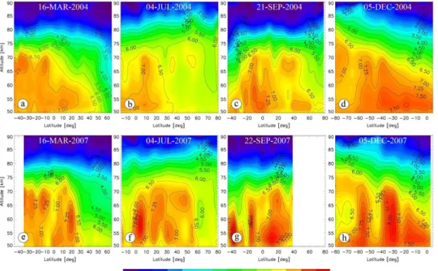
The retrieved water vapor VMRs are shown in Fig. 8a–h. The upper and lower rows refer to the years 2004 and 2007, correspondingly. The panels from left to right in

(25)

ACPD

9, 13943–13997, 2009

vapor

Title Page

Tables Figures

◭ ◮

Back Close

Full Screen / Esc

both rows represent 4 different seasons: vernal equinox, June solstice, boreal equinox,

and December solstice. The latitudinal resolution on each panel is∼6◦; the retrieved

altitudinal-latitudinal H2O VMR distributions were linearly interpolated over 1 degree

latitudinal grid and smoothed in two dimensions (3 km altitude by 2 degrees latitude

window) for demonstrational purposes. The di_fferences in the latitudinal coverage

5

on the panels are due to changes in the daytime observation geometry for different

seasons. The detailed analysis and comparisons of SABER H2O VMR distributions

with other measurements and models is the subject of a separate study and will not be done here.

6.2.1 Absolute values 10

First, we consider the minimum and maximum values that can be seen on the plotted

H₂O VMR distributions. Those minimum values that are below 0.5 ppmv define the

upper altitude limit for physically sound SABER H2O measurements, which appears to

be in the 85–90 km range depending on latitude and season. The maximum values

can be used for a rough estimate of the SABER H₂O “goodness” by comparing them

15

to other measurements. As Fig. 8d–g and especially Fig. 8h show, the largest values retrieved from SABER exceed 8.0 ppmv at altitudes around 60 km. In general, these

values seem to be overestimated compared to data from other sources. Various

measurements (Peter, 1998; Lambert et al., 2007; Nedoluha et al., 2007; Carleer

et al., 2008) show that the H2O VMR values at 60 km usually do not exceed 7.5 ppmv.

20

Occasional increases of H₂O VMR up to 7.8 ppmv at 60 km near boreal equinox were

reported by Nedoluha et al. (1996), Nedoluha et al. (1998), and Peter (1998), and were partially explained by increases in tropospheric methane emissions. Though these discrepancies are within declared accuracies of the compared datasets, we believe that they will be reduced after the SABER pressure-temperature retrieval is

25

re-analyzed, stimulated by the researches of Remsberg et al. (2008); J.-H. Yee (private communications, 2009), and this work.

(26)

ACPD

9, 13943–13997, 2009

vapor

Title Page

Tables Figures

◭ ◮

Back Close

Full Screen / Esc

H₂O VMR measured at Lauder (45◦S), at Mauna Loa (19.5◦N) by Nedoluha et al.

(2007), and at ALOMAR (69.2◦N) (Sonnemann et al., 2009). The midlatitude SABER

measurements were compared with MLS, HALOE, and WVMS (Nedoluha et al., 1997)

data while the high latitude data were compared with H₂O VMR profiles obtained

with a microwave monitoring system (Hartogh et al., 1995; Sonnemann et al., 2009).

5

As can be seen from Table 5, the H2O VMR values at 50–80 km agree well, within

the experimental uncertainties, with other measurements. High spatial and temporal variability of the atmosphere makes this result particularly encouraging. In summary,

the first analysis of the retrieved SABER H2O VMR values shows a good agreement

with other measurements taking into account the accuracy of the compared data.

10

6.2.2 Meridional structure

The retrieved water vapor distributions in Fig. 8a–h follow a known latitudinal pattern for

these seasons. The H2O VMR decrease from the summer to the winter hemisphere,

which is clearly seen in Fig. 8d,h and, to a lesser extent, in Fig. 8b,f, is explained by

vertical wind behavior in different seasons when the downward transport is increased

15

in winter and changes to the upward transport in summer (Garcia and Solomon, 1994;

K ¨orner and Sonnemann, 2001). As a result, in winter the air from above, where the H₂O

VMRs are small due to the mesospheric photochemical effects, moves down hence

drying the atmosphere. The summertime mechanism works in the opposite direction

giving rise to an increased H₂O VMR in mesosphere. Another reason for the H₂O VMR

20

decrease from the summer to the winter hemisphere is the strong pressure decrease at high latitudes in the winter hemisphere that is linked with the lower temperatures

below∼70 km altitude.

The small-scale latitudinal structures that can be seen on nearly all panels of Fig. 8 can be explained by a strong vertical wind variability discussed by K ¨orner and

25

Sonnemann (2001). Their Fig. 5b shows that wind direction changes 6 times as

the latitude varies from 60◦S to 60◦N leading to horizontal inhomogeneities in the

(27)

ACPD

9, 13943–13997, 2009

vapor

Title Page

Tables Figures

◭ ◮

Back Close

Full Screen / Esc

and 2007 (Fig. 8a,e, respectively) can be explained by larger downward transport at

high latitudes in 2007 that is seen as an abrupt change in H₂O VMR decrease at

30◦N. The same trend can be seen on Fig. 8f where well-defined horizontal structures

reveal a strong vertical wind variability, while low H2O VMR values at 10◦S indicate the

direction of vertical winds in this area. Larger peak values at heights around 60 km in

5

2007 can be explained both by larger vertical wind activity and photochemical effects.

Generally, this maximum arises due to a competition of two photochemical processes:

photodissociation of H₂O in the mesosphere and methane oxidation. The variations of

solar activity have their maximum effect on H2O VMR at heights above 65 km (Chandra

et al., 1997). Enhanced tropospheric CH4emissions give rise to increased water vapor

10

in the stratosphere and lower mesosphere. One can explain the larger absolute values

of H2O VMR in 2007 (Fig. 8e, g, and h) by a stronger vertical transport of methane from

lower atmospheric layers. The comprehensive analysis of the latitudinal and seasonal variations that will be possible with the coming new release of SABER data will reveal more information about these atmospheric phenomena.

15

7 From research to operational code

The implementation of the non-LTE H₂O model and retrieval algorithm in SOPC has

been verified using two research non-LTE codes. The ALI-ARMS code was described above. The GRANADA code (L ´opez-Puertas et al., 1995; Funke et al., 2002) uses a general-purpose non-LTE algorithm that calculates vibrational and rotational non-LTE

20

populations for relevant atmospheric IR emitters by iteratively solving the statistical equilibrium (SEE) and radiative transfer equations (RTE) with due consideration of radiative, collisional and chemical excitation processes. Internal radiation transfer is carried out with the KOPRA model (Stiller et al., 2000). The iteration scheme, i.e., the order of solutions of SEE and RTE, can be chosen by the user, allowing for Curtis

25