Mapping Individual Brain Networks Using
Statistical Similarity in Regional Morphology
from MRI
Xiang-zhen Kong1,3, Zhaoguo Liu1,3, Lijie Huang1,3, Xu Wang1,3, Zetian Yang1,3, Guangfu Zhou1,3, Zonglei Zhen1,3*, Jia Liu2,3*
1State Key Laboratory of Cognitive Neuroscience and Learning & IDG/McGovern Institute for Brain Research, Beijing Normal University, Beijing, 100875, China,2School of Psychology, Beijing Normal University, Beijing, 100875, China,3Center for Collaboration and Innovation in Brain and Learning Sciences, Beijing Normal University, Beijing, 100875, China
*[email protected](ZZ);[email protected](JL)
Abstract
Representing brain morphology as a network has the advantage that the regional morphol-ogy of‘isolated’structures can be described statistically based on graph theory. However, very few studies have investigated brain morphology from the holistic perspective of com-plex networks, particularly in individual brains. We proposed a new network framework for individual brain morphology. Technically, in the new network, nodes are defined as regions based on a brain atlas, and edges are estimated using our newly-developed inter-regional relation measure based on regional morphological distributions. This implementation allows nodes in the brain network to be functionally/anatomically homogeneous but different with respect to shape and size. We first demonstrated the new network framework in a healthy sample. Thereafter, we studied the graph-theoretical properties of the networks obtained and compared the results with previous morphological, anatomical, and functional net-works. The robustness of the method was assessed via measurement of the reliability of the network metrics using a test-retest dataset. Finally, to illustrate potential applications, the networks were used to measure age-related changes in commonly used network met-rics. Results suggest that the proposed method could provide a concise description of brain organization at a network level and be used to investigate interindividual variability in brain morphology from the perspective of complex networks. Furthermore, the method could open a new window into modeling the complexly distributed brain and facilitate the emerg-ing field of human connectomics.
Introduction
Most studies examining brain morphology have focused on local morphological features with either voxel/vertex- or region-based methods [1]. As these local features are believed to reflect clinical conditions and individual differences in various tasks [2], they have become
a11111
OPEN ACCESS
Citation:Kong X-z, Liu Z, Huang L, Wang X, Yang Z, Zhou G, et al. (2015) Mapping Individual Brain Networks Using Statistical Similarity in Regional Morphology from MRI. PLoS ONE 10(11): e0141840. doi:10.1371/journal.pone.0141840
Editor:Huiguang He, Chinese Academy of Sciences, CHINA
Received:May 5, 2015
Accepted:October 13, 2015
Published:November 4, 2015
Copyright:© 2015 Kong et al. This is an open access article distributed under the terms of the
Creative Commons Attribution License, which permits unrestricted use, distribution, and reproduction in any medium, provided the original author and source are credited.
Data Availability Statement:The dataset is publicly available from Neuroimaging Informatics Tools and Resources Clearinghouse (https://www.nitrc.org/).
Funding:This study was funded by the National Natural Science Foundation of China (31230031, 31221003, and 31470055), the National Basic Research Program of China (2014CB846101), and Changjiang Scholars Programme of China.
particularly popular as a neuroscience research topic. However, the human brain is a complex network that generates and integrates information from multiple sources [3]. In the past decade, researchers revealed some of the underlying architecture of nontrivial entities based on anatomical (e.g., through diffusion magnetic resonance imaging, dMRI) or functional net-works (e.g., through functional MRI) [4]. Given these findings, it was expected that repre-senting the brain morphology as a network would provide a holistic perspective on the understanding of the morphology of‘isolated’brain structures. For instance, with the net-work representation, researchers can obtain exclusive information reflecting an important aspect of the associations and interactions between multiple regions, which is not evident in local MRI information.
Thus far, several attempts have been made to construct morphological networks. Some researchers have proposed an approach involving estimation of interregional relationships, with covariance between averaged regional cortical thickness or gray matter (GM) volume measures across participants [5,6]. However, this method can only construct one network with a large population and is incapable of constructing an individual morphological net-work. This limits its application in the investigation of individual variability in brain struc-ture, particularly in identifying structural brain abnormalities in single patients. Comparing morphological features of different regions within individuals requires definition of corre-spondence mapping between the voxels of these regions. More recently, as a solution, Tijms et al. (2012) proposed an insightful strategy for constructing an individual morphological network. In such an approach, the entire brain is parcellated into 3 × 3 × 3 cubes (i.e., 27 voxels), and the pattern correlation between two cubes is defined as a connection. Although this approach was designed to capture the complex morphological structure of the brain, it does not take the remarkable variability in the shapes and sizes of different regions. More importantly, with such an approach, rigid extraction of the small cubes would not allow optimal correspondence with functionally or anatomically homogeneous regions of the brain [7].
To overcome the limitations mentioned above, we proposed a new network framework for individual brain morphology based on regional morphological distribution information. Tech-nically, in the new network, nodes are defined as regions based on a brain atlas, and edges are estimated using our newly-developed interregional relation measure based on regional mor-phological distributions [8]. The connection metric allows estimation of the relationship between a pair of regions with different shapes and sizes and has been found to be informative for investigating individual brain morphology with MRI scans [8]. A similar distribution-based approach has been proposed to combine cortical surface and its connecting white-matter geometry to successfully characterize individual differences in brain structure [9]. Considering these strengths, we extended our initial investigation of single morphological connections and introduced the connection metric to the research field of complex brain networks. One of the competitive advantages of the new network framework is that it allows for the construction of brain networks for a single participant, using his or her MRI scans. Thus, the method has the potential to provide a new avenue for investigating intra- and interindividual differences in brain morphology at the network level.
Materials and Methods
Participants
We used the Kirby21 dataset [10], consisting of 21 healthy adult volunteers with no history of neurological conditions (age range: 22–61 years, 10 females). Further details regarding the dataset can be found below and in Landman et al. (2011). The dataset is publicly available from Neuroimaging Informatics Tools and Resources Clearinghouse (https://www.nitrc.org/) and this study was approved by the Institutional Review Board of Beijing Normal University.
Data acquisition
Structural MRI data were all acquired via the same 3.0T scanner (Achieva, Philips Medical sys-tems) using a high-resolution 3D magnetization-prepared rapid acquisition of gradient echoes (MPRAGE; [11]) sequence with the following parameters: resolution, 1.0 × 1.0 × 1.2 mm; TR: 6.7 ms, TE: 3.1 ms, TI: 842 ms; flip angle: 8°; and SENSE factor: 2. High-resolution, high-con-trast T1-weighted MRI data can be used for GM segmentation and quantification. Two struc-tural MRI scans were performed for each participant (session 1 and session 2) on the same day, using the same protocol. For the sake of simplicity, demonstration of the method only involved the dataset from session 1, and the test-retest reliability estimation involved data from both sessions.
Measure of regional GM volume
The MRI data were preprocessed via voxel-based morphometry (VBM) using Statistical Parametric Mapping, version 8 (SPM8,http://www.fil.ion.ucl.ac.uk/spm/). VBM is an auto-matic whole-brain neuroimaging analysis technique that allows the quantification of GM vol-ume in individual MRI data. The analysis was conducted in a routine procedure. Specifically, MRI data for each participant was first checked manually by two experienced experts to ensure that there were no scanning artifacts. Second, GM images were obtained by segmenting indi-vidual MRI data followed by resampling to 2-mm isotropic voxels. This segmentation com-bines voxel intensity and prior probability maps for GM, white matter (WM), and
information for each voxel, which was comparable across participants, were used in further analyses.
Network construction from individual GM images
Construction of the connection matrix is a key issue in characterizing the human brain as a complex network [16]. To address this issue, the nodes and their connections should be deter-mined first.
Node definition. Herein, nodes represent brain regions. To illustrate our approach, we used 90 (45 for each hemisphere) cortical and subcortical regions of interest (ROIs) from the automated anatomical labeling (AAL) atlas [17] as nodes. White-matter voxels in the raw AAL mask were removed if no gray-matter voxels existed within 2-mm cubic neighborhood based on the refinement procedure from previous studies [18,19]. The AAL atlas has been widely used in previous brain network construction.
Edge definition. In the new network framework, we defined edges/connections (referred to as morphological connections) between different regions as the statistical similarity between their morphological measure distributions, using our newly-proposed method [8]. The connec-tion was measured based on the symmetric Kullback-Leibler (KL) divergence measure as follows:
KLðp; qÞ ¼ Z
X
pðxÞlogpðxÞ
qðxÞþqðxÞlog
qðxÞ
pðxÞ
dx
where p and q are two distributions.
KL divergence was converted to a similarity measure using the following expression:
KLSðp;qÞ ¼e KLðp;qÞ
The KL-based similarity (KLS) ranges from 0 to 1, where 1 is for two identical distributions. To quantify the connection matrices for individual networks, we estimated probability den-sity functions (PDFs) for each ROI using kernel denden-sity estimation (KDE) [20] from the GM intensities of all voxels within the region (Step 2 inFig 1). Specifically, theGaussian_kde func-tion implemented in the SciPy package (http://www.scipy.org/) was used. Kernel width was not set manually but was adaptively estimated from the data using Scott’s rule [21]. We then calcu-lated the KLS values between all possible pairs of brain regions, resulting in a 90 × 90 similarity matrix for each subject (Steps 3 inFig 1). Finally, individual similarity matrices were converted into binarized matrices (i.e., adjacency matrices), A = [aij], according to a predefined threshold
(see below for the threshold selection), where the entry, aij, was 0 unless the similarity value
between regions i and j was larger than the threshold, in which case it was 1 (Step 4 inFig 1). To provide a direct demonstration of the morphological network, an example brain network was visualized in the bottom-middle panel ofFig 1with BrainNet Viewer [22]. In addition, we calculated the averaged network across the participants and the coefficient of variation (CV) map to show the consistency of the connections in the network across participants. CV, as a standardized measure of dispersion of quantity of interest, is defined as the ratio of the stan-dard deviation to the mean.
Network analysis
threshold was used for all similarity matrices. Sparsity was defined as the ratio of the number of existing edges divided by the maximum possible number of edges in a network. This approach ensured that all similarity networks included the same number of nodes and edges by applying a subject-specific threshold and was used in the estimation of morphological connec-tivity [7,26,27]. Further, given the absence of a definitive method with which to select a single threshold, we binarized each interregional similarity matrix repeatedly over a wide sparsity range (from 10% to 40% with an interval of 1%) [28]. The main analyses were conducted using each of the sparsity thresholds.
In addition, to investigate whether the present method produced networks with properties that were comparable to previous studies, we highlighted the comparisons at a predefined spar-sity threshold of 23%. The main reason for this was to perform a direct comparison with results from a previous study [7], which also aimed to extract individual networks using MRI scans. Moreover, such a moderate constraint could optimize interregional similarity strengths and be biologically plausible [29].
Network metrics. We calculated both regional and global network metrics for brain net-works at each sparsity threshold. The regional metric included the nodal centrality metric,
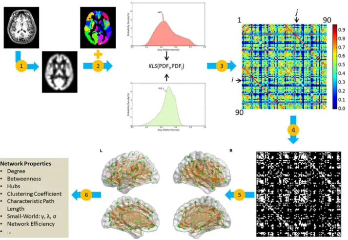
Fig 1. General workflow for the construction of an individual morphological network using gray matter measurements from MRI.(1) The estimation of gray matter volume as a morphological measure using a routine VBM procedure. (2) Brain parcellation with the AAL atlas and the estimation of
morphological distribution for each region. (3) Repeated quantification of the similarity between morphological distributions for pairs of regions and formation of the similarity matrix by filling in corresponding similarity values. (4) Extract the binarized matrix at a specific sparsity threshold. (5) Represent individual brain network as a graph. (6) Calculate the network metrics (e.g.,γ,λ, andσ). Note that, in this study steps 4–6 were repeated across a range of different sparsity thresholds, from 10% to 40% with an interval of 1%. HIP: Hippocampus; FFG: Fusiform gyrus; L: left; R: right; KLS: Kullback-Leibler divergence-based similarity; MRI: magnetic resonance imaging; VBM: voxel-divergence-based morphometry; AAL: automated anatomical labeling.
betweenness centrality. Global metrics included 1) small-world parameters, including the clus-tering coefficient (Cp), characteristic path length (Lp), and small-worldness (σ) and 2) network
efficiency involving global efficiency (Eg) and local efficiency (Eloc). These network metrics were calculated by using GRETNA toolbox [30].
Betweenness. Betweenness centrality (Bi) for nodeiis defined as the numbers of shortest
paths between any two nodes that pass through those nodes [31]. We measured normalized betweenness asbi=Bi/meanBet, wheremeanBetwas the average betweenness of all nodes in the
network. The betweenness values reflect the importance of the nodes within the entire network. Clustering Coefficient (Cp). The clustering coefficient (Cpi) of a node is equivalent to the
ratio of the node’s direct neighbors, which are also neighbors to each other [32]. The clustering coefficient (Cp) for the network is the average clustering coefficient for all nodes. Therefore, on average,Cpreflects the prevalence of clustered connectivity around individual nodes (i.e., func-tional segregation).
Characteristic Path Length (Lp). The characteristic path length (Lp) of a network is defined as the average shortest path length between all pairs of nodes [32] and the most commonly used measure of functional integration.
Small-World Properties. The small-world model was originally proposed by Watts and Strogatz (1998). Small-world networks have higher clustering coefficient relative to random networks and display similar characteristic path lengths to those of a random graph [32]. Small-worldness (σ) are defined as the division of the normalized clustering coefficient,Cp/
Cprand(i.e.,γ), and the normalized characteristic path length,Lp/Lprand(i.e.,λ) [33].Cprandand
Lprandare the network metrics for comparable random networks (averaged from 100
compara-ble random networks for each network) [34]. We generated these random networks using Maslov’s random rewiring algorithm [34], which preserves the same number of nodes, number of edges, and degree distribution as the real network.
Small-world networks are defined by a clustering coefficient (Cp), which is larger than
Cprand, or a normalized value forγlarger than 1 and characteristic path length (Lp) that is
approximately the same order as that of a comparable random graph or normalized value forλ
close to 1 [4]. In addition, the syncretic metric (σ) is higher than 1 in a small-world network.
Network Efficiency. Global efficiency (Eg) has been considered a superior measure of
inte-gration [35]. This network metric is defined as the average inverse shortest path length [35], which is related to the classical characteristic path length (Lp).
Further, the clustering coefficient can be regarded as a measure of the local efficiency of information delivery in the direct neighbors of each node. The local efficiency (Eloc) of the
net-work is estimated by averaging local efficiencies for all nodes in the graph.
Spatial Distribution of Hubs within the Networks. Important brain regions (i.e., hubs) often interact with many other regions. In this study, we applied normalized betweenness (bi) to
assess the importance of individual nodes, as it captures the node's influence on the informa-tion flow between other nodes in the network. To quantify similarity and uniqueness between individual networks, two metrics were defined based on the spatial distribution of nodal impor-tance; for the participantm, similarity to other participants was defined as average similarity with others, while uniqueness was defined as 1 minus maximal similarity with others. Specifi-cally, these metrics were defined as follows:
Similaritym¼
P
n2N; n6¼mcorrðBdm;BdnÞ
N 1
Uniquenessm¼1 max
whereNis the total number of participants andBdmis the betweenness of all nodes for
partici-pantm. The scores ranged from -1 to 1 and 0 to 2 for similarity and uniqueness, respectively. These scores were subsequently rescaled to the range [0, 1].
Finally, we identified hubs in the proposed network. Specifically, we first calculated the aver-age of the normalized betweenness centrality for each node across all participants and then defined hubs as nodes with an averaged betweenness value higher than one SD above the corre-sponding mean value across all nodes. To visualize the results, the BrainNet Viewer [22] was used.
Test-retest reliability
The scan-rescan dataset allowed us to quantify the test-retest reliability of the morphological networks for each participant. Intraclass correlation coefficients (ICCs) were calculated, as shown below [36]:
ICC¼ d 2
between d2
betweenþd
2
within
where the ICC is conceptualized as the ratio of between-subjects variance to total variance. The ICC is a quantity between 0 and 1, where 1 indicates perfect reliability (that is, the with-participant varianced2
withinis nearly 0). An ICC value above 0.75 is considered excellent. An
ICC value ranging from 0.59 to 0.75 is considered good, and results between 0.40 and 0.58 are considered fair [37,38]. In this study, the“irr”package (http://cran.r-project.org/web/ packages/irr/index.html) was used to estimate ICC values for each network metric assessed using individual networks over a wide range of sparsity thresholds.
Statistical analysis of individual differences in the morphological network
To demonstrate the usability of the morphological network proposed in this study, we illus-trated our approach with an exploratory study involving age-related changes in the brain net-work. In this analysis, we focused on the commonly used network metrics described above includingmeanBet,Lp,Lp,λ,γ,σ,Eg, andEloc. In the analysis with predefined sparsity (i.e.,
23%; seeThreshold Selection) used for display purposes in the study, a significant threshold of p<0.05 (FDR corrected for multiple comparisons) was applied. In addition, to ensure that the
findings were robust to data non-normality and to avoid the influence of possible outliers, Spearman’s rank-correlation coefficients were calculated for each correlation analysis. The same analyses were repeated over the range of sparsity threshold values from 10% to 40%. Given the exploratory nature of the analyses, uncorrected p values (p<0.05) were used.
Results
For the first time, we proposed a new network framework of the individual brain morphology to investigate the brain structure at the network level. The following analyses were conducted. First, we described the spatial pattern of the proposed morphological networks. Second, we examined the small-world properties of the networks. Then, the spatial distribution of hubs was investigated. Next, the robustness of our method was estimated. Finally, we conducted a correlation analysis to explore the age-related changes in the network metrics.
Description of the spatial pattern of the network
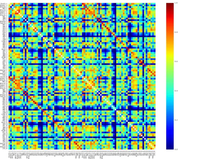
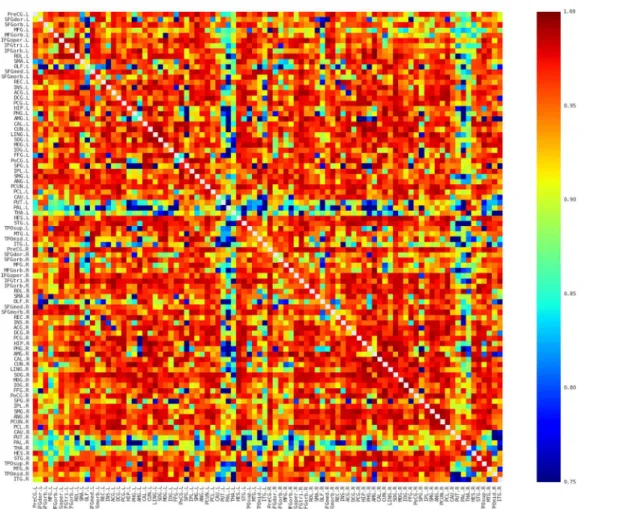
then averaged to reveal the similarity pattern of morphological distributions across partici-pants. Several interesting facts can be observed inFig 2. First, nearby regions showed similar connection pattern across the whole brain, such as STG, MTG, and ITG in the temporal regions, which is generally comparable with previous brain network studies (e.g., [39,40]). Sec-ond, consistent with previous brain network studies (e.g., [39–42]), the homotopic regions from the two hemispheres showed high inter-hemispheric connections. Third, some intra-hemispheric regions located in different lobes also showed high similarity of morphological distributions. For instance, the relative high similarity between the frontal (e.g., PreCG and IFG regions) and partial (e.g., IPL and SMG) regions might reflect the white matter connection among these regions (i.e., superior longitudinal fasciculus). In addition, connections with rela-tive high similarity showed relarela-tive low CV (top 5% connections: CV = 0.18; top 10%:
CV = 0.22; top 20%: CV = 0.28; top 30%: CV = 0.31;Fig 3), suggesting considerable consistency across participants.
Small-World properties of the individual networks
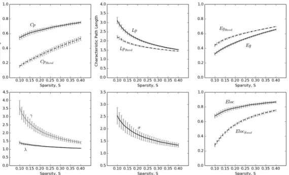
Next, we assessed the small-world properties of individual morphological networks. Initially, their clustering coefficient (Cp) and characteristic path length (Lp) were compared with those from the comparable randomized networks. As expected, the clustering coefficients (Cp) for
Fig 2. The averaged map of the connectivity matrices.Red and blue color indicates high and low similarity between regions, respectively. Main diagonal (i.e., self-connection) is indicated in white and excluded from following analyses. L, Left; R, Right.
the extracted networks displayed significantly higher values, relative to those of the randomized networks, over wide sparsity thresholds (Fig 4, upper left; paired t test, range of t values: min = 44.706; max = 72.949; all ps<8.502 × 10⁻³⁰). Similarly,γ(i.e.,Cp/Cprand) was larger than 1 (Fig 4, bottom left; range of averageγvalues: min = 1.416; max = 3.561), which satisfied the small-world network criterion. The characteristic path lengths (Lp) of the individual net-works were also higher relative to those of the randomized netnet-works (Fig 4, upper right; paired t-test, range of t values: min = 30.489; max = 61.904; all ps<8.502 × 10⁻³⁰). However, as shown in the bottom-left panel ofFig 4, the ratio ofλ(i.e.,Lp/Lprand) was close to 1 (range of averageλvalues: min = 1.062; max = 1.406), which also satisfied the small-world network crite-rion. Further, as expected, the small-worldness (σ)of these networks also displayed values
larger than 1 (Fig 4, bottom right; range of the averageσvalues: min = 1.333; max = 2.543),
supporting the small-world topology of the individual morphological networks extracted using our proposed method.
Previous morphological, anatomical, and functional network studies that reported network properties with similar network sizes within a predefined sparsity threshold (i.e., 23%, see
Materials and Methods) in healthy individuals are summarized inTable 1. Another study [43] on individual morphological networks based on Tijms et al. (2012) shows similar global (Eg:
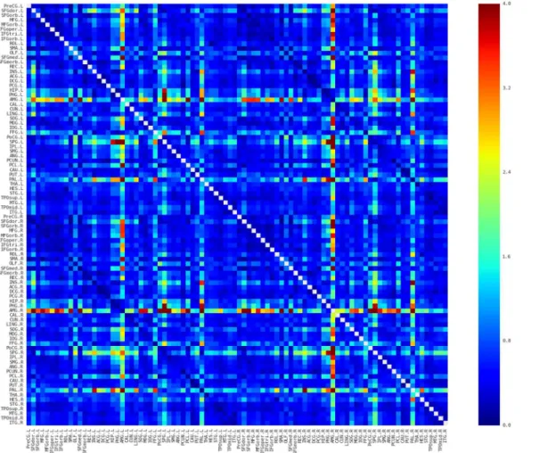
Fig 3. Coefficient of variation (CV) map of the connectivity matrices.Red and blue color indicates high and low dispersion of that connection across participants, respectively. Most of the connections possessed relative low CV and in particular the connections with relative high similarities showed low CV, suggesting relative high consistency across subjects. Main diagonal (i.e., self-connection) is indicated in white and excluded from following analyses. L, Left; R, Right.
~0.53) and local efficiency (Eloc: ~0.77) as ours (Eg: 0.52; Eloc: 0.80) (Fig 4), though informa-tion on small-world properties such asγandλis not available for comparison. The results indi-cated that the small-world properties in this study were comparable to those of previous studies.
Spatial distribution of hubs within the networks
In addition to the investigation of the small-world properties of the individual morphological networks, we also examined the spatial distribution of hubs (nodes with a normalized betweenness centrality higher than one SD above the mean for all nodes). Betweenness cen-trality is an important nodal metric that can be used to determine the relative importance of a node within the whole network and identify hubs in the complex networks, including the brain network (e.g., [18,28]).Fig 5Ashows the individual spatial distributions for 3 ran-domly selected participants, with larger spheres representing a higher betweenness value. The results visually showed that each individual exhibited a unique (though similar) spatial distribution. To give a quantitative description of the similarity and uniqueness of individual networks, we introduced two metrics respectively. Briefly, for one participant, the similarity to others is defined based on the average similarity with others, while the uniqueness is defined based on the value of 1 minus the maximal similarity with others. Results showed that individual networks possessed remarkable similarity (around 0.60;Fig 5B, left) as well as considerable uniqueness (around 0.3;Fig 5B, right) across different sparsity thresholds. The considerable uniqueness of individual networks may reflect the individual variability of brain anatomy [50,51], while the remarkable similarity may reflect the consistent organization of human brain network (e.g., [16]).
Next, the hubs in the proposed network were identified (seeMaterials and Methods). Results showed that 14 hubs, including 10 heteromodal or unimodal associative regions, 2 regions of the primary motor cortex, and 2 paralimbic regions, were identified (Fig 5C;
Fig 4. Small-world properties of the morphometric networks as a function of network sparsity thresholds.The error bar indicates the standard deviation.
Table 2). All of these regions have been reported as hubs at least once in previous study (Table 2).
Moreover, we revealed that the spatial distributions of hubs showed considerably more sim-ilarity (mean = 0.83, SD = 0.04) relative to its uniqueness (mean = 0.02, SD = 0.02) across dif-ferent thresholds, suggesting that the observed spatial distribution of hubs is unlikely accounted for by any specific threshold.
Test-retest reliability of the network metrics
To assess the robustness of our method, we estimated the ICC values for both the raw connec-tions and each network metric with the test-retest MRI data (scanned twice). As shown in
Fig 6, the connection values showed excellent reliability (mean ICC = 0.933, SD = 0.075) at the connection level; more than 97% of the edges possessed excellent reliability (i.e., ICC>0.75),
suggesting the high reliability of the proposed network.
As expected, the network metrics also showed considerable reliability (Fig 7). Under the predefined sparsity threshold value (23%), all commonly used network metrics displayed fair to excellent reliability (Lp: ICC = 0.657, p = 0.00044;Cp: ICC = 0.746, p = 2.09 × 10⁻⁵;λ: ICC = 0.428, p = 0.027;γ: ICC = 0.832, p = 7.24 × 10⁻⁷;σ: ICC = 0.871, p = 5.77 × 10⁻⁸;Eloc:
ICC = 0.781, p = 7.34 × 10⁻⁶;Eg: ICC = 0.665, p = 0.00038;meanBet: ICC = 0.743,
p = 2.47 × 10⁻⁵). Reliability analysis of these network metrics, assessed over a wide range of sparsity threshold values, indicated that the clustering coefficient (Cp) was highly stable (mean ICC = 0.740) for most of the sparsity values with which to threshold the morphological net-work, as were characteristic path length (Lp, mean ICC = 0.716),γ(mean ICC = 0.812),σ
(mean ICC = 0.848), and global efficiency (Eg, mean ICC = 0.744). In addition,λ(mean ICC = 0.637), local efficiency (Eloc, mean ICC = 0.683), and betweenness centrality (meanBet, mean ICC = 0.717) were reproducible (seeTable 3). Taken together, these results indicate the robustness of the proposed method for constructing individual morphological networks from gray matter MRI scans.
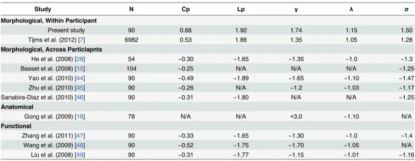
Table 1. Small-world properties in the present study, and for comparison, values from previous morphometric, anatomical, and functional studies.
Study N Cp Lp γ λ σ
Morphological, Within Participant
Present study 90 0.66 1.92 1.74 1.15 1.50
Tijms et al. (2012) [7] 6982 0.53 1.86 1.35 1.05 1.28
Morphological, Across Particiapnts
He et al. (2008) [28] 54 ~0.30 ~1.65 ~1.35 ~1.0 ~1.3
Basset et al. (2008) [15] 104 ~0.25 N/A N/A N/A ~1.25
Yao et al. (2010) [44] 90 ~0.49 ~1.89 ~1.65 ~1.10 ~1.47
Zhu et al. (2010) [45] 90 ~0.26 N/A ~1.2 ~1.03 ~1.17
Sanabira-Diaz et al. (2010) [46] 90 ~0.31 ~1.80 N/A N/A ~1.25
Anatomical
Gong et al. (2009) [18] 78 N/A N/A <3.0 ~1.10 N/A
Functional
Zhang et al. (2011) [47] 90 ~0.33 ~1.65 ~1.30 ~1.0 ~1.4
Wang et al. (2009) [48] 90 ~0.52 ~1.75 ~1.70 ~1.05 N/A
Liu et al. (2008) [49] 90 ~0.31 ~1.77 ~1.15 ~1.01 ~1.16
Note that the small-world properties from previous studies are all from healthy individuals. N: number of nodes used; N/A: Not Available.
Applying the morphological network metrics to examine normal aging
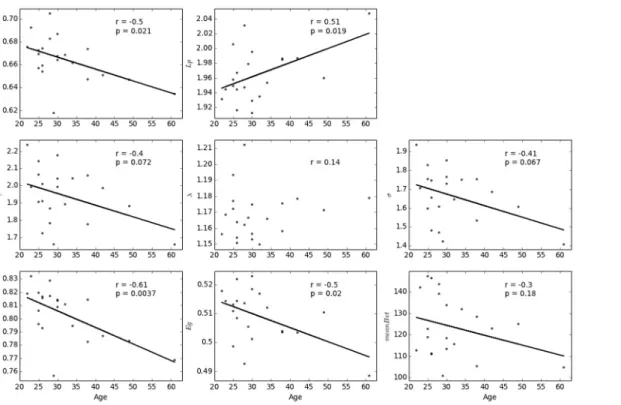
To demonstrate the usability of our method, we calculated the correlation between participant age and each of these network metrics assessed from individual networks. First, we conducted the analysis with a predefined threshold (i.e., 23%). As shown inFig 8, significant age-related
Fig 5. Spatial distribution of hubs within the morphometric network.(A) Three examples of the spatial distributions for betweenness. (B) The similarity (left) and uniqueness (right) of individual spatial distributions. (C) Hubs identified in this study. L: left; R: right. PreCG: precentral gyrus; IFGoper: inferior frontal gyrus opercularis; IFGtri: inferior frontal gyrus triangularis; SMA: supplementary motor area; SMG: supramarginal gyrus; PCUN: precuneus; TPOsup: superior temporal gyrus of temporal pole; MTG: middle temporal gyrus; ITG: inferior temporal gyrus.
changes (p<0.05, FDR corrected for multiple comparisons) were observed in the clustering coefficient (Cp, r = -0.50, p = 0.021; Spearman rho = -0.50, p = 0.021) and local efficiency (Eloc, r = -0.61, p = 0.0036; Spearman rho = -0.61, p = 0.0032). In addition, the effects of age on char-acteristic path length (Lp, r = 0.51, p = 0.019) and global efficiency (Eg, r = -0.50, p = 0.020) dis-played notable trends but failed to reach statistical significance using Spearman’s rank-correlation (Lp: Spearman rho = 0.35, p = 0.12;Eg: Spearman rho = -0.35, p = 0.12). No signifi-cant age-related changes were observed inγ(r = -0.40, p = 0.072; Spearman rho = -0.34, p = 0.13),σ(r = -0.408, p = 0.067; Spearman rho = -0.30, p = 0.19), betweenness centrality
(meanBet, r = -0.30, p = 0.18; Spearman rho = -0.22, p = 0.32), orλ(r = 0.14, p = 0.54; Spear-man rho = 0.10, p = 0.64). Even with the most conservative correction approach for multiple comparisons (i.e., Bonferroni correction), the effects of age on the local efficient (Eloc) remained (p = 0.0036<0.05/8). The significant change inElocof individual morphological
network indicates the age-related defect in local information delivery in the complex brain net-works, which is in line with previous findings on white matter networks [19].
Results of analysis with a sparsity threshold value range of 10% to 40% are shown inFig 9. Sig-nificant age-related changes (p<0.05, uncorrected) in clustering coefficient (Cp) and local
effi-ciency (Eloc) were observed for most of the sparsity values. In addition, the age-related changes in
σandγwere significant at higher sparsity values (S33%). Characteristic path length (Lp),
global efficiency (Eg), and normalized betweenness centrality (meanBet) also displayed significant age-related associations with some of the sparsity threshold values (Lp: 20%S24%;Eg: 20%
S24%;meanBet: 11%S20%). No significant associations were found observed withλ
for any of the sparsity threshold values (max correlation value: r = 0.42, p = 0.057 with S = 33%). In summary, our findings indicate the potential of the new approach to study the morpho-logical networks of individual participants.
Discussion
We proposed a novel network framework for individual brain morphology. The method was built on our recent work estimating interregional relation based on morphological
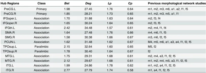
Table 2. Cortical regions identified as hubs in the morphometric network and their properties.
Hub Regions Class Bet Deg Lp Cp Previous morphological network studies
PreCG.L Primary 1.98 27.45 1.76 0.64 m1, m2, m3, m6, a1, a2, f1, f5
PreCG.R Primary 1.85 28.21 1.73 0.65 m1, m2, m3, m5, a1, f1
IFGoper.L Association 1.70 31.88 1.63 0.64 m2, f3, f4
IFGoper.R Association 1.65 30.24 1.64 0.65 m2, f3, f5
IFGtri.L Association 2.42 34.48 1.57 0.61 m2, m4, f1, f4
SMA.R Association 1.64 27.48 1.76 0.66 m4, m6, f1, f5
SMG.R Association 1.58 30.38 1.66 0.67 m3, m6, f2, f5
PCUN.L Association 1.62 31.48 1.62 0.67 M4, m5, m6, a1, a3, a4, f1, f2, f5
TPOsup.L Paralimbic 2.15 32.64 1.60 0.65 M5, f2
TPOsup.R Paralimbic 1.78 30.40 1.64 0.67 f2
MTG.L Association 1.75 29.31 1.68 0.61 m2, m4, a3, f1, f2, f5
MTG.R Association 2.12 29.67 1.68 0.61 m1, m2, m4, m5, a3, f1, f2, f5
ITG.L Association 1.99 24.86 1.78 0.62 m1, m2, a4, f1, f2, f5
ITG.R Association 2.77 27.79 1.74 0.58 m1, a4, f1, f2, f5
We compared the results with previous morphological network studies: m1 = [15], m2 = [52], m3 = [7], m4 = [27], m5 = [44] and m6 = [45]; anatomical network studies: a1 = [18], a2 = [19], a3 = [53], and a4 = [25]; and functional network studies: f1 = [54], f2 = [50], f3 = [55], f4 = [56], and f5 = [57].
distributions, by extending it into the research field of complex brain networks. The proposed method was able to construct and investigate brain networks for each participant, using MRI scans. With the use of graph-theoretical approaches, we found that all networks possessed small-world properties (i.e., they had a higher clustering coefficient relative to random net-works and a similar minimum path length to that of comparable randomized netnet-works). The values of the clustering and small-world coefficients were compatible with previous structural and functional network results (seeTable 1). The morphological network also displayed hubs, all of which have been reported in previous network studies (seeTable 2). In addition, the net-work metrics were reproducible, supporting the robustness of the method (seeTable 3). Finally, the correlation analysis indicated that most of the network metrics reflected normal aging. Taken together, these results suggest that the new network could provide a concise description of the organization of an individual brain. Further, our approach provides a novel perspective on understanding of brain morphology and would further facilitate the emerging field of human connectomics.
Inter-regional similarity of morphological distribution
It is noteworthy that, in this study, the inter-regional connection was quantified with similarity in distributions of local brain morphology. The inter-regional similarity metric has just been
Fig 6. The Intraclass Correlation Coefficient (ICC) map of the connectivity matrices.More than 97% of the edges showed excellent reliability (i.e., ICC>0.75).
proposed recently and suggested to be informative for the study of brain morphology [8] How-ever, it is almost entirely unknown whether this metric would provide benefits for mapping human whole-brain networks. The present study is, to our knowledge, the first to construct brain networks with regional morphological distribution information. In previous morphologi-cal network studies, networks have usually been constructed using correlations between aver-age cortical areas, with respect to thickness or volume, across participants [15,52,58]. Another approach for mapping vertex-wise anatomical correlations has also been proposed [59].
Fig 7. Test-retest reliability with intraclass correlation coefficient (ICC) for each of the network metrics as a function of network sparsity thresholds.The smallest ICC at various sparsity thresholds for each network metric is listed for the following:Cp: min ICC = 0.605, p = 0.0018;Lp: min ICC = 0.518, p = 0.0060;γ: min ICC = 0.636, p = 0.0020;λ: min ICC = 0.391, p = 0.035;σ: min ICC = 0.611, p = 0.00092;Eloc: min ICC = 0.377, p = 0.047;Eg: min ICC = 0.611, p = 0.0014;meanBet: min ICC = 0.485, p = 0.012.
doi:10.1371/journal.pone.0141840.g007
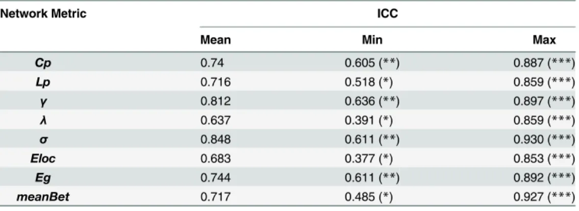
Table 3. A summary of test-retest reliability with intraclass correlation coefficient (ICC) for each of the network metrics.
Network Metric ICC
Mean Min Max
Cp 0.74 0.605 (**) 0.887 (***)
Lp 0.716 0.518 (*) 0.859 (***)
γ 0.812 0.636 (**) 0.897 (***)
λ 0.637 0.391 (*) 0.859 (***)
σ 0.848 0.611 (**) 0.930 (***)
Eloc 0.683 0.377 (*) 0.853 (***)
Eg 0.744 0.611 (**) 0.892 (***)
meanBet 0.717 0.485 (*) 0.927 (***)
*: p<0.05; **: p<0.005; ***: p<0.0001.
Fig 8. Age-related changes in each of the network metrics at a predefined sparsity threshold (i.e., 23%).
doi:10.1371/journal.pone.0141840.g008
Fig 9. Age-related changes in each of the network metrics over the range of sparsity thresholds.The star markers (correlations falling outside the shaded area) indicate significant correlations (p<0.05).
However, such correlation-based approaches could only construct one network per group and required the analysis of networks at a large-group level.
In contrast, our method allows construction of individual brain networks using MRI images. More importantly, given that MRI images are widely available and convenient to collect, the pro-posed method could provide a novel perspective on the understanding of individual variability and clinical conditions. For example, this method could provide a more comprehensive means of automatically identifying brain abnormalities in a single participant’s brain. To construct indi-vidual networks based on MRI images, interesting methods have been used in particular con-texts, which were based on average measures for different regions [60,61] or even data from other participants [61]. Recently, Tijms et al. (2012) proposed an alternative method with which to extract individual networks using MRI scans of GM. Briefly, the method begins by defining approximately 6,982 nodes that correspond to 3 × 3 × 3 voxel cubes. The similarity between the nodes in the network is determined using correlation coefficients between two separate sets of 27 voxels from two cubes. This approach provides a new perspective on the examination of individ-ual MRI data. However, in this approach, the rigid extraction of the small cubes may not allow optimal correspondence to functionally and anatomically homogeneous regions or convolutions of the brain [7], and under this framework, one has no choice but to define nodes as completely regular small regions with the same shape and size. Moreover, this approach can result in the problem of different network sizes for individual networks. This problem can be solved with a follow-up normalization strategy [43]. However, the cube size and rotation operation used in both studies are somehow arbitrary and does not take the remarkable variability in the shapes and sizes of regions into account. The present study proposed a new network framework based on regional morphological distribution information, which would provide a novel perspective for understanding individual differences and even clinical abnormality.
In addition, an interregional relationship was defined based on local brain morphology. The physiological meaning underlying the new measure is complex and not completely understood [8]. One possible source of the morphological connections proposed here is the axon tension the-ory [62], which predicts that connected areas are pulled by a mechanical force, becoming either thinner or thicker. This is similar to the population-based morphological relationship found in previous studies [15,52]. An alternative possibility is that regions with similar morphological dis-tributions could have reflected developmental coordination or synchronized maturation between areas, which may be related to axonal connections forming and reforming over the course of early development [59,63]. Similarly, inter-regional relevance may also reflect common experi-ence-related plasticity [64,65]. Taken collectively, one could therefore speculate that individual morphological interregional relationships provide approximate reflection of true anatomical connections between neuronal elements. In addition, morphologically related regions may also share similar distributions of major cell classes (such as neurons, oligodendrocytes, and astro-cytes) and gene expression [66]. Note that the abovementioned biological underpinnings are speculative, and future studies on cell morphology or molecular genetics are needed. Neverthe-less, the novel method provides a reliable and meaningful description of the structure of individ-ual brains. In addition, since different morphological metrics, such as GM volume, thickness, and area, measure different aspects of GM structure and thus can provide complementary infor-mation about local GM, future work is needed to extend our framework to accommodate multi-ple morphological features to measure the morphological similarity between regions.
Spatial distribution of hubs
[67]. With the present method, we found consistent spatial distribution. As expected, the hubs identified (Fig 3C;Table 2) in the morphological network were also predominately involved in the recently evolved heteromodal (e.g., the PCUN [precuneus], MTG [middle temporal gyrus], and IFGtri [inferior frontal gyrus triangularis]) or unimodal (e.g., the SMA [supplementary motor area] and ITG [inferior temporal gyrus]) association cortex [67]. As shown inTable 2, all hubs involved in this study have been reported as hub regions in several previous human brain network studies. For example, the PCUN and MTG have also consistently been identified as hubs in previous morphological (e.g., [27,44]), anatomical (e.g., [53]), and functional (e.g., [54,68]) network studies.
Of note, although there was overlap between the sets of hubs reported in these studies, which indicates a degree of topological isomorphism between different modal networks, no two studies have reported identical sets of hub regions. This discrepancy may have been caused by methodological differences, such as brain imaging parameters, connection and node defini-tion, and the populations involved. Further systematic studies exploring hubs in brain net-works from different modalities, with the same criteria of network analysis and in a similar population, would provide a deeper understanding of hubs in the human brain.
In addition, at an individual level, we found that participants showed unique (though simi-lar) spatial distribution of betweenness values (Fig 3A and 3B). The considerable uniqueness observed may reflect the individual variability of brain anatomy [50,51]. However, thus far, few studies have examined variability in hub distribution with anatomical, morphological, or functional brain networks. In response to this issue, we introduced two metrics to quantify the uniqueness and similarity of individual networks. We hope that further investigations into the source and outcome of this variability will benefit from these metrics.
Furthermore, as hubs have been identified as core regions with multimodal or integrative functions, their damage can affect the stability and efficiency of the network significantly [54,
69]. Studies conducted to determine whether patients with neurological diseases, particularly those with abnormality or deficit in the association cortex, have altered network attributes (e.g., small-world properties and modularity) in individual morphological networks are urgently required.
Age effect on the network metrics
et al. (2012). Further, considering the relatively small sample size and complicated (and non-linear) fashion in which network properties were computed, further systematic studies with larger cohorts and more flexible statistical models are required. Nonetheless, the present find-ings demonstrated potential for use in revealing presumed whole-brain network individual dif-ferences in healthy populations and abnormalities in participants with neurological and psychiatric disorders, as have been found in anatomical [71–73], functional [74–76], and popu-lation-based morphological networks [15,26,44].
Methodological issues and future research
The present study was subject to some methodological issues that should be addressed. First, we defined connections in the networks based on morphological distributions. There-fore, accurately estimation of such distributions is of critical importance. On one hand, there should be a sufficiently large sample from such a distribution. In the present study, the AAL atlas was used to obtain macroscopic parcellation of the brain, as in previous studies (e.g., [18]). For each region, there were sufficiently large observations (larger than 120), which ensured accurate estimation of regional morphological distributions. In addition, with increas-ing resolution, morphological networks could also be based on finer parcellation of the brain. On the other hand, in the present study, Gaussian KDE [20] was used to estimate morphologi-cal distributions. Although the present method was initially validated [8] and appears to pro-duce good approximations, it would be interesting to examine how different estimation methods influence individual morphological networks.
Second, in the present study, we binarized each network repeatedly over a wide range of sparsity thresholds, as in previous morphological network studies [7,26,27]. This was per-formed in consideration of the absence of a definitive method for selecting a single threshold. Given continuous weights contain more information [23,24], it is also possible to characterize the brain as weighted networks. However, the weighted models may lead to complicated statis-tical descriptions in the graph theorestatis-tical analyses [52,75,77], so we confined our analyses to a simple binary network analysis. It is worthy of applying graph theoretical methods to the weighted networks to investigate the topological properties of the individual morphological networks in future studies.
Third, the network analysis in the present study was based on the AAL template. As previ-ous network studies with either resting-state fMRI or diffusion MRI have suggested that the measure of similarities likely depended on the choice of brain templates to some extent [48,
78], which is an inevitable limitation of any method on large-scale brain network. Future stud-ies are needed to quantify whether and how different templates (e.g., the Harvard-Oxford atlas) affects network properties (e.g., small-world properties) of individual morphological net-work. In addition, it is a potential topic to construct and investigate the individual morphologi-cal networks with features, such as thickness, area and curvature, and brain parcellation derived in the native space.
Fourth, the test-retest reliability was performed based on the datasets collected in the same day to ruling out unwanted effects of training or experience. However, this was short-term reli-ability, and further studies are needed to examine long-term reliability for this method [79].
as in-scanner head motion [81–83]. In this case, researchers could explore the different net-work properties during the performance of different tasks. Similarly, these netnet-works may also reflect individual differences in task performance. As another example, in constructing a brain network using the only ultrahigh-resolution brain model, BigBrain [84], the similarity of regional distribution in microscopic data may result in a concise and meaningful measure of connections at an almost cellular level. In all, it would be interesting to explore more detailed patterns using these local features from the perspective of complex networks.
Conclusions
Complex network analysis has emerged as an important tool in the characterization of anatom-ical, functional, and morphological brain connectivity. We proposed a new framework for con-structing individual morphological networks using MRI data with our newly-developed interregional relation metric based on regional morphological distributions. Results showed that the morphological networks possessed prominent small-world properties and spatial dis-tribution of pivotal regions, mainly the association cortex regions. In addition, the network metrics displayed excellent reliability, which supports the robustness of the method. Our find-ings are largely compatible with previous human brain network studies. In summary, our method may provide a novel insight into the cerebral organization that underlie interindividual variability in behavioral and cognitive performance and clinical conditions. We hope that the brain mapping community will benefit from and contribute to this novel method.
Acknowledgments
We thank Yi Pu for helpful discussions and critical reading of the manuscript. We give specific thanks to Bennett Landman for data sharing.
Author Contributions
Conceived and designed the experiments: XK ZL ZZ LH XW. Performed the experiments: XK ZL ZY GZ ZZ. Analyzed the data: XK. Contributed reagents/materials/analysis tools: XK. Wrote the paper: XK ZZ JL.
References
1. Ashburner J, Friston KJ. Voxel-based morphometry—the methods. Neuroimage. 2000; 11(6 Pt 1):805–
21. PMID:10860804
2. Kanai R, Rees G. The structural basis of inter-individual differences in human behaviour and cognition. Nat Rev Neurosci. 2011; 12(4):231–42. doi:10.1038/nrn3000PMID:21407245
3. Sporns O, Chialvo DR, Kaiser M, Hilgetag CC. Organization, development and function of complex brain networks. Trends Cogn Sci. 2004; 8(9):418–25. PMID:15350243
4. Bullmore E, Sporns O. Complex brain networks: graph theoretical analysis of structural and functional systems. Nat Rev Neurosci. 2009; 10(3):186–98. doi:10.1038/nrn2575PMID:19190637
5. He Y, Wang L, Zang Y, Tian L, Zhang X, Li K, et al. Regional coherence changes in the early stages of Alzheimer's disease: a combined structural and resting-state functional MRI study. Neuroimage. 2007; 35(2):488–500. PMID:17254803
6. Wen W, He Y, Sachdev P. Structural brain networks and neuropsychiatric disorders. Curr Opin Psychi-atry. 2011; 24(3):219–25. PMID:21430538
7. Tijms BM, Series P, Willshaw DJ, Lawrie SM. Similarity-based extraction of individual networks from gray matter MRI scans. Cereb Cortex. 2012; 22(7):1530–41. doi:10.1093/cercor/bhr221PMID: 21878484
9. Savadjiev P, Rathi Y, Bouix S, Smith AR, Schultz RT, Verma R, et al. Fusion of white and gray matter geometry: a framework for investigating brain development. Med Image Anal. 2014; 18(8):1349–60. doi:10.1016/j.media.2014.06.013PMID:25066750
10. Landman BA, Huang AJ, Gifford A, Vikram DS, Lim IA, Farrell JA, et al. Multi-parametric neuroimaging reproducibility: a 3-T resource study. Neuroimage. 2011; 54(4):2854–66. doi:10.1016/j.neuroimage. 2010.11.047PMID:21094686
11. Mugler JP 3rd, Brookeman JR. Three-dimensional magnetization-prepared rapid gradient-echo imag-ing (3D MP RAGE). Magn Reson Med. 1990; 15(1):152–7. PMID:2374495
12. Mechelli A, Price CJ, Friston KJ, Ashburner J. Voxel-Based Morphometry of the Human Brain: Methods and Applications. Curr Med Imaging Rev. 2005; 1:105–13.
13. Ashburner J. A fast diffeomorphic image registration algorithm. Neuroimage. 2007; 38(1):95–113. PMID:17761438
14. Good CD, Johnsrude IS, Ashburner J, Henson RN, Friston KJ, Frackowiak RS. A voxel-based morpho-metric study of ageing in 465 normal adult human brains. Neuroimage. 2001; 14(1 Pt 1):21–36. PMID: 11525331
15. Bassett DS, Bullmore E, Verchinski BA, Mattay VS, Weinberger DR, Meyer-Lindenberg A. Hierarchical organization of human cortical networks in health and schizophrenia. J Neurosci. 2008; 28(37):9239–
48. doi:10.1523/JNEUROSCI.1929-08.2008PMID:18784304
16. Sporns O, Tononi G, Kotter R. The human connectome: A structural description of the human brain. PLoS Comput Biol. 2005; 1(4):e42. PMID:16201007
17. Tzourio-Mazoyer N, Landeau B, Papathanassiou D, Crivello F, Etard O, Delcroix N, et al. Automated anatomical labeling of activations in SPM using a macroscopic anatomical parcellation of the MNI MRI single-subject brain. Neuroimage. 2002; 15(1):273–89. PMID:11771995
18. Gong G, He Y, Concha L, Lebel C, Gross DW, Evans AC, et al. Mapping anatomical connectivity pat-terns of human cerebral cortex using in vivo diffusion tensor imaging tractography. Cereb Cortex. 2009; 19(3):524–36. doi:10.1093/cercor/bhn102PMID:18567609
19. Gong G, Rosa-Neto P, Carbonell F, Chen ZJ, He Y, Evans AC. Age- and gender-related differences in the cortical anatomical network. J Neurosci. 2009; 29(50):15684–93. doi: 10.1523/JNEUROSCI.2308-09.2009PMID:20016083
20. Bowman AW, Azzalini A, editors. Applied Smoothing Techniques for Data Analysis. New York: Oxford University Press; 1997.
21. Scott DW, editor. Multivariate Density Estimation: Theory, Practice, and Visualization. New York: John Wiley & Sons; 1992.
22. Xia M, Wang J, He Y. BrainNet Viewer: a network visualization tool for human brain connectomics. PLoS One. 2013; 8(7):e68910. doi:10.1371/journal.pone.0068910PMID:23861951
23. Barrat A, Barthelemy M, Pastor-Satorras R, Vespignani A. The architecture of complex weighted net-works. Proc Natl Acad Sci U S A. 2004; 101(11):3747–52. PMID:15007165
24. Jiang T, He Y, Zang Y, Weng X. Modulation of functional connectivity during the resting state and the motor task. Hum Brain Mapp. 2004; 22(1):63–71. PMID:15083527
25. van den Heuvel MP, Mandl RC, Stam CJ, Kahn RS, Hulshoff Pol HE. Aberrant frontal and temporal complex network structure in schizophrenia: a graph theoretical analysis. J Neurosci. 2010; 30 (47):15915–26. doi:10.1523/JNEUROSCI.2874-10.2010PMID:21106830
26. He Y, Dagher A, Chen Z, Charil A, Zijdenbos A, Worsley K, et al. Impaired small-world efficiency in structural cortical networks in multiple sclerosis associated with white matter lesion load. Brain. 2009; 132(Pt 12):3366–79. doi:10.1093/brain/awp089PMID:19439423
27. Wu K, Taki Y, Sato K, Kinomura S, Goto R, Okada K, et al. Age-related changes in topological organi-zation of structural brain networks in healthy individuals. Hum Brain Mapp. 2012; 33(3):552–68. doi:10. 1002/hbm.21232PMID:21391279
28. He Y, Chen Z, Evans A. Structural insights into aberrant topological patterns of large-scale cortical net-works in Alzheimer's disease. J Neurosci. 2008; 28(18):4756–66. doi:10.1523/JNEUROSCI.0141-08. 2008PMID:18448652
29. Bassett DS, Bullmore E. Small-world brain networks. Neuroscientist. 2006; 12(6):512–23. PMID: 17079517
30. Wang J, Wang X, Xia M, Liao X, Evans A, He Y. GRETNA: a graph theoretical network analysis toolbox for imaging connectomics. Front Hum Neurosci. 2015; 9:386. doi:10.3389/fnhum.2015.00386 PMID:26175682
32. Watts DJ, Strogatz SH. Collective dynamics of 'small-world' networks. Nature. 1998; 393(6684):440–2. PMID:9623998
33. Humphries MD, Gurney K. Network 'small-world-ness': a quantitative method for determining canonical network equivalence. PLoS One. 2008; 3(4):e0002051. doi:10.1371/journal.pone.0002051PMID: 18446219
34. Maslov S, Sneppen K. Specificity and stability in topology of protein networks. Science. 2002; 296 (5569):910–3. PMID:11988575
35. Latora V, Marchiori M. Efficient behavior of small-world networks. Phys Rev Lett. 2001; 87(19):198701. PMID:11690461
36. Shrout PE, Fleiss JL. Intraclass correlations: uses in assessing rater reliability. Psychol Bull. 1979; 86 (2):420–8. PMID:18839484
37. Bennett CM, Miller MB. How reliable are the results from functional magnetic resonance imaging? Ann N Y Acad Sci. 2010; 1191:133–55. doi:10.1111/j.1749-6632.2010.05446.xPMID:20392279
38. Cicchetti D, Sparrow S. Developing criteria for establishing interrater reliability of specific items: Appli-cations to assessment of adaptive behavior. American Journal of Mental Deficiency. 1981; 86(2):127–
37. PMID:7315877
39. Bernhardt BC, Chen Z, He Y, Evans AC, Bernasconi N. Graph-theoretical analysis reveals disrupted small-world organization of cortical thickness correlation networks in temporal lobe epilepsy. Cereb Cortex. 2011; 21(9):2147–57. doi:10.1093/cercor/bhq291PMID:21330467
40. He Y, Wang J, Wang L, Chen ZJ, Yan C, Yang H, et al. Uncovering intrinsic modular organization of spontaneous brain activity in humans. PLoS One. 2009; 4(4):e5226. doi:10.1371/journal.pone. 0005226PMID:19381298
41. Sanz-Arigita EJ, Schoonheim MM, Damoiseaux JS, Rombouts SA, Maris E, Barkhof F, et al. Loss of 'small-world' networks in Alzheimer's disease: graph analysis of FMRI resting-state functional connec-tivity. PLoS One. 2010; 5(11):e13788. doi:10.1371/journal.pone.0013788PMID:21072180
42. Khundrakpam BS, Reid A, Brauer J, Carbonell F, Lewis J, Ameis S, et al. Developmental changes in organization of structural brain networks. Cereb Cortex. 2013; 23(9):2072–85. doi:10.1093/cercor/ bhs187PMID:22784607
43. Batalle D, Munoz-Moreno E, Figueras F, Bargallo N, Eixarch E, Gratacos E. Normalization of similarity-based individual brain networks from gray matter MRI and its association with neurodevelopment in infants with intrauterine growth restriction. Neuroimage. 2013; 83:901–11. doi:10.1016/j.neuroimage. 2013.07.045PMID:23886985
44. Yao Z, Zhang Y, Lin L, Zhou Y, Xu C, Jiang T. Abnormal cortical networks in mild cognitive impairment and Alzheimer's disease. PLoS Comput Biol. 2010; 6(11):e1001006. doi:10.1371/journal.pcbi. 1001006PMID:21124954
45. Zhu W, Wen W, He Y, Xia A, Anstey KJ, Sachdev P. Changing topological patterns in normal aging using large-scale structural networks. Neurobiol Aging. 2012; 33(5):899–913. doi:10.1016/j. neurobiolaging.2010.06.022PMID:20724031
46. Sanabria-Diaz G, Melie-Garcia L, Iturria-Medina Y, Aleman-Gomez Y, Hernandez-Gonzalez G, Val-des-Urrutia L, et al. Surface area and cortical thickness descriptors reveal different attributes of the structural human brain networks. Neuroimage. 2010; 50(4):1497–510. doi:10.1016/j.neuroimage. 2010.01.028PMID:20083210
47. Zhang J, Wang J, Wu Q, Kuang W, Huang X, He Y, et al. Disrupted brain connectivity networks in drug-naive, first-episode major depressive disorder. Biol Psychiatry. 2011; 70(4):334–42. doi:10.1016/j. biopsych.2011.05.018PMID:21791259
48. Wang J, Wang L, Zang Y, Yang H, Tang H, Gong Q, et al. Parcellation-dependent small-world brain functional networks: a resting-state fMRI study. Hum Brain Mapp. 2009; 30(5):1511–23. doi:10.1002/ hbm.20623PMID:18649353
49. Liu Y, Liang M, Zhou Y, He Y, Hao Y, Song M, et al. Disrupted small-world networks in schizophrenia. Brain. 2008; 131(Pt 4):945–61. doi:10.1093/brain/awn018PMID:18299296
50. Amunts K, Schleicher A, Burgel U, Mohlberg H, Uylings HB, Zilles K. Broca's region revisited: cytoarchi-tecture and intersubject variability. J Comp Neurol. 1999; 412(2):319–41. PMID:10441759
51. Westbury CF, Zatorre RJ, Evans AC. Quantifying variability in the planum temporale: a probability map. Cereb Cortex. 1999; 9(4):392–405. PMID:10426418
52. He Y, Chen ZJ, Evans AC. Small-world anatomical networks in the human brain revealed by cortical thickness from MRI. Cereb Cortex. 2007; 17(10):2407–19. PMID:17204824
54. Achard S, Salvador R, Whitcher B, Suckling J, Bullmore E. A resilient, low-frequency, small-world human brain functional network with highly connected association cortical hubs. J Neurosci. 2006; 26 (1):63–72. PMID:16399673
55. Jin SH, Jeong W, Seol J, Kwon J, Chung CK. Functional cortical hubs in the eyes-closed resting human brain from an electrophysiological perspective using magnetoencephalography. PLoS One. 2013; 8(7): e68192. doi:10.1371/journal.pone.0068192PMID:23874535
56. Meunier D, Achard S, Morcom A, Bullmore E. Age-related changes in modular organization of human brain functional networks. Neuroimage. 2009; 44(3):715–23. doi:10.1016/j.neuroimage.2008.09.062 PMID:19027073
57. Shehzad Z, Kelly AM, Reiss PT, Gee DG, Gotimer K, Uddin LQ, et al. The resting brain: unconstrained yet reliable. Cereb Cortex. 2009; 19(10):2209–29. doi:10.1093/cercor/bhn256PMID:19221144
58. Chen ZJ, He Y, Rosa-Neto P, Germann J, Evans AC. Revealing modular architecture of human brain structural networks by using cortical thickness from MRI. Cereb Cortex. 2008; 18(10):2374–81. doi:10. 1093/cercor/bhn003PMID:18267952
59. Lerch JP, Worsley K, Shaw WP, Greenstein DK, Lenroot RK, Giedd J, et al. Mapping anatomical corre-lations across cerebral cortex (MACACC) using cortical thickness from MRI. Neuroimage. 2006; 31 (3):993–1003. PMID:16624590
60. Dai D, He H, Vogelstein JT, Hou Z. Accurate prediction of AD patients using cortical thickness net-works. Machine Vision and Applications. 2013; 24(7):1445–57.
61. Raj A, Mueller SG, Young K, Laxer KD, Weiner M. Network-level analysis of cortical thickness of the epileptic brain. Neuroimage. 2010; 52(4):1302–13. doi:10.1016/j.neuroimage.2010.05.045PMID: 20553893
62. Van Essen DC. A tension-based theory of morphogenesis and compact wiring in the central nervous system. Nature. 1997; 385(6614):313–8. PMID:9002514
63. Alexander-Bloch A, Raznahan A, Bullmore E, Giedd J. The convergence of maturational change and structural covariance in human cortical networks. J Neurosci. 2013; 33(7):2889–99. doi:10.1523/ JNEUROSCI.3554-12.2013PMID:23407947
64. Draganski B, Gaser C, Busch V, Schuierer G, Bogdahn U, May A. Neuroplasticity: changes in grey mat-ter induced by training. Nature. 2004; 427(6972):311–2. PMID:14737157
65. Mechelli A, Crinion JT, Noppeney U, O'Doherty J, Ashburner J, Frackowiak RS, et al. Neurolinguistics: structural plasticity in the bilingual brain. Nature. 2004; 431(7010):757. PMID:15483594
66. Hawrylycz MJ, Lein ES, Guillozet-Bongaarts AL, Shen EH, Ng L, Miller JA, et al. An anatomically com-prehensive atlas of the adult human brain transcriptome. Nature. 2012; 489(7416):391–9. doi:10.1038/ nature11405PMID:22996553
67. Mesulam M-M, editor. Principles of Behavioral and Cognitive Neurology. OXFOR: OXFOR University Press; 2000.
68. Buckner RL, Sepulcre J, Talukdar T, Krienen FM, Liu H, Hedden T, et al. Cortical hubs revealed by intrinsic functional connectivity: mapping, assessment of stability, and relation to Alzheimer's disease. J Neurosci. 2009; 29(6):1860–73. doi:10.1523/JNEUROSCI.5062-08.2009PMID:19211893
69. Sporns O, Zwi JD. The small world of the cerebral cortex. Neuroinformatics. 2004; 2(2):145–62. PMID: 15319512
70. Park DC, Reuter-Lorenz P. The adaptive brain: aging and neurocognitive scaffolding. Annu Rev Psy-chol. 2009; 60:173–96. doi:10.1146/annurev.psych.59.103006.093656PMID:19035823
71. Ingalhalikar M, Smith A, Parker D, Satterthwaite TD, Elliott MA, Ruparel K, et al. Sex differences in the structural connectome of the human brain. Proc Natl Acad Sci U S A. 2014; 111(2):823–8. doi:10. 1073/pnas.1316909110PMID:24297904
72. Li Y, Liu Y, Li J, Qin W, Li K, Yu C, et al. Brain anatomical network and intelligence. PLoS Comput Biol. 2009; 5(5):e1000395. doi:10.1371/journal.pcbi.1000395PMID:19492086
73. Zalesky A, Fornito A, Seal ML, Cocchi L, Westin CF, Bullmore ET, et al. Disrupted axonal fiber connec-tivity in schizophrenia. Biol Psychiatry. 2011; 69(1):80–9. doi:10.1016/j.biopsych.2010.08.022PMID: 21035793
74. Stam CJ, Jones BF, Nolte G, Breakspear M, Scheltens P. Small-world networks and functional connec-tivity in Alzheimer's disease. Cereb Cortex. 2007; 17(1):92–9. PMID:16452642
76. Ponten SC, Douw L, Bartolomei F, Reijneveld JC, Stam CJ. Indications for network regularization dur-ing absence seizures: weighted and unweighted graph theoretical analyses. Exp Neurol. 2009; 217 (1):197–204. doi:10.1016/j.expneurol.2009.02.001PMID:19232346
77. Zhang LJ, Zheng G, Zhang L, Zhong J, Li Q, Zhao TZ, et al. Disrupted small world networks in patients without overt hepatic encephalopathy: a resting state fMRI study. Eur J Radiol. 2014; 83(10):1890–9. doi:10.1016/j.ejrad.2014.06.019PMID:25043497
78. Zalesky A, Fornito A, Harding IH, Cocchi L, Yucel M, Pantelis C, et al. Whole-brain anatomical net-works: does the choice of nodes matter? Neuroimage. 2010; 50(3):970–83. doi:10.1016/j.neuroimage. 2009.12.027PMID:20035887
79. Wang JH, Zuo XN, Gohel S, Milham MP, Biswal BB, He Y. Graph theoretical analysis of functional brain networks: test-retest evaluation on short- and long-term resting-state functional MRI data. PLoS One. 2011; 6(7):e21976. doi:10.1371/journal.pone.0021976PMID:21818285
80. Friston KJ, Holmes AP, Worsley KJ, Poline J-P, Frith CD, Frackowiak RSJ. Statistical Parametric Maps in Functional Imaging: A General Linear Approach. Hum Brain Mapp. 1995;( 2):189–210.
81. Friston KJ, Williams S, Howard R, Frackowiak RS, Turner R. Movement-related effects in fMRI time-series. Magn Reson Med. 1996; 35(3):346–55. PMID:8699946
82. Jenkinson M, Bannister P, Brady M, Smith S. Improved optimization for the robust and accurate linear registration and motion correction of brain images. Neuroimage. 2002; 17(2):825–41. PMID:12377157
83. Epstein JN, Casey BJ, Tonev ST, Davidson M, Reiss AL, Garrett A, et al. Assessment and prevention of head motion during imaging of patients with attention deficit hyperactivity disorder. Psychiatry Res. 2007; 155(1):75–82. PMID:17395436