Towards constraints on fossil fuel emissions from total column carbon dioxide

(1)

ACPD

12, 29887–29913, 2012

Fossil fuel constraints fromXCO2

G. Keppel-Aleks et al.

Title Page

Abstract Introduction

Conclusions References

Tables Figures

◭ ◮

Back Close

Full Screen / Esc

Printer-friendly Version

Interactive Discussion

Discussion

P

a

per

|

Dis

cussion

P

a

per

|

Discussion

P

a

per

|

Discussio

n

P

a

per

|

Atmos. Chem. Phys. Discuss., 12, 29887–29913, 2012 www.atmos-chem-phys-discuss.net/12/29887/2012/ doi:10.5194/acpd-12-29887-2012

Atmospheric Chemistry and Physics Discussions

This discussion paper is/has been under review for the journal Atmospheric Chemistry and Physics (ACP). Please refer to the corresponding final paper in ACP if available.

Towards constraints on fossil fuel

emissions from total column carbon

dioxide

G. Keppel-Aleks1,2, P. O. Wennberg1, C. W. O’Dell3, and D. Wunch1 1

California Institute of Technology, Pasadena, CA, USA 2

University of California, Irvine, CA, USA 3

Colorado State University, Fort Collins, CO, USA

Received: 1 November 2012 – Accepted: 16 November 2012 – Published: 21 November 2012

Correspondence to: G. Keppel-Aleks (gka@alum.mit.edu)

(2)

ACPD

12, 29887–29913, 2012

Title Page

Tables Figures

◭ ◮

Back Close

Full Screen / Esc

Discussion

P

a

per

|

Dis

cussion

P

a

per

|

Discussion

P

a

per

|

Discussio

n

P

a

per

|

Abstract

We assess the large-scale, top-down constraints on regional fossil fuel emissions pro-vided by observations of atmospheric total column CO2,XCO₂. Using an atmospheric

GCM with underlying fossil emissions, we determine the influence of regional fossil fuel emissions on global X_CO

2 fields. We quantify the regional contrasts between source

5

and upwind regions and probe the sensitivity of atmosphericX_CO

2 to changes in

fos-sil fuel emissions. Regional fosfos-sil fuel X_CO

2 contrasts can exceed 0.7 ppm based on

2007 emission estimates, but have large seasonal variations due to biospheric fluxes. Contamination by clouds reduces the discernible fossil signatures. Nevertheless, our simulations show that atmospheric fossil X_CO

2 can be tied to its source region and

10

that changes in the regionalX_CO

2 contrasts scale linearly with emissions. We test the

GCM results againstX_CO

2 data from the GOSAT satellite. RegionalXCO2 contrasts in

GOSAT data generally scale with the predictions from the GCM, but the comparison is limited by the moderate precision of and relatively few observations from the satellite. We discuss how this approach may be useful as a policy tool to verify national fossil

15

emissions, as it provides an independent, observational constraint.

1 Introduction

The atmospheric mixing ratio of CO2 has increased from a preindustrial value of

280 ppm to over 390 ppm in 2011. This increase is due to anthropogenic activity: in 2008, 8.7±0.5 Pg C were emitted due to fossil fuel combustion, and 1.2±0.2 Pg C 20

were released to the atmosphere from land use change and biomass burning (Le Qu ´er ´e et al., 2009). Given the risk of global climate change due to increasing at-mospheric CO₂(Meehl et al., 2007), the international community has pursued treaties, such as the Kyoto Protocol, to limit the emissions of CO2 to the atmosphere.

Cur-rently, the international community relies on self-reporting of greenhouse gas

emis-25

(3)

ACPD

12, 29887–29913, 2012

Title Page

Tables Figures

◭ ◮

Back Close

Full Screen / Esc

Discussion

P

a

per

|

Dis

cussion

P

a

per

|

Discussion

P

a

per

|

Discussio

n

P

a

per

|

A methodology to use observations of atmospheric CO₂ to verify national level emis-sions would therefore be highly desirable to support an international agreement.

Monitoring fossil fuel emissions from atmospheric CO2 observations represents a

challenge different from attempts to infer natural carbon fluxes. Knowledge of the dis-tribution and strength of terrestrial and oceanic fluxes of CO2 is determined, at least

5

in part, by assimilating observations of atmospheric CO2 (e.g., Gurney et al., 2002;

Peters et al., 2007). In these studies, fossil fuel emissions are assumed to be known at either annual mean or monthly timescales, and only natural fluxes are optimized based on atmospheric observations. Assuming perfect knowledge of fossil emissions allevi-ates the technical challenge of inferring the net carbon fluxes to the ocean and land

10

(which represent only a small residual of the gross exchange), but introduces bias into the optimized terrestrial and ocean fluxes. For instance, Corbin et al. (2010) show that the surface CO2 mixing ratio can differ by up to 6 ppm in a chemical transport model

when fossil fuel emissions are distributed using a coarse grid according to population versus a high resolution inventory, with implications for inversion results.

15

Recently, progress has been made in bottom-up monitoring for fossil fuel CO2

emis-sion attribution from point sources such as power plants and from urban areas (e.g., Turnbull et al., 2011 and Newman et al., 2012). Results from Los Angeles suggest that fossil fuel enhancements over a megacity are large enough to be observed in the total column (the vertically integrated mass of CO₂ in the atmosphere above a given

loca-20

tion) via satellite observations (Wunch et al., 2009; Newman et al., 2012; Kort et al., 2012). Total column CO2 (denotedXCO₂), is currently measured by satellites such as

SCIAMACHY (e.g., Buchwitz et al., 2005) and GOSAT (Yokota et al., 2004), and will be measured by the upcoming OCO-2 satellite. Ground based measurements ofX_CO

2 are

obtained by spectrometers in the Total Carbon Column Observing Network (TCCON)

25

(Wunch et al., 2011). Although observations over megacities are likely to show large enhancements in CO2 and provide improved process-level constraints on emissions

(4)

ACPD

12, 29887–29913, 2012

Title Page

Tables Figures

◭ ◮

Back Close

Full Screen / Esc

Discussion

P

a

per

|

Dis

cussion

P

a

per

|

Discussion

P

a

per

|

Discussio

n

P

a

per

|

for national level emissions verifications. For example, urban areas with greater than one million people contributed less than 5 % of US emissions based on county-level accounting from the Vulcan Project, while cities with greater than 500 000 people con-tributed about 15 % (Gurney et al., 2009). In this paper, we therefore attempt to explore the signature of fossil fuel emissions on regional scales.

5

We use a GCM with imposed surface fluxes to explore the sensitivity ofX_CO

2 to fossil

emissions in a framework in which we can easily adjust fluxes or modulate assumptions about vertical mixing rates. Our goal is to investigate the potential for using total column CO2observations from satellites to verify trends in fossil fuel emissions rather than to

account for the absolute magnitude of emissions. We illustrate a data-driven approach

10

in which aggregatedX_CO

2 fields are differenced over emission and upwind regions to

determine fossil fuel CO2 emissions. The value of this approach lies in its simplicity.

Because fossil emissions are spatially concentrated, the atmosphere retains a fossil signature that can be used to constrain fluxes from observations. Regional di_fferencing of fossil fuel CO2 may be complementary to observations of more localized fossil fuel

15

CO2sources. Detecting large scale, zonally assymetric patterns inXCO₂ could also be

beneficial for determining compliance in areas where treaty commitments take account of reduced deforestation or improved soil management.

In this paper, we present results from simulated and observedX_CO

2fields. In Sect. 2,

we describe the model used to simulate X_CO

2 fields from surface flux estimates. In

20

Sect. 3, we describe the ACOS-GOSAT (Atmospheric CO2Observations from Space –

Greenhouse Gases Observing Satellite)X_CO

2. In Sect. 4, we discuss the simulated

re-gional contrasts from fossil fuel emissions and the potential complications that may hin-der observation of contrasts from space. We also present results using ACOS-GOSAT data in Sect. 4. Finally, Sect. 5 contains discussion relating to a strategy for observing

25

fossilX_CO

(5)

ACPD

12, 29887–29913, 2012

Title Page

Tables Figures

◭ ◮

Back Close

Full Screen / Esc

Discussion

P

a

per

|

Dis

cussion

P

a

per

|

Discussion

P

a

per

|

Discussio

n

P

a

per

|

2 Model

We simulate X_CO

2 fields with an atmospheric general circulation model (GCM),

us-ing carbon fluxes as boundary conditions. We use the AM2 GCM developed at the NOAA Geophysical Fluid Dynamics Laboratory (Anderson et al., 2004), run at 2◦ lati-tude×2.5◦longitude resolution with 25 vertical levels. We separately track atmospheric 5

X_CO

2,fossil,XCO2,bio, andXCO2,ocn owing to fossil fuel emissions (Fig. 1), land biosphere

exchange, and oceanic exchange, respectively, in AM2.

Fossil emissions are based on monthly mean emissions for the year 2007 (Andres et al., 2011), when net global emissions were 8.1 Pg C yr−1. Since then, Chinese emis-sions have increased by at least 25 %, but the growth in emisemis-sions from other

devel-10

oped nations slowed from 2008–2009 during the global recession (Boden et al., 2012; Friedlingstein, 2010). The fossil emissions are determined from a proportional-proxy method, in which self-reported fuel consumption data is compiled for countries where available on monthly timescales. Countries that lack data at monthly resolution are paired with a proxy country based on similarities in climate and economics, and

self-15

reported annual emissions are distributed at monthly time steps based on patterns in the proxy country (Gregg and Andres, 2008). The geographic distribution of fluxes is determined from energy and electricity consumption, where available; otherwise emis-sions are gridded based on population (Marland and Rotty, 1984).

In addition to fossil fluxes, we include biospheric and oceanic fluxes in AM2.

20

Biosphere-atmosphere exchange in the AM2 simulations is based on monthly CASA fluxes (Randerson et al., 1997). The monthly exchange is derived from a climatological mean and is approximately zero at each grid box across the annual cycle. The monthly exchange is distributed across each month at three-hourly time steps based on the year 2000 meteorology (Olsen and Randerson, 2004). We have increased CASA net

25

ecosystem exchange by 40 % integrated across the boreal region from 40◦ _{to 70}◦

(6)

ACPD

12, 29887–29913, 2012

Title Page

Tables Figures

◭ ◮

Back Close

Full Screen / Esc

Discussion

P

a

per

|

Dis

cussion

P

a

per

|

Discussion

P

a

per

|

Discussio

n

P

a

per

|

prescribed as monthly-mean fluxes derived from surface oceanpCO₂data (Takahashi et al., 2002). These ocean fluxes represent an annual and global mean sink of atmo-spheric CO2of 1.4 Pg C yr−

1

.

We investigate the influence of six source regions on X_CO

2,fossil (Table 1) by

tag-ging their fossil fuel CO2 emissions in AM2. We quantify the resulting difference in

5 X_CO

2,fossil andXCO2,bio over aggregated regions, as regional differences inXCO2,ocnare

quite small. For each study region, we calculate the X_CO

2 contrast as the difference

between a region that is directly affected by emissions and an “upwind” region.

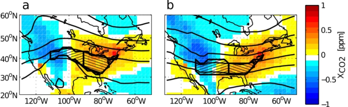
Rather than use geographically defined regions to average the data, we define the north-south boundaries based on potential temperature,θ. In simulations with zonally

10

uniform surface fluxes,X_CO

2 is tightly correlated with potential temperature,θ

(Keppel-Aleks et al. (2011), their Fig. 12). Therefore, in absence of zonal assymetry in fluxes, isentropic regions would yield contrasts of zero, while flux asymmetries introduced by fossil and biospheric fluxes would yield observable regional contrasts. To implement dy-namically defined regions, we fix the coordinates at the northeast and southeast edge

15

of the emission region and calculate the monthly meanθ at 700 hPa at these coordi-nates (Fig. 2). The potential temperature contours that intersect these verticies then define the northern and southern boundaries of the emission and upwind regions. The east-west boundaries are informed by the zonal anomaly inX_CO

2,fossil in AM2 and are

fixed on an annual basis. Although the geographic boundaries of the regions change

20

each month, this approach provides a semi-Lagrangian averaging framework. For In-dia, where wind direction reverses seasonally with the monsoon and where tempera-ture gradients are small, we cannot useθto define a dynamical region and instead use geographically fixed coordinates.

3 Data

25

We analyze ACOS-GOSATX_CO

2 data retrieved from spectra obtained between April

(7)

ACPD

12, 29887–29913, 2012

Title Page

Tables Figures

◭ ◮

Back Close

Full Screen / Esc

Discussion

P

a

per

|

Dis

cussion

P

a

per

|

Discussion

P

a

per

|

Discussio

n

P

a

per

|

Japanese Ministry of the Environment, the National Institute for Environmental Stud-ies, and the Japan Aerospace Exploration Agency. GOSAT samples the same location every three days and has a nadir footprint of 10.5 km diameter (86.6 km2area). Details about the retrieval method are provided by O’Dell et al. (2012). We primarily present results using ACOS-GOSAT v 2.9 retrievals, although we have also analyzed

prelimi-5

nary ACOS-GOSAT v 2.10 retrievals to test the sensitivity of our results to the retrieval. Because only data obtained over the land have been validated to date, we test our pre-dictions regarding regional contrasts over China and the eastern United States, where the corresponding upwind regions are over land. We also analyze contrasts for regions where we expect minimal contribution from fossil emissions, including Australia and

10

the upwind-of-China region, for which we average ACOS-GOSATX_CO

2 from a region

further upwind to calculate a regional ACOS-GOSATX_CO

2 contrast. We filter the data

and apply appropriate bias corrections as detailed in Wunch et al. (2011b). We also av-erage ACOS-GOSAT data obtained in target mode to determine “unique” data points and not over-weight observations over targeted regions.

15

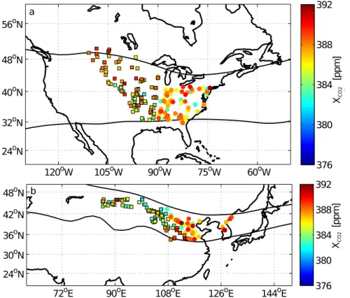
We define dynamically adaptive regions for averaging the ACOS-GOSAT data using the same method as for AM2. The eastern and western boundaries for the emission and upwind regions are the same as for AM2, and we use NCEP reanalysis potential temperature (Kalnay et al., 1996) to determine the north and south boundaries (Fig. 3). To estimate the potential sampling bias in the ACOS-GOSAT contrasts, we compare

20

the observations against AM2 sampled using two different approaches: at all gridboxes within the dynamically defined emission and upwind regions, and only at gridboxes containing ACOS-GOSAT retrievals. We average data from 2009–2011 to improve the statistics, assuming no interannual variability, a reasonable assumption for fossil fuel emissions between 2009 and 2011 (Boden et al., 2012). Although ground-based

ob-25

servations ofX_CO

2 show substantial interannual variability due to biospheric fluxes, we

do not attempt to account for the variability inX_CO

2,bio in the present study. To

com-pare with AM2, we have increased the simulated ChineseX_CO

(8)

ACPD

12, 29887–29913, 2012

Title Page

Tables Figures

◭ ◮

Back Close

Full Screen / Esc

Discussion

P

a

per

|

Dis

cussion

P

a

per

|

Discussion

P

a

per

|

Discussio

n

P

a

per

|

tagged ChineseX_CO

2,fossilcontrast to account for the increased emissions compared to

2007 (Boden et al., 2012).

4 Results

4.1 Simulations

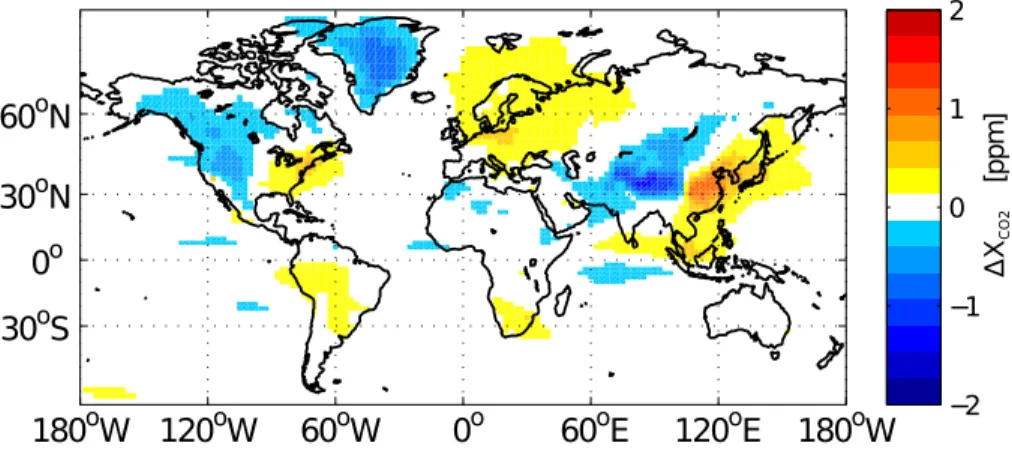
The signal in X_CO

2 from fossil fuel emissions is small. The enhancement in annual

5

meanX_CO

2,fossil at 2

◦ _{by 2.5}◦ _{resolution is at most 1.5 ppm above the zonal mean for}

any gridcell (Fig. 1). As expected, the largest anomalies are over regions with large fossil fuel emissions (e.g., the eastern United States, Europe, and China).

The regionalX_CO

2,fossilcontrasts scale with emissions for the six source regions

(Ta-ble 2). For regions with the largest emissions (eastern US, Europe, and China), fossil

10

fuel emissions impart a potentially detectable regional contrast of 0-2–0.8 ppm, while regions with smaller total emissions have a significantly smaller regionalX_CO

2,fossil

con-trast. Local fossil emissions account for a large fraction of theX_CO

2,fossilcontrast in the

simulations (Table 2). The contribution to theX_CO

2,fossil contrasts from foreign source

regions are close to zero, meaning that the contrasts primarily reflect local emissions,

15

although the China X_CO

2,fossil contrast is augmented by emissions from elsewhere in

Asia.

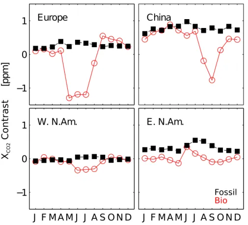
On a seasonal basis, the regional contrasts inX_CO

2owing to fossil fuel emissions are

partially obscured even in the largest source regions by seasonally varying biospheric fluxes (Fig. 4). We do not show the contribution from ocean fluxes in AM2 since they

20

cause only small (well under 0.1 ppm) spatial variations in the column. Although the regional biospheric contrast is minimized by the use of the semi-Lagrangian averaging regions, growing season contrasts are of order 1 ppm for Europe and China, suggest-ing that the fossil fuel signal may be more clear in satellite data acquired outside the growing season.

(9)

ACPD

12, 29887–29913, 2012

Title Page

Tables Figures

◭ ◮

Back Close

Full Screen / Esc

Discussion

P

a

per

|

Dis

cussion

P

a

per

|

Discussion

P

a

per

|

Discussio

n

P

a

per

|

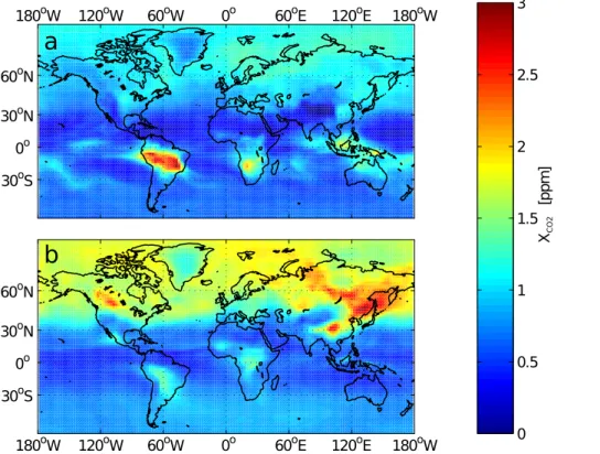
Seasonal patterns inX_CO

2variability on synoptic scales also impacts the detectability

of contrasts in the fossil component ofX_CO

2. Biospheric fluxes primarily determine the

large scale gradient inX_CO

2, and advection of those gradients is the dominant source of

temporal variations inX_CO

2(Keppel-Aleks et al., 2011). While these variations provide a

useful tool to infer the large scale gradient inX_CO

2 when measured at a single site on a

5

continuous basis (such as from ground-based TCCON observatories), they complicate the interpretation of most satellite data, where observations are made at low temporal resolution. Synoptic variability in CO2is relatively small when large scale gradients are

small, but during the Northern Hemisphere growing season, synoptic activity induces RMS variability of order 3 ppm in the Northern Hemisphere midlatitudes focused along

10

the storm tracks, coincident with the regions in which substantial fossil fluxes occur (Fig. 5a–b). That the variations are smaller outside the growing season again suggests that the signal from fossil fluxes should be easier to diagnose in winter and autumn.

As expected for a passive tracer like CO₂, the constructed contrasts scale linearly with emissions. TheX_CO

2,fossilcontrasts for the six study regions increase by a factor of

15

2.00±0.05 when we simulateXCO₂,fossilfields with doubled global emissions. To further

verify linearity, we simulatedX_CO

2,fossil with doubled Chinese emissions. The resulting

contrasts were equal to the sum of the contrasts from base global emissions plus the contrasts from tagged Chinese emissions.

The residence time of fossil CO₂ within the defined emission region a_ffects the

ex-20

pected contrast. To test the sensitivity of the contrast to the residence time, we run the AM2 with fossil fluxes emitted in the free troposphere (650±50 hPa) rather than at the surface, which is likely an overestimate of the potential error in the simulated re-gional signal if vertical mixing rates are underestimated. The mean contrasts decrease by 30±10 % due to faster transport times of CO2away from the emission region. The

25

(10)

ACPD

12, 29887–29913, 2012

Title Page

Tables Figures

◭ ◮

Back Close

Full Screen / Esc

Discussion

P

a

per

|

Dis

cussion

P

a

per

|

Discussion

P

a

per

|

Discussio

n

P

a

per

|

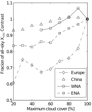
The regional contrasts described above are computed from all gridboxes in the dy-namically defined regions regardless of cloud cover; in reality, remote sensing obser-vations ofX_CO

2,fossil are obtained only under clear-sky conditions which may induce a

bias in the regional contrasts. In AM2, the calculated regional fossil contrasts gener-ally decrease relative to the all-sky value when gridboxes with fractional cloud cover

5

above a threshold value are excluded from the regional averages (Fig. 6). The sensi-tivity varies substantially by region: for instance, the regional contrast over China and western North America decreases by less than 10 % when the cloud threshold is 50 %. In contrast, eastern North America and European regional fossil contrasts decrease by 20 % and 30 % with a 50 % cloud threshold. The cloud bias in AM2 simulations

10

results from clouds preferentially obscuring AM2 gridboxes whose X_CO

2,fossil

concen-trations are higher than the regional average. AM2 does not include aerosols, which would limit satellite retrievals similarly to clouds. HighX_CO

2,fossilmay be correlated with

high aerosol optical depth, which could further reduce observed regionalX_CO

2,fossil

con-trasts.

15

4.2 Comparison with ACOS-GOSAT data

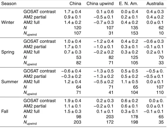
The regional contrasts in ACOS-GOSAT data are of the magnitude we expect based on the AM2 simulations and generally scale with fossil fuel emissions for the major emis-sion regions (China and the eastern United States, Table 3). The comparison reveals two initial complications. First, the sampling bias for AM2 is large (up to 1 ppm)

be-20

tween a GOSAT-like sampling and a spatially and temporally complete sampling (e.g., the spring contrast over China). Second, the upwind-of-China and Australia regions, which were chosen to test the agreement between AM2 and observations where fos-sil emissions are small, show significant regional contrasts likely owing to biospheric patterns. As expected based on the simulations, these biases are minimized during

25

(11)

ACPD

12, 29887–29913, 2012

Title Page

Tables Figures

◭ ◮

Back Close

Full Screen / Esc

Discussion

P

a

per

|

Dis

cussion

P

a

per

|

Discussion

P

a

per

|

Discussio

n

P

a

per

|

In winter and autumn, the comparison between ACOS-GOSAT observations and AM2 agrees well for the eastern United States when we sample AM2 only where we have ACOS-GOSAT observations. For China, the comparison between observations and simulations is more favorable when AM2 is sampled everywhere within the emis-sion and upwind regions. Still, the observed ACOS-GOSAT enhancement over the

Chi-5

nese emission region is larger than that predicted by AM2, even with a 25 % increase added to the simulatedX_CO

2,fossilcontrast. This discrepancy could be tied to issues with

either the ACOS-GOSAT observations or the simulations. An aerosol-induced X_CO

2

bias may have inflated the observed contrast, or an underestimate in CDIAC Chinese fossil fuel emissions (e.g., Zhao et al., 2012 and Guan et al., 2012) or CASA NEE may

10

have resulted in a biased simulated contrast. The regional contrast observed over the source and upwind regions of China is similar for all three seasons outside the Northern Hemisphere growing season. It is worth noting that only a small dataset that passed all the appropriate quality flags was used to calculate the regional contrasts (Table 3).

We tested the effect of the retrieval by computing the seasonal contrasts using

non-15

bias corrected ACOS-GOSAT v 2.9 retrievals and found that the observed contrasts changed by±0.2–0.5 ppm, with no consistent sign difference. We also calculated re-gional contrasts using preliminary ACOS-GOSAT v 2.10 retrievals with more restrictive quality flags compared to v 2.09, reducing the number of retrievals used to compute the regional averages. The calculated contrasts agreed to those presented in Table 3 to

20

within the standard errors; however the error bars were much larger due to the reduced number of data.

5 Conclusions

Our analysis with simulatedX_CO

2 fields suggests that fossil CO2emissions leave

dis-cernible signatures on globalX_CO

2 fields, although these signatures are small and their

25

(12)

ACPD

12, 29887–29913, 2012

Title Page

Tables Figures

◭ ◮

Back Close

Full Screen / Esc

Discussion

P

a

per

|

Dis

cussion

P

a

per

|

Discussion

P

a

per

|

Discussio

n

P

a

per

|

changes in observedX_CO

2 contrasts could be used to monitor changes in fossil

emis-sions.

Two year seasonal averages of regional contrasts in the ACOS-GOSAT data scale with our expectations based on AM2 simulations, even though the contrasts did not quantitatively agree with the simulations year-round. At least some of the di_fference

5

comes from sampling bias: regional contrasts are different in the model when we sam-ple only at locations with ACOS-GOSAT retrievals versus when we samsam-ple everywhere within the dynamical boundaries. The remaining disagreement could be due to di_ff er-ences in the fossil fluxes underlying the model and actual emissions, due to differences in biospheric fluxes, or due to bias in the observations due to cloud or aerosol

contam-10

ination. The emissions underlying AM2 in our experiments are based on CDIAC flux estimates, which Guan et al. (2012) estimate are 10 % below Chinese emissions esti-mated from province-level statistics and that Zhao et al. (2012) estimate are 10 % be-low emissions determined from a bottom-up Monte Carlo model. The simulations also show that regional biospheric enhancements will potentially obscure fossil fuel

signa-15

tures, consistent with observations of CO2made in China and Korea which show that

up to 50 % of the boundary layer enhancement in polluted regions owes to biospheric emissions (Turnbull et al., 2011b).

Although the initial comparison presented here between simulations and observa-tions demonstrates that estimating fossil fuel emissions from space will be difficult, our

20

results provide direction for makingX_CO

2 a more useful observation for validating fossil

fuel emissions. Both the sampling bias in AM2 (Table 3) and the cloud bias (Fig. 6) point toward footprint size as a key design factor in the utility of satellite observations for fossil fuel emissions monitoring at policy relevant accuracy. OCO-2, with a footprint 40 times smaller than that of GOSAT, may be an easier data set from which to diagnose

25

(13)

ACPD

12, 29887–29913, 2012

Title Page

Tables Figures

◭ ◮

Back Close

Full Screen / Esc

Discussion

P

a

per

|

Dis

cussion

P

a

per

|

Discussion

P

a

per

|

Discussio

n

P

a

per

|

Our results show that the regional contrasts estimated from bias-corrected ACOS-GOSAT data agree better with predictions from AM2, which underscore the importance of careful characterization of satellite retrievals and of an accurate bias correction. We note optimistically that retrievals from GOSAT will likely improve as the retrieval algorithm is further developed and potential sources of bias are better characterized.

5

The launch of OCO-2 and other satellites will provide more, and potentially better, datasets with which to work. OCO-2 requires single-sounding precision of 1 ppm (Miller et al., 2007; Wunch et al., 2011b), slightly better than the single-sounding precision of 1.0–1.5 ppm for ACOS-GOSAT data (O’Dell et al., 2012).

The method described here is certainly not the most precise method to infer

emis-10

sions rates fromX_CO

2 observations. Techniques such as data assimilation or flux

in-versions should provide more precise flux estimates and will be necessary to account for interannual variability in natural CO2fluxes, which we have ignored in this analysis.

Moreover, analysis of how concomitant changes in land fluxes and ocean fluxes will accompany decadal-scale increases in fossil fuel emissions is necessary as coherent

15

regional changes may obscure detection of fossil signatures. The methodology pre-sented in this paper does represent one tool that can be used in conjunction with other observations at other spatial scales to move toward national-level emissions verifica-tion.

Acknowledgements. The satellite data were produced by the ACOS/OCO-2 project at the Jet

20

Propulsion Laboratory, California Institute of Technology. The spectra were acquired by the GOSAT project. Support for this work from NASA grants NNX11AG016 and NNX08AI86G is gratefully acknowledged. We acknowledge the Keck Institute for Space Studies for inspiring this study. GKA acknowledges support from a NOAA Climate and Global Change postdoctoral fellowship.

(14)

ACPD

12, 29887–29913, 2012

Title Page

Tables Figures

◭ ◮

Back Close

Full Screen / Esc

Discussion

P

a

per

|

Dis

cussion

P

a

per

|

Discussion

P

a

per

|

Discussio

n

P

a

per

|

References

Anderson, J. L., Balaji, V., Broccoli, A. J., Cooke, W. F., Delworth, T. L., Dixon, K. W., Donner, L. J., Dunne, K. A., Freidenreich, S. M., Garner, S. T., Gudgel, R. G., Gordon, C. T., Held, I. M., Hemler, R. S., Horowitz, L. W., Klein, S. A., Knutson, T. R., Kushner, P. J., Langenhost, A. R., Lau, N. C., Liang, Z., Malyshev, S. L., Milly, P. C. D., Nath, M. J., Ploshay, J. J., Ramaswamy,

5

V., Schwarzkopf, M. D., Shevliakova, E., Sirutis, J. J., Soden, B. J., Stern, W. F., Thompson, L. A., Wilson, R. J., Wittenberg, A. T., and Wyman, B. L.: The new GFDL global atmosphere and land model AM2-LM2: Evaluation with prescribed SST simulations, J. Climate, 17, 4641– 4673, 2004. 29891

Andres, R. J., Gregg, J. S., Losey, L., Marland, G., and Boden, T. A.: Monthly, global emissions

10

of carbon dioxide from fossil fuel consumption, Tellus B, 63, 309–327, doi:10.1111/j.1600-0889.2011.00530.x, 2011. 29891

Andres, R. J., Marland, G., Fung, I., and Matthews, E.: A Distribution of Carbon Dioxide Emis-sions From Fossil Fuel Consumption and Cement Manufacture, Global Biogeochem. Cy., 10, 419–429, doi:10.1029/96GB01523, 1996.

15

Boden, T., Marland, G., and Andres, R.: Global, regional, and national fossil-fuel CO₂ emis-sions, Carbon Dioxide Information Analysis Center, Oak Ridge National Laboratory, US Department of Energy, Oak Ridge, Tenn., USA, doi:10.3334/CDIAC/00001 V2012, 2012. 29891, 29893, 29894

Buchwitz, M., de Beek, R., No ¨el, S., Burrows, J. P., Bovensmann, H., Bremer, H., Bergamaschi,

20

P., K ¨orner, S., and Heimann, M.: Carbon monoxide, methane and carbon dioxide columns retrieved from SCIAMACHY by WFM-DOAS: year 2003 initial data set, Atmos. Chem. Phys., 5, 3313–3329, doi:10.5194/acp-5-3313-2005, 2005. 29889

Corbin, K. D., Denning, A. S., and Gurney, K. R.: The space and time impacts on US regional atmospheric CO₂concentrations from a high resolution fossil fuel CO₂emissions inventory,

25

Tellus B, 62, 506–511, doi:10.1111/j.1600-0889.2010.00480.x, 2010. 29889

Duren, R. M. and Miller, C. E.: Measuring the carbon emissions of megacities, Nature Clim. Change, 2, 560–562, 2012. 29889

EIA: International Energy Outlook 2009, Tech. rep., US Department of Energy, 2009.

Friedlingstein, P., Houghton, R. A., Marland, G., Hackler, J., Boden, T. A., Conway, T. J.,

30

(15)

ACPD

12, 29887–29913, 2012

Title Page

Tables Figures

◭ ◮

Back Close

Full Screen / Esc

Discussion

P

a

per

|

Dis

cussion

P

a

per

|

Discussion

P

a

per

|

Discussio

n

P

a

per

|

Gregg, J. S. and Andres, R. J.: A method for estimating the temporal and spatial patterns of carbon dioxide emissions from national fossil-fuel consumption, Tellus B, 60, 1–10, 2008. 29891

Guan, D., Liu, Z., Geng, Y., Lindner, S., and Hubacek, K.: The gigatonne gap in China’s car-bon dioxide inventories, Nature Clim. Change, 2, 672–675, doi:10.1038/nclimate1560, 2012.

5

29897, 29898

Gurney, K. R., Law, R. M., Denning, A. S., Rayner, P. J., Baker, D., Bousquet, P., Bruhwiler, L., Chen, Y.-H., Ciais, P., Fan, S., Fung, I. Y., Gloor, M., Heimann, M., Higuchi, K., John, J., Maki, T., Maksyutov, S., Masarie, K., Peylin, P., Prather, M., Pak, B. C., Randerson, J., Sarmiento, J., Taguchi, S., Takahashi, T., and Yuen, C.-W.: Towards robust regional

esti-10

mates of CO₂sources and sinks using atmospheric transport models, Nature, 415, 626–630, doi:10.1038/415626a, 2002. 29889

Gurney, K. R., Mendoza, D. L., Zhou, Y. Y., Fischer, M. L., Miller, C. C., Geethakumar, S. and Du Can, S. D.: High resolution fossil fuel combustion CO₂emission fluxes for the United States, Environ. Sci. Technol., 43, 5535–5541, 2009. 29890

15

Kalnay, E., Kanamitsu, M., Kistler, R., Collins, W., Deaven, D., Gandin, L., Iredell, M., Saha, S., White, G., Woollen, J., Zhu, Y., Chelliah, M., Ebisuzaki, W., Higgins, W., Janowiak, J., Mo, K. C., Ropelewski, C., Wang, J., Leetmaa, A., Reynolds, R., Jenne, R., and Joseph, D.: The NCEP/NCAR 40-year reanalysis project, B. Am. Meteorol. Soc., 77, 437–471, 1996. 29893 Keppel-Aleks, G., Wennberg, P. O., and Schneider, T.: Sources of variations in total column

20

carbon dioxide, Atmos. Chem. Phys., 11, 3581–3593, doi:10.5194/acp-11-3581-2011, 2011. 29892, 29895

Keppel-Aleks, G., Wennberg, P. O., Washenfelder, R. A., Wunch, D., Schneider, T., Toon, G. C., Andres, R. J., Blavier, J.-F., Connor, B., Davis, K. J., Desai, A. R., Messerschmidt, J., Notholt, J., Roehl, C. M., Sherlock, V., Stephens, B. B., Vay, S. A., and Wofsy, S. C.: The imprint of

25

surface fluxes and transport on variations in total column carbon dioxide, Biogeosciences, 9, 875–891, doi:10.5194/bg-9-875-2012, 2012. 29891

Kort, E. A., Frankenberg, C., Miller, C. E., and Oda, T.: Space-based observations of megacity carbon dioxide, Geophys. Res. Lett., 39, L17806, doi:10.1029/2012GL052738, 2012. 29889 Le Qu ´er ´e, C., Raupach, M. R., Canadell, J. G., Marland, G., Bopp, L., Ciais, P., Conway, T. J.,

30

(16)

ACPD

12, 29887–29913, 2012

Title Page

Tables Figures

◭ ◮

Back Close

Full Screen / Esc

Discussion

P

a

per

|

Dis

cussion

P

a

per

|

Discussion

P

a

per

|

Discussio

n

P

a

per

|

S., Takahashi, T., Viovy, N., van der Werf, G. R., and Woodward, F. I.: Trends in the sources and sinks of carbon dioxide, Nat. Geosci., 2, 831–836, 2009. 29888

Marland, G. and Rotty, R. M.: Carbon-dioxide Emissions From Fossil-fuels - A Procedure For Estimation and Results For 1950–1982, Tellus B, 36, 232–261, 1984. 29891

Meehl, G. A., Stocker, T. F., Collins, W. D., Friedlingstein, P., Gaye, A. T., Gregory, J. M., Kitoh,

5

A., Knutti, R., Murphy, J. M., Noda, A., Raper, S. C. B., Watterson, I. G., Weaver, A. J., and Zhao, C.: Global Climate Projections. In Climate Change 2007: The Physical Science Basis. Contribution of Working Group I to the Fourth Assessment Report of the Intergovernmental Panel on Climate Change, Cambridge University Press, 2007. 29888

Miller, C. E., Crisp, D., DeCola, P. L., Olsen, S. C., Randerson, J. T., Michalak, A. M., Alkhaled,

10

A., Rayner, P., Jacob, D. J., Suntharalingam, P., Jones, D. B. A., Denning, A. S., Nicholls, M. E., Doney, S. C., Pawson, S., Boesch, H., Connor, B. J., Fung, I. Y., O’Brien, D., Salawitch, R. J., Sander, S. P., Sen, B., Tans, P., Toon, G. C., Wennberg, P. O., Wofsy, S. C., Yung, Y. L., and Law, R. M.: Precision requirements for space-based X_CO

2 data, J. Geophys. Res., 112, D10314, doi:10.1029/2006JD007659, 2007. 29899

15

Newman, S., Jeong, S., Fischer, M. L., Xu, X., Haman, C. L., Lefer, B., Alvarez, S., Rap-penglueck, B., Kort, E. A., Andrews, A. E., Peischl, J., Gurney, K. R., Miller, C. E., and Yung, Y. L.: Diurnal tracking of anthropogenic CO₂ emissions in the Los Angeles basin megacity during spring, 2010, Atmos. Chem. Phys. Discuss., 12, 5771–5801, doi:10.5194/acpd-12-5771-2012, 2012. 29889

20

NRC: Verifying Greenhouse Gas Emissions: Methods to Support International Climate Agree-ments, National Academies Press, 2010. 29888

O’Dell, C. W., Connor, B., B ¨osch, H., O’Brien, D., Frankenberg, C., Castano, R., Christi, M., El-dering, D., Fisher, B., Gunson, M., McDuffie, J., Miller, C. E., Natraj, V., Oyafuso, F., Polonsky, I., Smyth, M., Taylor, T., Toon, G. C., Wennberg, P. O., and Wunch, D.: The ACOS CO₂

re-25

trieval algorithm – Part 1: Description and validation against synthetic observations, Atmos. Meas. Tech., 5, 99–121, doi:10.5194/amt-5-99-2012, 2012. 29893, 29899

Olsen, S. C. and Randerson, J. T.: Di_fferences between surface and column atmo-spheric CO₂ and implications for carbon cycle research, J. Geophys. Res., 109, D02301, doi:10.1029/2003JD003968, 2004. 29891

30

(17)

ACPD

12, 29887–29913, 2012

Title Page

Tables Figures

◭ ◮

Back Close

Full Screen / Esc

Discussion

P

a

per

|

Dis

cussion

P

a

per

|

Discussion

P

a

per

|

Discussio

n

P

a

per

|

Peters, W., Jacobson, A. R., Sweeney, C., Andrews, A. E., Conway, T. J., Masarie, K., Miller, J. B., Bruhwiler, L. M. P., P ´etron, G., Hirsch, A. I., Worthy, D. E. J., van der Werf, G. R., Randerson, J. T., Wennberg, P. O., Krol, M. C., and Tans, P. P.: An atmospheric perspective on North American carbon dioxide exchange: CarbonTracker, P. Natl. Acad. Sci., 104, 18925– 18930, doi:10.1073/pnas.0708986104, 2007. 29889

5

Randerson, J. T., Thompson, M. V., Conway, T. J., Fung, I. Y., and Field, C. B.: The contribution of terrestrial sources and sinks to trends in the seasonal cycle of atmospheric carbon dioxide, Global Biogeochem. Cy., 11, 535–560, 1997. 29891

Suntharalingam, P., Jacob, D. J., Palmer, P. I., Logan, J. A., Yantosca, R. M., Xiao, Y., Evans, M. J., Streets, D. G., Vay, S. L., and Sachse, G. W.: Improved quantification of Chinese

10

carbon fluxes using CO₂/CO correlations in Asian outflow, J. Geophys. Res., 109, D18S18, doi:10.1029/2003JD004362, 2004.

Takahashi, T., Sutherland, S. C., Sweeney, C., Poisson, A., Metzl, N., Tilbrook, B., Bates, N., Wanninkhof, R., Feely, R. A., Sabine, C., Olafsson, J., and Nojiri, Y.: Global sea-air CO₂ flux based on climatological surface ocean pCO₂, and seasonal biological and temperature

15

effects, Deep-sea Res. Part II, 49, 1601–1622, 2002. 29892

Turnbull, J. C., Karion, A., Fischer, M. L., Faloona, I., Guilderson, T., Lehman, S. J., Miller, B. R., Miller, J. B., Montzka, S., Sherwood, T., Saripalli, S., Sweeney, C., and Tans, P. P.: Assessment of fossil fuel carbon dioxide and other anthropogenic trace gas emissions from airborne measurements over Sacramento, California in spring 2009, Atmos. Chem. Phys.,

20

11, 705–721, doi:10.5194/acp-11-705-2011, 2011. 29889

Turnbull, J. C., Tans, P. P., Lehman, S. J., Baker, D., Conway, T. J., Chung, Y. S., Gregg, J., Miller, J. B., Southon, J. R., and Zhou, L.-X.: Atmospheric observations of carbon monoxide and fossil fuel CO₂ emissions from East Asia, J. Geophys. Res., 116, D24306, doi:10.1029/2011JD016691, 2011b. 29898

25

Wunch, D., Wennberg, P. O., Toon, G. C., Keppel-Aleks, G., and Yavin, Y. G.: Emissions of greenhouse gases from a North American megacity, Geophys. Res. Lett., 36, L15810, doi:10.1029/2009GL039825, 2009. 29889

Wunch, D., Toon, G. C., Wennberg, P. O., Wofsy, S. C., Stephens, B. B., Fischer, M. L., Uchino, O., Abshire, J. B., Bernath, P., Biraud, S. C., Blavier, J.-F. L., Boone, C., Bowman, K. P.,

30

(18)

ACPD

12, 29887–29913, 2012

Title Page

Tables Figures

◭ ◮

Back Close

Full Screen / Esc

Discussion

P

a

per

|

Dis

cussion

P

a

per

|

Discussion

P

a

per

|

Discussio

n

P

a

per

|

Robinson, J., Roehl, C. M., Sawa, Y., Sherlock, V., Sweeney, C., Tanaka, T., and Zondlo, M. A.: Calibration of the Total Carbon Column Observing Network using aircraft profile data, Atmos. Meas. Tech., 3, 1351–1362, doi:10.5194/amt-3-1351-2010, 2010.

Wunch, D., Toon, G., J.-F. L, Blavier, Washenfelder, R., Notholt, J., Connor, B., Griffith, D., Sherlock, V., and Wennberg, P.: The Total Carbon Column Observing Network, Phil. Trans.

5

R. Soc. A, 369, 2087–2112, 2011. 29889

Wunch, D., Wennberg, P. O., Toon, G. C., Connor, B. J., Fisher, B., Osterman, G. B., Franken-berg, C., Mandrake, L., O’Dell, C., Ahonen, P., Biraud, S. C., Castano, R., Cressie, N., Crisp, D., Deutscher, N. M., Eldering, A., Fisher, M. L., Griffith, D. W. T., Gunson, M., Heikkinen, P., Keppel-Aleks, G., Kyr ¨o, E., Lindenmaier, R., Macatangay, R., Mendonca, J., Messerschmidt,

10

J., Miller, C. E., Morino, I., Notholt, J., Oyafuso, F. A., Rettinger, M., Robinson, J., Roehl, C. M., Salawitch, R. J., Sherlock, V., Strong, K., Sussmann, R., Tanaka, T., Thompson, D. R., Uchino, O., Warneke, T., and Wofsy, S. C.: A method for evaluating bias in global measurements of CO₂ total columns from space, Atmos. Chem. Phys., 11, 12317–12337, doi:10.5194/acp-11-12317-2011, 2011. 29893, 29899

15

Yokota, T., Oguma, H., Morino, I., and Inoue, G.: A nadir looking SWIR FTS to monitor CO₂ col-umn density for Japanese GOSAT project, Proc. Twenty-fourth Int. Sympo. on Space Tech-nol. and Sci. (Selected Papers), 887–889, 2004. 29889

Zhao, Y., Nielsen, C. P., and McElroy, M. B.: China’s CO2 emissions estimated from the bottom up: Recent trends, spatial distributions, and quantification of uncertainties, Atmos. Environ.,

20

(19)

ACPD

12, 29887–29913, 2012

Title Page

Tables Figures

◭ ◮

Back Close

Full Screen / Esc

Discussion

P

a

per

|

Dis

cussion

P

a

per

|

Discussion

P

a

per

|

Discussio

n

P

a

per

|

Table 1.Source regions for fossil fuel CO₂. The integrated emissions for 2007 are from Andres et al. (2011) and are used for AM2 simulations.

Emission Region Latitude Longitude 2007 emissions [Pg C yr−1

]

Europe 32–65◦_N ₂₀◦_W–28◦_E _1.2

India 7–33◦_N _68–88◦_E _0.4

China 20–48◦_N _100–135◦_E _2.1

W. N. Am 30–55◦_N _235–250◦_E _0.3

E. N. Am 25–55◦N 250–300◦E 1.4

(20)

ACPD

12, 29887–29913, 2012

Title Page

Tables Figures

◭ ◮

Back Close

Full Screen / Esc

Discussion

P

a

per

|

Dis

cussion

P

a

per

|

Discussion

P

a

per

|

Discussio

n

P

a

per

|

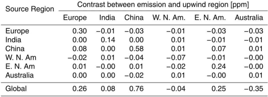
Table 2. X_CO

2,fossilcontrast [ppm] from regional emissions during October – November. We use dynamically adaptive emission and upwind regions to calculate the contrasts, except for India where we defined stationary averaging boxes.

Source Region Contrast between emission and upwind region [ppm] Europe India China W. N. Am. E. N. Am. Australia

Europe 0.30 −0.01 −0.03 −0.01 −0.03 −0.03

India 0.00 0.14 0.00 0.01 −0.01 −0.01

China 0.08 0.00 0.58 0.01 0.07 0.01

W. N. Am ₋0.02 0.01 ₋0.04 ₋0.07 ₋0.01 ₋0.00

E. N. Am 0.01 ₋0.00 0.01 ₋0.02 0.24 ₋0.00

Australia 0.00 0.00 ₋0.02 0.01 ₋0.00 0.01

(21)

ACPD

12, 29887–29913, 2012

Title Page

Tables Figures

◭ ◮

Back Close

Full Screen / Esc

Discussion

P

a

per

|

Dis

cussion

P

a

per

|

Discussion

P

a

per

|

Discussio

n

P

a

per

|

Table 3.X_CO

2 contrast [ppm] for ACOS GOSAT data and AM2 simulations. The AM2 partial contrast is sampled coincidently with GOSAT data. AM2 full contrasts average all model grid-boxes within the dynamically defined regions for all days within the season. GOSAT data are averaged for two years across four seasons: winter (January–February), spring (April–May), summer (July–August), and fall (October–November). The number of points in the ACOS emis-sion and upwind region are listed seasonally.

Season China China upwind E. N. Am. Australia

Winter

GOSAT contrast 1.7±0.4 0.1±0.6 0.0±0.4 0.4±0.3 AM2 partial 0.9±0.1 −0.5±0.1 0.2±0.1 0.4±0.2 AM2 full 1.4_±0.2 ₋0.7_±0.3 0.4_±0.2 0.0_±0.1

N 120 107 135 62

N_upwind 107 31 153 10

Spring

GOSAT contrast 1.0_±0.4 ₋1.2_±0.4 0.4_±0.2 ₋0.6_±0.3 AM2 partial 1.7_±0.1 ₋1.0_±0.1 0.3_±0.1 ₋0.1_±0.1 AM2 full 0.7±0.3 −0.2±0.2 0.3±0.2 0.2±0.1

N 53 82 125 70

N_upwind 82 71 105 33

Summer

GOSAT contrast ₋0.6_±0.4 ₋1.3_±0.5 0.5_±0.5 ₋0.5_±0. AM2 partial ₋0.3_±0.2 ₋1.3_±0.2 0.5_±0.2 ₋0.5_±0.1 AM2 full 1.2_±0.4 ₋0.5_±0.2 1.1_±0.5 0.0_±0.1

N 64 71 65 107

N_upwind 71 41 104 110

Fall

GOSAT contrast 1.9_±0.4 0.2_±0.3 0.6_±0.2 0.0_±0. AM2 partial 1.1_±0.1 ₋0.2_±0.1 0.6_±0.1 0.0_±0.1 AM2 full 1.5_±0.3 0.1_±0.1 0.3_±0.1 ₋0.1_±0.1

N 98 203 178 65

(22)

ACPD

12, 29887–29913, 2012

Title Page

Tables Figures

◭ ◮

Back Close

Full Screen / Esc

Discussion

P

a

per

|

Dis

cussion

P

a

per

|

Discussion

P

a

per

|

Discussio

n

P

a

per

|

180oW 120oW 60oW 0o 60oE 120oE 180oW 30oS

0o 30oN 60oN

∆

[p

p

m

]

X

CO2

−2

−1 0 1 2

Fig. 1.Zonal meanX_CO

2,fossilAnomaly. FossilXCO2 fields from the AM2 GCM are averaged for one year and detrended by the zonal mean to more clearly show the influence of source regions on globalX_CO

(23)

ACPD

12, 29887–29913, 2012

Title Page

Tables Figures

◭ ◮

Back Close

Full Screen / Esc

Discussion

P

a

per

|

Dis

cussion

P

a

per

|

Discussion

P

a

per

|

Discussio

n

P

a

per

|

120oW 100oW 80oW 60oW

20oN 30oN 40oN 50oN 60oN

120oW 100oW 80oW 60oW

[p

p

m

]

XCO2

−1

−0.5

0 0.5 1

a

b

Fig. 2. (a)May and(b)November dynamically adaptive regions over eastern North America. The eastern and western edges of the emission and upwind regions are determined based on contrasts in simulatedX_CO

(24)

ACPD

12, 29887–29913, 2012

Title Page

Tables Figures

◭ ◮

Back Close

Full Screen / Esc

Discussion

P

a

per

|

Dis

cussion

P

a

per

|

Discussion

P

a

per

|

Discussio

n

P

a

per

|

72oE 90oE 108oE 126oE 144oE 24oN

30oN 36oN 42oN 48oN b

<

CO

2

>

[p

p

m

]

376 380 384 388 392

[ppm

]

376 380 384 388 392

XCO2

120oW 105oW 90oW 75oW 60oW

24oN 32oN 40oN 48oN 56oN

a

<

CO

2

>

[p

p

m

]

376 380 384 388 392

[p

p

m

]

376 380 384 388 392

XCO2

Fig. 3.October 2009–2010 GOSATX_CO

(25)

ACPD

12, 29887–29913, 2012

Title Page

Tables Figures

◭ ◮

Back Close

Full Screen / Esc

Discussion

P

a

per

|

Dis

cussion

P

a

per

|

Discussion

P

a

per

|

Discussio

n

P

a

per

|

−

1

0

1 Europe

China

J F M A M J J A S O N D

−

1

0

1 W. N.Am.

J F M A M J J A S O N D

E. N.Am.

[

ppm

]

X

CO2

Contrast

Fossil Bio

Fig. 4.Simulated regional contrast inX_CO

2,bio(red) andXCO2,fossil(black) for four source regions. The contrast inX_CO

(26)

ACPD

12, 29887–29913, 2012

Title Page

Tables Figures

◭ ◮

Back Close

Full Screen / Esc

Discussion

P

a

per

|

Dis

cussion

P

a

per

|

Discussion

P

a

per

|

Discussio

n

P

a

per

|

180oW 120oW 60oW 0o 60oE 120oE 180oW

30oS

0o

30oN

60oN

180oW 120oW 60oW 0o 60oE 120oE 180oW

30oS

0o

30oN

60oN

[p

p

m

]

X

CO2

0 0.5 1 1.5 2 2.5 3

a

b

Fig. 5.Simulated seasonal variability inX_CO

(27)

ACPD

12, 29887–29913, 2012

Title Page

Tables Figures

◭ ◮

Back Close

Full Screen / Esc

Discussion

P

a

per

|

Dis

cussion

P

a

per

|

Discussion

P

a

per

|

Discussio

n

P

a

per

|

20 40 60 80 100

0.5 0.6 0.7 0.8 0.9 1 1.1

Maximum cloud cover [%]

F

rac

ion

of

all

−

sk

y

X

CO2

Contrast

Europe

China

WNA

ENA

Fig. 6.Relative change in the simulatedX_CO