www.atmos-chem-phys.net/12/10353/2012/ doi:10.5194/acp-12-10353-2012
© Author(s) 2012. CC Attribution 3.0 License.
Chemistry
and Physics
Particulate sulfate ion concentration and SO
2
emission trends in the
United States from the early 1990s through 2010
J. L. Hand1, B. A. Schichtel2, W. C. Malm1, and M. L. Pitchford3
1Cooperative Institute for Research in the Atmosphere, Colorado State University, Fort Collins, Colorado, USA 2National Park Service, Cooperative Institute for Research in the Atmosphere, Colorado State University, Fort Collins,
Colorado, USA
3Desert Research Institute, Reno, Nevada, USA
Correspondence to:J. L. Hand ([email protected])
Received: 11 July 2012 – Published in Atmos. Chem. Phys. Discuss.: 3 August 2012 Revised: 12 October 2012 – Accepted: 23 October 2012 – Published: 7 November 2012
Abstract. We examined particulate sulfate ion
concentra-tions across the United States from the early 1990s through 2010 using remote/rural data from the Interagency Monitor-ing of Protected Visual Environments (IMPROVE) network and from early 2000 through 2010 using data from the Envi-ronmental Protection Agency’s (EPA) urban Chemical Spe-ciation Network (CSN). We also examined measured sul-fur dioxide (SO2) emissions from power plants from 1995
through 2010 from the EPA’s Acid Rain Program. The 1992– 2010 annual mean sulfate concentrations at long-term ru-ral sites in the United States have decreased significantly and fairly consistently across the United States at a rate of
−2.7 % yr−1(p <0.01). The short-term (2001–2010) annual
mean trend at rural sites was −4.6 % yr−1 (p <0.01) and
at urban sites (2002–2010) was−6.2 % yr−1(p<0.01).
An-nual total SO2emissions from power plants across the United
States have decreased at a similar rate as sulfate concentra-tions from 2001 to 2010 (−6.2 % yr−1,p <0.01),
suggest-ing a linear relationship between SO2 emissions and
aver-age sulfate concentrations. This linearity was strongest in the eastern United States and weakest in the West where power plant SO2emissions were lowest and sulfate concentrations
were more influenced by non-power-plant and perhaps inter-national SO2emissions. In addition, annual mean, short-term
sulfate concentrations decreased more rapidly in the East rel-ative to the West due to differences in seasonal trends at cer-tain regions in the West. Specifically, increased wintertime concentrations in the central and northern Great Plains and increased springtime concentrations in the western United States were observed. These seasonal and regional positive
trends could not be explained by changes in known local and regional SO2emissions, suggesting other contributing
influ-ences. This work implies that on an annual mean basis across the United States, air quality mitigation strategies have been successful in reducing the particulate loading of sulfate in the atmosphere; however, for certain seasons and regions, espe-cially in the West, current mitigation strategies appear insuf-ficient.
1 Introduction
Sulfate is an important secondary aerosol formed from pho-tochemical reactions of sulfur dioxide (SO2)emissions in the
atmosphere. In the United States it is a major contributor to the PM2.5mass, accounting for 30–60 % of the fine monthly
and terrestrial ecosystems (e.g., Lehmann and Gay, 2011), is active as cloud-condensation nuclei and in cloud microphys-ical processes (e.g., Petters et al., 2009), interacts directly with incoming shortwave radiation and thereby contributes to global cooling (e.g., Kiehl and Briegleb, 1993), and is poten-tially harmful to human health (e.g., Rohr and Wyzga, 2012). Regulatory and legislative mandates, such as Title IV of the 1990 Clean Air Act Amendment, were established to re-duce SO2 emissions in the United States. These mandates
have been successful and, from 1990 to 2010, total annual SO2 emissions in the United States have decreased 60 %
(U.S. EPA, 2011a). Reductions in SO2 emissions should
lower particulate sulfate concentrations in the atmosphere and precipitation (Lehmann and Gay, 2011). Reductions could also significantly lower PM2.5mass concentrations in
areas where sulfate is a dominant contributor, assisting goals in meeting the PM2.5and PM10 particulate matter National
Ambient Air Quality Standards (NAAQS). The effects of emission reductions on visibility degradation are addressed by the Regional Haze Rule (RHR), promulgated by the EPA in 1999 (U.S. EPA, 1999). Its goals include reducing the worst haze days in class I areas to natural levels by 2064. Sulfate contributes∼10–85 % of haze (Hand et al., 2011);
therefore, reductions in sulfate concentrations are important for achieving RHR goals. A recent examination of progress toward RHR goals was reported in Hand et al. (2011).
Trend analyses are needed to track progress toward reg-ulatory goals and to evaluate success of emission reduc-tion programs by understanding how ambient concentra-tions respond to changes in emissions. Trend analyses re-quire stable, long-term data sets obtained under consistent monitoring and analytical methods. The Interagency Mon-itoring of Protected Visual Environments (IMPROVE) pro-gram has monitored aerosol concentrations at remote and ru-ral sites in the United States since 1988; one of its main pur-poses is to support trends analyses. Trends in aerosol species such as sulfate and nitrate ions, carbonaceous aerosols, and gravimetric fine mass using IMPROVE data suggest that across the rural United States the annual mean concentra-tions of major aerosol species generally decreased through 2008 (e.g., Hand et al., 2011; Murphy et al., 2011). Ear-lier work by Malm et al. (2002) also demonstrated that IM-PROVE and CASTNet (Clean Air Status and Trends Net-work) sulfate concentrations decreased at most sites in the United States over a period of 10 yr (1988–1999), with the highest rates of decrease north of the Ohio River valley. Sul-fate concentrations at Whiteface Mountain, New York, re-portedly decreased by 59 % from 1979 through 2002 (Hu-sain et al., 2004). Blanchard et al. (2012) reports decreased annual mean sulfate concentrations ranging from 3.7 ± 1.1 to 6.2 ± 1.1 % yr−1from 1999 to 2010 at sites in the
south-eastern United States as part of the SEARCH (Southeast-ern Aerosol Research and Characterization) program. Malm et al. (2002) also examined SO2 emission data and found
that although it varied by region, sulfate concentrations and
SO2 emissions tracked fairly closely. Husain et al. (1998)
also reported a linear relationship between decreasing sul-fate concentrations and SO2emissions (Husain et al., 1998).
Reductions in sulfate concentrations in the atmosphere have decreased its concentration in precipitation as evidenced by Lehmann and Gay (2011). They performed trend analyses on precipitation data obtained from the National Atmospheric Deposition Program and demonstrated statistically signifi-cant decreases in sulfate concentrations in precipitation al-most everywhere in the United States from 1985 through 2009. Although annual mean concentrations of major aerosol species generally have decreased, this may not be the case for specific seasons or regions. For example, wintertime par-ticulate sulfate and nitrate ion concentrations have increased across the US northern and central Great Plains from 2000 through 2010 (Hand et al., 2012b).
Changes in sulfate concentrations over time are influenced not only by changes in local and regional emissions but also by changes in meteorology. Modeling studies to investigate the effects of future emission trends and meteorology on pollutant concentrations have been performed by several re-searchers. A study by Tai et al. (2010) showed that daily variations in meteorology can explain up to 50 % of PM2.5
variability due to temperature, relative humidity, precipita-tion, and circulation. Sulfate was positively correlated with temperature and relative humidity and negatively correlated with precipitation, suggesting that changes in these meteoro-logical variables can impact sulfate levels in the atmosphere. Further analysis by Tai et al. (2012) suggested these relation-ships were driven by synoptic transport in most locations.
and local emissions on sulfate trends requires a variety of data sets and tools, such as long-term observations, back tra-jectory analyses, and model simulations with changing emis-sions.
This paper builds on the previous work of Malm et al. (2002) by extending sulfate monthly, seasonal, and annual mean trend analyses through 2010 and by including both ru-ral and urban sites across the United States. Trends in sulfate concentrations and SO2 emissions from power plants were
evaluated to investigate their relationships and potential ef-fectiveness of emission control strategies. We also demon-strate that trends in seasonal mean concentrations can exhibit very different behaviors compared to trends in annual mean concentrations, highlighting the importance of understand-ing the impacts of meteorology and long-range transport to the interpretation of trends.
2 Data and methods
The IMPROVE program is a cooperative effort designed to monitor aerosol and visibility conditions in mandatory class I areas (Malm et al., 1994). The program began operating in remote areas in 1987 with approximately 30 sites and cur-rently operates 170 remote and some urban sites across the United States. The network collects 24-h samples every third day from midnight to midnight local time and concentrations are reported at local conditions. Additional details regard-ing IMPROVE samplregard-ing are provided by Malm et al. (1994) and Hand et al. (2011). All IMPROVE data, metadata, de-tailed descriptions of the network operations, data analysis, and visualization results are available for download from http://vista.cira.colostate.edu/IMPROVE/.
We used PM2.5sulfate ion data collected on nylon filters,
analyzed by ion chromatography, and artifact-corrected. Pre-cisions for sulfate ion concentrations were 4 % as reported by Hyslop and White (2008) for collocated data. White et al. (2005) estimated sulfate trend uncertainty due to mea-surement error as 1 % yr−1over a 5-yr period. We chose to
use sulfate ion data, rather than sulfur data as used by Malm et al. (2002), due to biases in sulfur concentrations derived from X-ray fluorescence as described by White (2009) and Hyslop et al. (2012). However, in the late 1990s inadvertent manufacturer changes to the nylon filter resulted in clogged filters during periods with high mass concentrations (Eldred, 2001). Loss of filters due to clogging primarily affected sites in the East, where 30 % or more of the samples were invali-dated during a given season, although some sites in the West were also affected. The issue was resolved by 2000. We de-termined that the missing samples resulted in biased monthly and annual mean sulfate concentrations because the clogging preferentially occurred during high mass events. To account for this bias, we replaced missing sulfate data before 2000 with sulfur concentrations that were scaled to sulfate mass.
The Speciated Trends Network (STN) and other urban monitoring sites are collectively known as the EPA’s Chemi-cal Speciation Network (CSN) and were deployed in the fall of 2000 (U.S. EPA, 2004), primarily in urban/suburban set-tings. The objectives of the CSN include tracking progress of emission reduction strategies through the characterization of trends. The CSN operates approximately 50 trend sites, with another∼150 sites operated by state, local, and tribal
agencies. The CSN collects 24-h samples every third or sixth day, on the same sampling schedule as IMPROVE. Data are reported at local conditions. We used PM2.5sulfate ion
con-centrations collected on nylon filters and analyzed by ion chromatography. The methods for collecting and analyzing sulfate ion concentrations are similar for the CSN and IM-PROVE network, with the exception that CSN does not cor-rect for artifacts and cold-ships filters. Comparisons of data from collocated sites from 2005 to 2008 suggested close agreement between CSN and IMPROVE sulfate ion concen-trations with a relative bias of 4.2 % (CSN higher) and a correlation of 0.99, and differences between urban and ru-ral sites were typically low (Hand et al., 2012a). CSN data can be downloaded from http://views.cira.colostate.edu/fed/ or http://www.epa.gov/ttn/airs/airsaqs/.
Annual SO2emission data by source category for the
en-tire United States were obtained from the EPA’s National Emissions Inventory (NEI) database (U.S. EPA, 2011a). However, examining SO2 emissions with finer spatial and
temporal resolution required obtaining SO2 emission data
from the EPA’s Clean Air Markets Division, Acid Rain Pro-gram (U.S. EPA, 2011b). As part of the Acid Rain ProPro-gram, the EPA established requirements for continuous emissions monitoring (CEM) of SO2 using SO2 pollutant
concentra-tion monitors on regulated facilities. Power plant emissions are the dominant source of total SO2emissions; in 2010
elec-tric utilities contributed∼65 % of NEI total SO2emissions.
SO2emissions reported for each facility within a given state
were aggregated to state-level monthly and annual total emis-sion rates from 1995 to 2010. SO2emissions discussed in this
paper refer to CEM SO2emissions.
Linear Theil regression (Theil, 1950) was performed on both the concentration and emission data. Fifty percent of the concentration data for given month and year had to be valid for a site to be considered “complete”, and 70 % of “complete” years were necessary for a trend calcula-tion over a given time period. We defined “trend” (% yr−1)
as the slope derived from the Theil regression divided by the median concentration value over the time period of the trend, multiplied by 100 %. Kendall tau statistics were used to determine the significance; a statistically significant trend was assumed at the 90th percentile significance level (p <0.10), meaning that there was a 90 % chance that the slope was not due to random chance. Trends were computed for monthly, seasonal, and annual means for sulfate concen-trations and monthly and annual total CEM SO2emissions.
for individual site trends and 1992–2010 for regional trends. IMPROVE and CSN short-term trends for individual sites were computed for 2000–2010, while regional trends were computed for 2001–2010 and 2002–2010 for IMPROVE and CSN trends, respectively (see Sect. 3.4).
3 Results
3.1 Long-term trends in sulfate ion concentrations
(1989–2010)
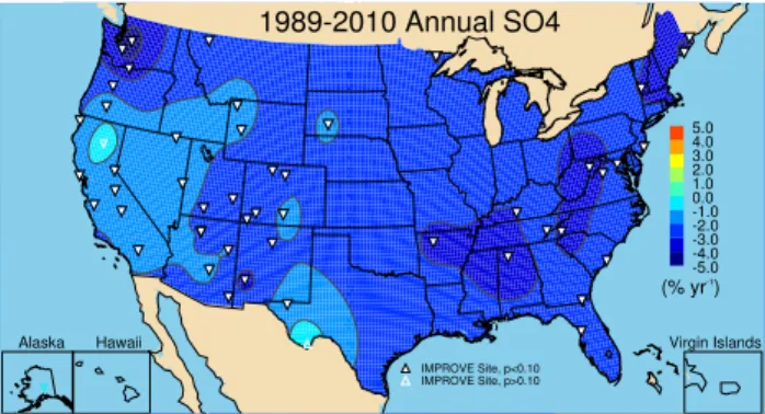
Long-term (1989–2010) annual mean sulfate trends at IM-PROVE sites are presented in Fig. 1. Isopleths were pro-duced by interpolating trend values at individual sites using a Kriging algorithm. Isopleths are meant to aid the visual-ization of spatial patterns and not for estimating trend val-ues between monitoring sites. Sites with statistically signif-icant trends (p <0.10) were represented by filled triangles that point upward or downward for increased or decreased concentrations, respectively. Sites with statistically insignifi-cant trends were represented by unfilled triangles. From 1989 to 2010 annual mean sulfate concentrations decreased at all but one of the 52 IMPROVE sites with 15 or more years of data; 49 sites corresponded to statistically significant trends (see Fig. 1). The largest decreases occurred in the East where sulfate generally decreased at a rate higher than−2 % yr−1.
In contrast, sulfate concentrations in the West decreased at a somewhat lower rate, especially closer to the coast. Long-term significant trends ranged from−4.8 % yr−1(p <0.01)
in Snoqualmie Pass, Washington (SNPA), to −1.0 % yr−1
(p=0.01) in Jarbidge, Nevada (JARB). Long-term trends
in annual mean concentrations for all sites are included in the Supplementary material. Notice from Fig. 1 that most of the earliest IMPROVE sites are located in the southwestern, western, and eastern United States, with a lack of sites in the central United States, Great Plains, and Great Lakes regions.
3.2 Short-term trends in sulfate ion concentrations
(2000–2010)
In 2000 the IMPROVE program expanded to 159 sites, fill-ing gaps in the spatial distribution in the above-mentioned regions. The addition of these IMPROVE sites, as well as CSN sites that began operation in 2000, allowed for trends to be computed with finer spatial resolution but over a shorter time period (2000–2010). As Hand et al. (2011, 2012a) demonstrated, urban sulfate concentrations were only slightly higher than neighboring rural sites; however, gen-erally good agreement suggested that urban and rural sites were influenced by similar regional sources. Since we fo-cused only on the changes in sulfate concentrations, some-what higher urban sulfate concentrations were of little con-sequence.
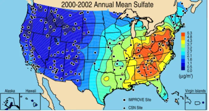
Annual mean sulfate concentrations from 2000–2002 and 2008–2010 are shown in Fig. 2a and b, respectively, for both
IMPROVE Site, p<0.10 IMPROVE Site, p>0.10
1989-2010 Annual SO4
-5.0 -4.0 -3.0 -2.0 -1.0 0.0 1.0 2.0 3.0 4.0 5.0
(% yr-1)
Alaska Hawaii Virgin Islands
Fig. 1. IMPROVE 1989–2010 trends (% yr−1) in annual mean
particulate sulfate ion concentrations. Triangles correspond to IM-PROVE sites; upward pointing triangles correspond to increased concentrations and vice versa. Trends with significance levels (p) less than 0.10 are considered significant.
IMPROVE and CSN data. These isopleth maps were gener-ated by interpolating data from both networks. Sulfate con-centrations were higher in the East where emissions were also highest (see Sect. 3.3). Comparisons of the two time pe-riods demonstrated considerable reductions in concentrations at both rural and urban sites from the early to late 2000s.
Trend results demonstrating these reductions in short-term (2000–2010) annual mean sulfate concentrations are presented in Fig. 3. A total of 281 sites are shown (154 and 127 IMPROVE and CSN sites, respectively, with at least eight years of complete data). Most of the sites had statistically significant trends (80 % and 94 % of IM-PROVE and CSN sites, respectively). Annual mean sul-fate concentrations significantly increased at only three IMPROVE sites; the largest occurred at Hawaii Volca-noes, Hawaii (HAVO, 9.4 % yr−1,p <0.01), Denali, Alaska
(DENA, 6.0 % yr−1, p
=0.04), and Fort Peck, Montana
(FOPE, 2.3 % yr−1, p
=0.06). The largest decrease in
ru-ral sulfate concentrations occurred in Martha’s Vineyard, Massachusetts (MAVI,−11.4 % yr−1,p <0.01). The range
in trends at the CSN sites were −10.5 % yr−1 in
Scran-ton, Pennsylvania (#420692006,p <0.01), to−1.3 % yr−1in
Portola, California (#060631009,p=0.012). Short-term an-nual mean trends for IMPROVE and CSN sites are reported in the Supplement.
Not only have annual mean sulfate concentrations de-creased nearly everywhere in the United States since 2000, but urban and rural concentrations decreased at similar rates, as indicated by the consistency in isopleths in Fig. 3 (this point will be discussed in more detail in Sect. 3.4). Concen-trations in the eastern United States decreased more rapidly than in the West, where sulfate ion concentrations were 5– 10 times lower (Fig. 2). To investigate these differences in more detail, we analyzed short-term seasonal mean trends to examine seasonal influence on the patterns seen in Fig. 3.
IMPROVE Site CSN Site
2000-2002 Annual Mean Sulfate
0.0 0.5 1.1 1.6 2.1 2.7 3.2 3.7 4.3 4.8 5.3
(µg/m3)
Alaska Hawaii Virgin Islands
Fig. 2a.IMPROVE and CSN 2000–2002 annual mean particulate sulfate ion concentrations. Circles correspond to IMPROVE sites and triangles correspond to CSN sites.
IMPROVE Site CSN Site
2008-2010 Annual Mean Sulfate
0.0 0.5 1.1 1.6 2.1 2.7 3.2 3.7 4.3 4.8 5.3
(µg/m3)
Alaska Hawaii Virgin Islands
Fig. 2b.IMPROVE and CSN 2008–2010 annual mean particulate sulfate ion concentrations. Circles correspond to IMPROVE sites and triangles correspond to CSN sites.
flat to positive (see Fig. 4a) in the northern Great Plains and Great Lakes regions, relative to other regions of the country, although most trends were insignificant. Positive winter trends in the Great Lake region were influenced by many CSN sites with increased January monthly mean con-centrations, such as at Rochester, Minnesota (#271095008, 7.1 % yr−1,p
=0.06), and Youngstown, Ohio (#390990014,
4.6 % yr−1, p
=0.03). These increased concentrations
oc-curred during what was historically associated with the sea-son of lowest sulfate concentrations during the year (Hand et al., 2012a).
In the northern Great Plains, winter trends were influenced by increased December monthly mean concentrations at a swath of sites extending southward from Montana into Ok-lahoma and parts of Texas. Hand et al. (2012b) reported on these trends only for IMPROVE sites, but sulfate concentra-tions at the few CSN sites within this area also increased. At the IMPROVE site at Fort Peck (FOPE), Montana, De-cember monthly mean sulfate concentrations increased at the steep rate of 17.5 % yr−1 (p
=0.06), beginning sharply in
2006. Sulfate concentrations increased steadily at 5.4 % yr−1
(p=0.03) at the CSN Omaha, Nebraska, site (#310550019). A less extensive spatial pattern occurred in February and was
IMPROVE Site, p<0.10 IMPROVE Site, p>0.10 CSN Site, p<0.10 CSN Site, p>0.10
2000-2010 Annual SO4
-5.0 -4.0 -3.0 -2.0 -1.0 0.0 1.0 2.0 3.0 4.0 5.0
(% yr-1)
Alaska Hawaii Virgin Islands
Fig. 3.IMPROVE and CSN 2000–2010 trends (% yr−1)in annual
mean particulate sulfate ion concentrations. White and magenta tri-angles correspond to IMPROVE and CSN sites, respectively; up-ward pointing triangles correspond to increased concentrations and vice versa. Trends with significance levels (p) less than 0.10 are considered significant.
absent in January. Intriguingly, sites within this swath were also associated with increased nitrate concentrations (Hand et al., 2012b). This area is associated with relatively low sulfate concentrations that historically peaked in spring and summer (Hand et al, 2012a); in 2010 the maximum sulfate concentrations occurred in winter at most of these sites. In other regions of the country the winter seasonal mean con-centrations significantly decreased at sites in the southeast-ern, northeastsoutheast-ern, and southwestern United States.
Springtime (MAM) trends in the West were noteworthy and contributed to the differences seen between the East and the West in the annual mean trends (Fig. 4b). Most of the sites in the West were associated with concentrations that decreased at a much lower rate, or even increased, relative to sites in the East. Positive trends were insignificant, most likely due a drop in concentrations in 2009 and 2010 that was common at many sites (see Sect. 3.4). This drop in concentra-tions had a strong influence on the trends, and in fact trends from 2000 to only 2008 were positive and statistically signif-icant at many sites. Increases in spring concentrations may have contributed to the shift in the maximum monthly sea-sonal concentrations from summer to spring at many north-and central-western sites since 2000 (Hnorth-and et al., 2012a).
IMPROVE Site, p<0.10 IMPROVE Site, p>0.10 CSN Site, p<0.10 CSN Site, p>0.10
2000-2010 Winter SO4
-5.0 -4.0 -3.0 -2.0 -1.0 0.0 1.0 2.0 3.0 4.0 5.0
(% yr-1)
Alaska Hawaii Virgin Islands
IMPROVE Site, p<0.10 IMPROVE Site, p>0.10 CSN Site, p<0.10 CSN Site, p>0.10
2000-2010 Spring SO4
-5.0 -4.0 -3.0 -2.0 -1.0 0.0 1.0 2.0 3.0 4.0 5.0
(% yr-1)
Alaska Hawaii Virgin Islands
IMPROVE Site, p<0.10 IMPROVE Site, p>0.10 CSN Site, p<0.10 CSN Site, p>0.10
2000-2010 Summer SO4
-5.0 -4.0 -3.0 -2.0 -1.0 0.0 1.0 2.0 3.0 4.0 5.0
(% yr-1
)
Alaska Hawaii Virgin Islands
IMPROVE Site, p<0.10 IMPROVE Site, p>0.10 CSN Site, p<0.10 CSN Site, p>0.10
2000-2010 Fall SO4
-5.0 -4.0 -3.0 -2.0 -1.0 0.0 1.0 2.0 3.0 4.0 5.0
(% yr-1
)
Alaska Hawaii Virgin Islands
Fig. 4.IMPROVE and CSN 2000–2010 trends (% yr−1)in seasonal mean particulate sulfate ion concentrations for(a)winter (DJF),(b)
spring (MAM),(c)summer (JJA) and(d)fall (SON). White and magenta triangles correspond to IMPROVE and CSN sites, respectively; upward pointing triangles correspond to increased concentrations and vice versa. Trends with significance levels (p) less than 0.10 are considered significant.
2000. Hawaii Volcanoes also experienced increased concen-trations for all seasonal means. Interestingly, concenconcen-trations dropped in 2010 for both sites, similar to other sites in the contiguous West discussed earlier.
3.3 Trends in SO2emissions
The 2000–2010 median total annual CEM SO2emissions for
each of the contiguous United States are shown in Fig. 5a. Emissions are plotted on a logarithmic scale in units of mil-lion t yr−1. Emissions in the eastern half of the country were
orders of magnitude higher than emissions in the West, with Texas and states in the Southeast and around the Ohio River valley having the highest emissions (>5 × 10⁶t yr−1). The
2000–2010 median total annual SO2 emissions for the
en-tire United States was 10.2 × 10⁶t yr−1. Trends in these
emis-sions from 2000 to 2010 are shown in Fig. 5b. The states are colored according to the magnitude of the trend and outlined in magenta if the trend was statistically significant (p <0.10). The scale matches that of sulfate concentration trends shown in the previous section. Annual total CEM SO2emissions
de-creased significantly (rates greater than−5 % yr−1)at most
states in the northeastern, southeastern, and southwestern United States. Over half of the states were associated with decreased emissions; of the 32 states with significant trends, only one was associated with increased emissions (Rhode Is-land, 9.0 % yr−1,p<0.01); however, the median emissions
in Rhode Island were extremely low (1.23 t yr−1). Less
neg-ative trends were generally statistically insignificant, such as for states in the northern and central Great Plains and western states such as California, Oregon, and Idaho. Increased emis-sions in Idaho are noticeable in Fig. 4b and only just missed the criterion for significance (4.1 % yr−1,p
=0.102);
how-ever, the magnitude of power plant SO2emissions in Idaho
was also extremely low (3.04 t yr−1). The largest decrease in
SO2emissions occurred in Washington state (−68.6 % yr−1,
p=0.01) due to a precipitous drop in emissions around 2002 when the Centralia Big Hanaford power plant transitioned some of its capacity to natural gas-fired units and SO2
scrub-bers were also installed (2000–2002). The 2000–2010 trend in the overall annual US power plant SO2 emissions was −4.9 % yr−1(p<0.01) (computed by aggregating all of the
state CEM data and then computing a trend). Incidentally, the trend in NEI total annual SO2 emissions was−5.0 % yr−1
(p <0.01) over the same time period.
3.4 Regional CEM SO2emissions and sulfate
concentration trends
Changes in sulfate concentrations and SO2 emissions
2000-2010 Median Annual SO2 Emissions
0.0005 0.001 0.002 0.005 0.01 0.02 0.05 0.1 0.2 0.5 1.00
(106 tons yr-1)
2000-2010 Annual SO2 Emission Trends
-5.0 -4.0 -3.0 -2.0 -1.0 0.0 1.0 2.0 3.0 4.0 5.0
(% yr-1)
p<0.10
Fig. 5. (a)2000–2010 median annual power plant SO2emissions (million t yr−1) (b) 2000–2010 trends (% yr−1) in annual total
power plant SO2emissions. States with significant trends (p<0.10) are outlined in magenta.
concentrations. We examined whether this relationship con-tinued through 2010. We computed regional CEM SO2
emis-sions and sulfate concentrations by aggregating from the state to regional level. Regional groupings were qualitative and based on the patterns observed in annual mean sulfate concentration and annual SO2emission trends seen in Fig. 3
and Fig. 5b, respectively. Regional-level trends allowed for a higher number of observations and summarized the observed state and site patterns. We did not account for meteorological influences, such as variability in air mass transport, chemical transformations, or deposition, as these effects were mini-mized by aggregating over large regions. Seven regions were defined: Southeast, Northeast, West, Southwest, Midsouth, Great Plains, and the contiguous United States. Similar re-gional groupings were defined by Malm et al. (2002) but for fewer regions due to lower spatial resolution of sites avail-able. Regional annual and monthly mean sulfate concentra-tions were computed using “complete” sites from each re-gion and trends were calculated on the rere-gional mean. The same regions were used for IMPROVE and CSN sites, but trends were computed separately for each network. Regional monthly and annual SO2emissions were computed by
sum-ming the emissions from the states within a region for a given time period.
Regional trends can be sensitive to the geographical loca-tion and number of sites available for a given year (Schichtel et al., 2011). For example, the regional mean corresponding
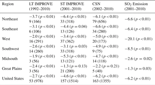
to initial years of network operation can be biased if the num-ber of sites is too few to obtain a representative regional av-erage. We observed this behavior with the regional annual mean IMPROVE data in the early 1990s and in 2000 during network expansion, and we also observed this behavior with CSN data in 2000 and 2001 during the initial years of that network. To avoid these biases, we filtered the regional data to include only data from years with numbers of sites that were within one standard deviation of the average number of sites per year for the entire time period. As a result, the length of the regional trends narrowed relative to the individual site trends shown in Figs. 1 and 3. Long-term (LT) regional IMPROVE trends were computed for 1992–2010 (19 yr); short-term (ST) regional IMPROVE trends were computed for 2001–2010 (10 yr), and CSN trends were computed for 2002–2010 (9 yr). Table 1 lists the number of IMPROVE and CSN sites used in the annual, regional analyses. The number of CSN sites used in the East was greater than IMPROVE sites, and vice versa in the West.
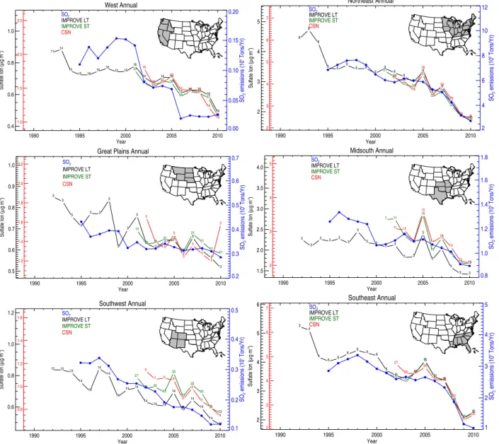
Timelines of annual mean sulfate concentrations and an-nual total CEM SO2 emissions for the contiguous United
States since the early 1990s are shown in Fig. 6. IMPROVE and CSN sulfate concentrations are shown on left axes and SO2 emissions refer to the right axis. CSN and IMPROVE
data are plotted with different scales so that the tracking of the timelines could be more clearly shown. The differ-ence in IMPROVE and CSN data (signified by the shift in scales) should not be interpreted as urban excess, because the large-scale regional analysis includes sites beyond only nearby pairings of urban/rural sites. Also, recall from Fig. 2 that sulfate concentrations are highest in the East where the majority of CSN sites are located. LT IMPROVE data are shown in black, ST IMPROVE data are shown in green, and CSN data are shown in red. The LT and ST IMPROVE data are shown separately because the trends were computed with different numbers of available sites. The number of complete sites with valid data available for a given year is used as the plot symbol for each time series.
The US annual mean sulfate concentrations and SO2
emis-sions have decreased steadily since the mid-1990s. LT IM-PROVE sulfate concentrations decreased in 1992–1993, in-creased in 1997–1998, and inin-creased again in 2005 and 2007 (along with ST IMPROVE and CSN data). Concentrations fell to their lowest values by 2010. In addition, the tracking of the LT IMPROVE, ST IMPROVE, and CSN data from 2000 was quite impressive. The temporal trends in SO2emissions
were similar to sulfate concentrations. The annual mean sul-fate LT IMPROVE trend was−2.7 % yr−1(p <0.01). Since
the early 2000s, ST IMPROVE sulfate decreased at a rate of
−4.6 % yr−1(p <0.01), slightly less than the CSN trend of −6.2 % yr−1(p <0.01). CEM SO2emissions decreased by −6.2 % yr−1(p <0.01) from 2001–2010 (see Table 1).
Table 1.Trends in regional, annual mean IMPROVE and CSN particulate sulfate ion concentrations and annual total power plant (CEM) SO2emissions. The trend (% yr−1)and significance (p) are on top and the number of sites and number of observations (in parentheses) are on the bottom for each region.
Region LT IMPROVE ST IMPROVE CSN SO2Emission
(1992–2010) (2001–2010) (2002–2010) (2001–2010)
Northeast 9 (166)−3.7 (p <0.01) −33 (318)6.4 (p <0.01) 79 (656)−6.1 (p <0.01) −6.6 (p <0.01)
Southeast −3.1 (p <0.01) −4.4 (p=0.04) −6.6 (p <0.01) −6.4 (p <0.01)
6 (106) 13 (126) 34 (280)
West −2.0 (p <0.01) −3.4 (p <0.01) −5.0 (p <0.01) −20.1 (p <0.01)
16 (291) 37 (362) 20 (173)
Southwest −2.6 (p <0.01) −3.1 (p=0.03) −4.9 (p <0.01) −8.5 (p <0.01)
14 (260) 33 (318) 9 (75)
Midsouth −1.9 (p <0.01) −5.3 (p <0.01) −4.7 (p <0.01) −2.6 (p =0.02)
3 (56) 13 (121) 14 (118)
Great Plains −2.4 (p <0.01) −1.3 (p=0.13) −2.2 (p=0.21) −1.3 (p=0.03)
3 (56) 21 (200) 5 (40)
United States −2.7 (p <0.01) −4.6 (p <0.01) −6.2 (p <0.01) −6.2 (p <0.01)
53 (978) 157 (1514) 163 (1355)
U.S. Annual
1990 1995 2000 2005 2010
Year 1.0
1.5 2.0 2.5
Sulfate Ion (
µ
g m
-3) 40 44
46 50 51
51 51 49 50 51
51 51 51
51
50 51
51
51 51
120 137
147 150 149
149 150
150 150
149
129 140
155 159
160 160
154
146 139
SO2 IMPROVE LT
IMPROVE ST
CSN
4 6 8 10 12 14 16 18
SO
2
emissions (10
6 Tons/Yr)
2 3 4 5
Fig. 6.United States annual mean particulate sulfate ion concentra-tions (µg m−3)from long-term (LT) and short-term (ST) IMPROVE
sites (left black axis) and CSN sites (left red axis), and power plant SO2emissions (million t yr−1)(right blue axis). The number of complete sites with valid data available for a given year is used as the plot symbol for each time series.
for each figure. The highest annual total SO2emissions from
power plants in the country were in the upper-right quad-rant of the United States, referred to here as the Northeast-ern region, including the Ohio River valley and Boundary Waters regions and more “traditional” northeastern states. SO2 emissions for this region were nearly double those in
the southeastern United States due to relatively high emis-sions in the Ohio River valley region (see Fig. 5a); however, the 2000–2010 annual emissions decreased at similar rates in the Northeast (−6.6 % yr−1)and Southeast (−6.4 % yr−1)
regions (all regional trends were statistically significant; sig-nificance levels are included in Table 1). SO2emissions in
these regions tracked closely with sulfate concentrations.
SO2emissions in the Midsouth region decreased at a lower
rate (−2.6 % yr−1)and did not track changes in sulfate
con-centrations as closely as the other eastern regions. This may be in part due to the geographic differences in the sites in the Midsouth region. Sulfate concentrations peaked in 2005 at all of the eastern regions and perhaps corresponded to a slight increase in SO2 emissions during that year. SO2emissions
and sulfate concentrations dropped in 2010, with the excep-tion of sulfate concentraexcep-tions in the Southeast region. Note that the temporal behavior of sulfate concentrations and SO2
emissions for the contiguous United States (Fig. 6) were sim-ilar to those at the eastern regions (Fig. 7b, d, f), suggesting that that annual trends for the total United States were be-ing driven by the emissions and concentrations in the eastern United States.
SO2emissions in the West region decreased at the
high-est rate of any region in the United States (−20.1 % yr−1).
Already decreasing SO2 emissions dropped in 2002 due to
the changes at the Centralia Big Hanaford power plant in Washington mentioned earlier and fell again in 2006 due to the closure of the Mohave power plant in Laughlin, Nevada. Emissions in the West after 2006 were the lowest in the coun-try. Decreases in SO2 emissions were flattest in the Great
Plains region (−1.3 % yr−1)compared to the Southwest
re-gion (−8.5 % yr−1). In general, changes in sulfate
concentra-tions at western regions did not track those of SO2emissions
as closely or as strongly as was observed for eastern regions. Recall from Fig. 4b and Sect. 3.2 that since 2000 sulfate concentrations increased in the western United States dur-ing sprdur-ing months, especially in May. A timeline of May monthly mean sulfate concentrations and SO2emissions for
West Annual
1990 1995 2000 2005 2010 Year
0.4 0.6 0.8 1.0
Sulfate Ion (
µ
g m
-3) 11
14
15 15 16 16
16 15 15 16 16 16 16 16
15 16 16 16
16 33 37 37 37 36 36 37 37 37 36 18 20 20 20 20 20 19
18 18 SO2 IMPROVE LT IMPROVE ST CSN 0.00 0.05 0.10 0.15 0.20 SO 2 emissions (10
6 Tons/Yr)
1.0 1.5 2.0 2.5
Northeast Annual
1990 1995 2000 2005 2010
Year 2
3 4 5
Sulfate Ion (
µ g m -3) 8 8 8 9 9 9 9 8 9 9 9 9 9 9 9 9 9 9 9 27 29 32 33 33 33 33 33 33 33 62 66 76 78 79 79 76 72 68 SO2 IMPROVE LT IMPROVE ST CSN 2 4 6 8 10 12 SO 2 emissions (10
6 Tons/Yr)
2 3 4 5 6 7
Great Plains Annual
1990 1995 2000 2005 2010
Year 0.5 0.6 0.7 0.8 0.9 1.0
Sulfate Ion (
µ g m -3) 3 3 3 3 3 3 3 3 3 3 3 3 3 3 3 3 3 3 3 14
19 21 21 21 21 21 21 21 21 5 5 5 5 5 5 5 3 2 SO2 IMPROVE LT IMPROVE ST CSN 0.2 0.3 0.4 0.5 0.6 0.7 SO 2 emissions (10
6 Tons/Yr)
1.2 1.4 1.6 1.8 2.0 2.2 Midsouth Annual
1990 1995 2000 2005 2010
Year 1.5 2.0 2.5 3.0 3.5 4.0
Sulfate Ion (
µ
g m
-3)
3 3
3 3 3 3 3 3 3 3 3 3 3 3 3 3 3 3 3 7 11 13 13 13 13 13 13 13 13 11 13 14 13 14 14 13 13 13 SO2 IMPROVE LT IMPROVE ST CSN 0.8 1.0 1.2 1.4 1.6 1.8 SO 2 emissions (10
6 Tons/Yr)
2 3 4 5
Southwest Annual
1990 1995 2000 2005 2010
Year 0.6
0.8 1.0 1.2
Sulfate Ion (
µ
g m
-3)
12 12 13
14 14 14 14 14 14 14 14 14 14 14 14 14 14 14 14 27 29 32 33 33 33 33 33 33 33 6 7 9 9
9 9 9 9 8 SO2 IMPROVE LT IMPROVE ST CSN 0.1 0.2 0.3 0.4 0.5 SO 2 emissions (10
6 Tons/Yr)
0.8 1.0 1.2 1.4 1.6 Southeast Annual
1990 1995 2000 2005 2010
Year 2 3 4 5 6
Sulfate Ion (
µ g m -3) 3 4 4 6 6
6 6 6 6 6 6 6 6 6 6 6 6 6 6 12 12 12 13 13 13 13 13 13 13 27 29 31 34 33 33 32 31 30 SO2 IMPROVE LT IMPROVE ST CSN 1 2 3 4 5 SO 2 emissions (10
6 Tons/Yr)
2 3 4 5 6 7
Fig. 7.Regional annual mean particulate sulfate ion concentrations (µg m−3)from long-term (LT) and short-term (ST) IMPROVE sites (left
black axis) and CSN sites (left red axis), and power plant SO2emissions (million tons yr−1)(right blue axis) for(a)West(b)Northeast(c)
Great Plains(d)Midsouth(e)Southwest(f)Southeast. The inset maps show the states in the region in gray. The number of complete sites with valid data available for a given year is used as the plot symbol for each time series.
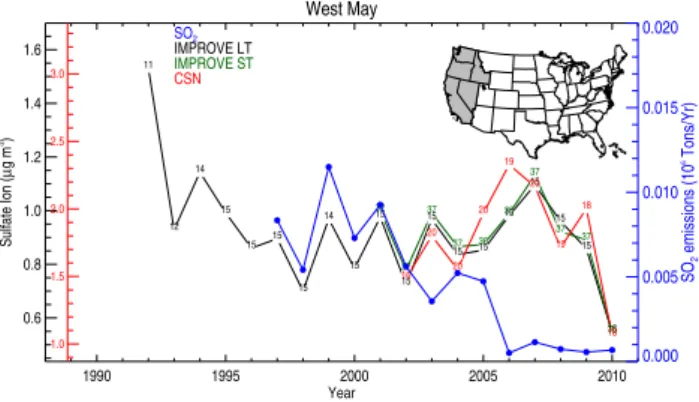
(Fig. 7a), May monthly mean sulfate concentrations steadily increased from early 2000 through 2007, after which they dropped considerably and reached a low value in 2010. The regional pattern demonstrated that this behavior was typical for many urban and rural sites in the West region in spring. Clearly, the May SO2emissions demonstrated very different
behavior. The correlation coefficient for May SO2emissions
and ST rural monthly mean sulfate concentrations in the West wasr=0.09.
As another example of differing behavior between SO2
emissions and sulfate concentrations, recall that winter mean sulfate concentrations increased at a swath of sites stretching
from the northern into the central Great Plains (Fig. 4a), es-pecially in December. A timeline of December monthly, re-gional mean SO2emissions and sulfate concentrations for the
Great Plains region is shown in Fig. 9. Beginning in 2006 re-gional sulfate concentrations rapidly increased through 2010, at rates that reached 17.5 % yr−1(recall the Fort Peck,
Mon-tana, site). In contrast, December regional SO2 emissions
from power plants were flat from 2000 through 2009 and decreased in 2010. The correlation coefficient for December SO2 emissions and ST rural monthly mean sulfate
West May
1990 1995 2000 2005 2010 Year 0.6 0.8 1.0 1.2 1.4 1.6
Sulfate Ion (
µ g m -3) 11 12 14 15 15 15 15 14 15 15 15 15 15 15 15 15 15 15 15 32 37 37 37 36 35 37 37 37 36 16 20 20 20 19 20 19 18 18 SO2 IMPROVE LT IMPROVE ST CSN 0.000 0.005 0.010 0.015 0.020 SO 2 emissions (10
6 Tons/Yr)
1.0 1.5 2.0 2.5 3.0
Fig. 8.May monthly and regional mean particulate sulfate ion con-centrations (µg m−3)for the West region (see gray states on inset
map) from long-term (LT) and short-term (ST) IMPROVE sites (left black axis) and CSN sites (left red axis), and power plant SO2 emis-sions (million t yr−1)(right blue axis). The number of complete
sites with valid data available for a given year is used as the plot symbol for each time series.
Timelines of regional annual mean sulfate concentrations and annual total CEM SO2 emissions tracked closely for
most regions, suggesting a near-linear relationship between average changes in power plant SO2 emissions and sulfate
concentrations. This relationship was evident in the scatter plots of sulfate concentrations and CEM SO2emissions for
regional short-term data shown in Fig. 10a and for NEI total SO2emissions in Fig. 10b. The LT IMPROVE data and the
SO2emissions had a similar relationship. Linear correlation
coefficients were highest for the Northeast and Southeast re-gions where SO2emissions and sulfate concentrations were
largest. It is interesting to note that the apparent response of sulfate to SO2emissions was lower in the Northeast region
relative to the rest of the country. The cause of this is un-known.
4 Discussion and summary
Significant progress has been made in reducing SO2
emis-sions in the United States. The total US SO2emissions (NEI)
have decreased from nearly 31 million tons in 1970 to 8 mil-lion tons in 2010, a nearly four-fold decrease (see Fig. 11). Source categories of the NEI include large electric utili-ties (power plants), industrial, commercial, and institutional sources, including residential heaters and boilers, chemical processes such as chemical production and petroleum refin-ing, on-road vehicles, and non-road vehicles and engines. Since 1975 electric utilities consistently have accounted for roughly two-thirds or greater of total SO2emissions and
re-ductions in power plant emissions primarily accounted for the decrease in total SO2emissions shown in Fig. 11.
How-ever, these SO2 emissions are only from US sources. As
mentioned in Sect. 1, transpacific transport from Asia can influence US sulfate concentrations. Modeling studies such
Great Plains Dec
1990 1995 2000 2005 2010 Year 0.3 0.4 0.5 0.6 0.7 0.8
Sulfate Ion (
µ g m -3) 3 3 3 3 3 3 3 3 3 3 3 3 3 3 3 3 3 3 3 14 21 21 21 21 21 20 21 20 21 5 5 5 5 5 5 4 3 2 SO2 IMPROVE LT IMPROVE ST CSN 0.025 0.030 0.035 0.040 0.045 0.050 0.055 SO 2 emissions (10
6 Tons/Yr)
1.0 1.5 2.0 2.5
Fig. 9.December monthly mean particulate sulfate ion concentra-tions (µg m−3)for the Great Plains region (see gray states on
in-set map) from long-term (LT) and short-term (ST) IMPROVE sites (left black axis) and CSN sites (left red axis), and power plant SO2 emissions (million t yr−1)(right blue axis). The number of
com-plete sites with valid data available for a given year is used as the plot symbol for each time series.
as those performed by Park et al. (2004), Heald et al. (2006), and Chin et al. (2007) implied that SO2emissions from
out-side of the United States can be important contributors to background sulfate concentrations, especially in the West where power plant emissions are low. As SO2emissions in
other countries change, it is possible that transboundary sul-fate contributions could affect US sulsul-fate trends, particularly as SO2emissions in the United States continue to decrease.
Sulfate concentrations decreased significantly at long-term IMPROVE sites in the United States from 1992 to 2010 (−2.7 % yr−1). In 2000 the IMPROVE network expanded
and the CSN came online, nearly tripling the number of sites available for trend analyses. Short-term annual mean urban (2002–2010) and rural (2001–2010) sulfate concentrations decreased by −6.2 % yr−1 and −4.6 % yr−1, respectively,
with stronger rates for regions in the eastern compared to the western United States. Short-term trends in seasonal mean concentrations indicated specific seasons and regions where sulfate concentrations increased. For example, urban and ru-ral mean sulfate concentrations in the western United States in May increased steadily from early 2000 until 2006–2007 after which they dropped (Fig. 8). Additionally, monthly mean maximum sulfate concentrations have shifted from summer to spring for many western sites since 2000 (Hand et al., 2012a). Contributions of sulfate from Asian sources are largest during the spring (Park et al., 2004), and Lu et al. (2011) reported timelines of Chinese SO2emissions that
All Regions Annual
0 1 2 3 4 5 6
SO2 Emissions (10
6
Tons yr-1
) 0
1 2 3 4
Sulfate Concentration (
µ
g m
-3 )
IMPROVE CSN
Northeast r= 0.94,0.91
Southeast r= 0.95,0.97
West r= 0.82,0.74
Southwest r= 0.70,0.90
Midsouth r= 0.76,0.86
Great Plainsr= 0.81,-0.25
United States Annual
0 5 10 15 20
SO2 Emissions (10
6
Tons yr-1
) 0
1 2 3 4
Sulfate Concentration (
µ
g m
-3 )
IMPROVE CSN
CEM CEM NEI
NEI r= 0.94,r= 0.94,r= 0.94,r= 0.94, 0.94 0.94 0.93 0.93
Fig. 10. (a)Regional annual mean short-term particulate sulfate ion concentration (µg m−3)from IMPROVE and CSN versus
an-nual total power plant SO2emissions (million t yr−1)from con-tinuous emission monitoring (CEM) power plants.(b)US annual mean short-term sulfate ion concentration (µg m−3)for IMPROVE
and CSN versus annual total SO2 emissions (million tons yr−1) from continuous emission monitoring (CEM) power plants and the National Emission Inventory (NEI). Correlation coefficients (r) are listed in blue for IMPROVE and red for CSN and are 99 % confident for values above 0.77 (IMPROVE) and 0.80 (CSN).
in 2006 concentrations increased rapidly and reached their highest values in 2010 (see Fig. 9). Hand et al. (2012b) spec-ulated several possible causes, such as impacts from oil and gas development, transport from oil sand regions in Canada, meteorological influences, or a likely combination of all. In both the spring and winter cases, the known local and
re-United States Annual SO2
1970 1980 1990 2000 2010
Year 0
5 10 15 20 25 30
SO
2
emissions (10
6 Tons/Yr)
NEI Total
NEI Electric Utilities CEM Power Plants
Fig. 11.US annual SO2emissions (million t yr−1)from the
Na-tional Emission Inventory (NEI) total sources, NEI electric utility sources, and continuous emission monitoring (CEM) power plant sources.
gional SO2emissions could not account for the sulfate
con-centration behavior.
The Regional Haze Rule (RHR) sets as the natural back-ground goal aerosol concentrations corresponding to no US anthropogenic sources. RHR background levels of sulfate ion concentrations are 0.17 µg m−3in the East and 0.09 µg m−3
in the West (U.S. EPA, 2003). As shown in Fig. 10a for all re-gions, as the US power plant SO2emissions approached zero,
the sulfate concentrations did not. This offset is indicative of contributions from non-power-plant SO2 emissions and
non-US sources. The NEI SO2emissions, available only for
the entire United States, included non-power plant emissions but did not account for natural sources (with the exception of a very small fire contribution). Therefore the intercept of the regression between sulfate concentrations and NEI SO2
emissions provides an estimate of background sulfate due to natural sources, non-regulated sources, and international an-thropogenic contributions (see Fig. 10b). Using Theil regres-sion, the background sulfate concentrations for the United States were 0.39 ± 0.12 µg m−3 and 0.66 ± 0.24 µg m−3 for
ST IMPROVE and CSN data, respectively. These values are larger than the RHR natural background estimates but are in line with those of Park et al. (2004), who estimated background sulfate ion concentrations of 0.31 µg m−3 and
0.28 µg m−3 for the western and eastern United States,
re-spectively.
The results presented here imply that on an annual basis, the strategies for reducing SO2emissions from power plants
ramifications for sulfate’s role in visibility degradation, cli-mate forcing, and health effects. However, this analysis also revealed that for certain regions and seasons, factors other than known local and regional power plant emissions have had significant impacts on sulfate concentrations. In general, the linear relationship between SO2 emissions and sulfate
concentrations in the western United States was not as ro-bust as seen in the East. Understanding the sources of these increased concentrations has important implications for our current approach for air pollution mitigation strategies, as they appear to be insufficient for some seasons and regions.
Supplementary material related to this article is
available online at: http://www.atmos-chem-phys.net/12/ 10353/2012/acp-12-10353-2012-supplement.pdf.
Acknowledgements. This work was funded by the National Park
Service under contract H2370094000. The assumptions, findings, conclusions, judgments, and views presented herein are those of the authors and should not be interpreted as necessarily representing the National Park Service policies.
Edited by: R. Cohen
References
Blanchard, C. L., Hidy, G. M., Tanenbaum, S., Edgerton, E. S., and Hartsell, B. E.: The Southeastern Aerosol Research and Charac-terization (SEARCH) Study: Temporal trends in gas and PM con-centrations, 1999–2010, J. Air Waste Manage., in press, 2012. Chin, Mian, Diehl, T., Ginoux, P., and Malm, W.: Intercontinental
transport of pollution and dust aerosols: implications for regional air quality, Atmos. Chem. Phys., 7, 5501–5517, doi:10.5194/acp-7-5501-2007, 2007.
Eldred, R.: Sulfur-Sulfate History for IMPROVE, IMPROVE Data advisory, http://vista.cira.colostate.edu/improve/Publications/ GrayLit/006 Sulfur-Sulfate History/006 sulfur-sulfate history. htm (last access: 1 July 2012), 2001.
Gebhart, K. A., Schichtel, B. A., Barna, M. G., and Malm, W. C.: Quantitative back-trajectory apportionment of sources of partic-ulate sulfate at Big Bend National Park, TX, Atmos. Environ., 40, 2823–2834, 2006.
Hand, J. L., Copeland, S. A., Day, D. E., Dillner, A. M., Idresand, H., Malm, W. C., McDade, C. E., Moore, Jr., C. T., Pitchford, M. L., Schichtel, B. A., and Watson, J. G.: IM-PROVE (Interagency Monitoring of Protected Visual Environ-ments): Spatial and seasonal patterns and temporal variabil-ity of haze and its constituents in the United States: Report V, CIRA Report ISSN: 0737-5352-87, http://vista.cira.colostate. edu/improve/Publications/Reports/2011/2011.htm (last access: 1 July 2012), 2011.
Hand, J. L., Schichtel, B. A., Pitchford, M., Malm, W. C., and Frank, N. H.: Seasonal composition of remote and urban fine particu-late matter in the United States, J. Geophys. Res., 117, D05209, doi:10.1029/2011JD017122, 2012a.
Hand, J. L., Gebhart, K. A., Schichtel, B. A., and Malm, W. C.: Increasing trends in wintertime particulate sulfate and nitrate ion concentrations in the Great Plains of the United States (2000– 2010), Atmos. Environ., 55, 107–110, 2012b.
Heald, C. L., Jacob, D. J., Park, R. J., Alexander, B., Fairlie, T. D., Yantosca, R. M., and Chu, D. A.: Transpacific transport of Asian anthropogenic aerosols and its impact on surface air quality in the United States, J. Geophys. Res., 111, D14310, doi:;10.1029/2005JD006847, 2006.
Hidy, G. M., Mueller, P. K., and Tong, E. Y.: Spatial and tempo-ral distributions of airborne sulfate in parts of the United States, Atmos. Environ., 12, 735–752, 1978.
Husain, L., Dutkiewicz, V. A., and Das, M.: Evidence for decrease in atmospheric sulfur burden in the eastern United States caused by reduction in SO2emissions, Geophys. Res. Lett., 25, 967– 970, 1998.
Husain, L., Parekh, P. P., Dutkiewicz, V., Khan, A. R., Yang, K., and Swami, K.: Long-term trends in atmospheric con-centrations of sulfate, total sulfur, and trace elements in the northeastern United States, J. Geophys. Res., 109, D18305, doi:10.1029/2004JD004877, 2004.
Hyslop, N. P. and White, W. H.: An evaluation of interagency mon-itoring of protected visual environments (IMPROVE) collocated precision and uncertainty estimates, Atmos. Environ., 42, 2691– 2705, 2008.
Hyslop, N. P., Trzepla, K., and White, W. H.: Reanalysis, with con-sistent analytical protocol, of archived IMPROVE PM2.5 sam-ples previously collected, analyzed, and reported over a 15-year period, Environ. Sci. Technol., 46, 10106–10113, 2012. Kiehl, J. T., and Briegleb, B. P.: The relative roles of sulfate aerosols
and greenhouse gases in climate forcing, Science, 260, 311–314, 1993.
Jaffe, D., Tamura, S., and Harris, J.: Seasonal cycle and composi-tion of background fine particles along the west coast of the US, Atmos. Environ, 39, 297–306, 2005.
Lehmann, C. M. B. and Gay, D. A.: Monitoring long-term trends of acidic wet deposition in US precipitation: Results from the National Atmospheric Deposition Program, Power Plant Chem., 13, 386–393, 2011.
Lin, M., Fiore, A. M., Horowitz, L. W., Cooper, O. R., Naik, V., Holloway, J., Johnson, B. J., Middlebrook, A. M., Oltmans, S. J., Pollack, I. B., Ryerson, T. B., Warner, J. X., Wiedeninmyer, C., Wilson, J., and Wyman, B.: Transport of Asian ozone pollution into surface air over the western United States in spring, J. Geo-phys. Res., 117, D00V07, doi:10.1029/2011JD016961, 2012. Lu, Z., Zhang, Q., and Streets, D. G.: Sulfur dioxide and primary
carbonaceous aerosol emissions in China and India, 1996–2010, Atmos. Chem. Phys., 11, 9839–9864, doi:10.5194/acp-11-9839-2011, 2011.
Malm, W. C.: Characteristics and origins of haze in the continental United States, Earth-Sci. Rev., 33, 1–36, 1992.
Malm, W. C., Sisler, J. F., Huffman, D., Eldred, R. A., and Cahill, T. A.: Spatial and seasonal trends in particle concentration and op-tical extinction in the United States, J. Geophys. Res., 99, 1347– 1370, 1994.
Murphy, D. M., Chow, J. C., Leibensperger, E. M., Malm, W. C., Pitchford, M., Schichtel, B. A., Watson, J. G., and White, W. H.: Decreases in elemental carbon and fine particle mass in the United States, Atmos. Chem. Phys., 11, 4679–4686, doi:10.5194/acp-11-4679-2011, 2011.
Park, R. J., Jacob, D. J., Field, B. D., Yantosca, R. M., and Chin, M.: Natural and transboundary pollution influ-ences on sulfate-nitrate-ammonium aerosols in the United States: Implications for policy, J. Geophys. Res., 109, D15204, doi:10.1029/2003JD004473, 2004.
Peltier, R. E., Hecobian, A. H., Weber, R. J., Stohl, A., Atlas, E. L., Riemer, D. D., Blake, D. R., Apel, E., Campos, T., and Karl, T.: Investigating the sources and atmospheric processing of fine particles from Asia and the Northwestern United States mea-sured during INTEX B, Atmos. Chem. Phys., 8, 1835–1853, doi:10.5194/acp-8-1835-2008, 2008.
Petters, M. D., Carrico, C. M., Kreidenweis, S. M., Prenni, A. J., Demott, P. J., Collett Jr., J. L., and Moosm¨uller, H.: Cloud con-densation nucleation activity of biomass burning aerosol, J. Geo-phys. Res. 114, D22205, doi:10.1029/2009JD012353, 2009. Rohr, A. C. and Wyzga, R. E.: Attributing health effects to
indi-vidual particulate matter constituents, Atmos. Environ., 62, 130– 152, 2012.
Schichtel, B. A., Pitchford, M. L., and White, W. H.: Comments on “Impact of California’s Air Pollution Laws on Black Carbon and their Implications for Direct Radiative Forcing” by R. Bahadur et al., Atmos. Environ., 45, 4116–4118, 2011.
Tai, A. P. K., Mickley, L. J., and Jacob, D. J.: Correlations between fine particulate matter (PM2.5) and meteorological variables in the United States: Implications for the sensitivity of PM2.5 to climate change, Atmos. Environ., 44, 3976–3984, 2010. Tai, A. P. K., Mickley, L. J., Jacob, D. J., Leibensperger, E. M.,
Zhang, L., Fisher, J. A., and Pye, H. O. T.: Meteorological modes of variability for fine particulate matter (PM2.5) air quality in the United States: implications for PM2.5sensitivity to climate change, Atmos. Chem. Phys., 12, 3131–3145, doi:10.5194/acp-12-3131-2012, 2012.
Theil, H.: A rank-invariant method of linear and polynomial regres-sion analysis, Proc. Kon. Ned. Akad. V. Wetensch. A, 53, 386– 392, 521–525, 1397–1412, 1950.
U.S. Environmental Protection Agency: Regional Haze Regula-tions; Final Rule, 40 CFR 51, Federal Register, 64, 35714– 35774, 1999.
U.S. Environmental Protection Agency: Guidance for estimat-ing natural visibility conditions under the Regional Haze Pro-gram, Contract No. 68-D-02-0261, Work Order No. 1-06, http:// www.epa.gov/ttn/oarpg/t1/memoranda/rh envcurhr gd.pdf (last access: 1 July 2012), 2003.
U.S. Environmental Protection Agency: Program back-ground, PM2.5Spec. Network Newsl., 1, http://www.epa.gov/ttn/amtic/ files/ambient/pm25/spec/spnews1.pdf (last access: 1 July 2012), 2004.
U.S. Environmental Protection Agency: Technology Transfer Net-work Clearinghouse for Inventories and Emission Factors, Na-tional Emissions Inventory (NEI) air pollutant emissions trends data, http://www.epa.gov/ttnchie1/trends (last access: 12 Decem-ber 2011), 2011a.
U.S. Environmental Protection Agency: Air Markets Program Data, available at http://ampd.epa.gov/ampd (last access: 8 November 2011), 2011b.
White, W. H.: Inconstant bias in XRF sulfur- Advisory Update to da0012, Doc #da0023, http://vista.cira.colostate.edu/improve/ Data/QA QC/Advisory/da0023/da0023 DA SSO4 update.pdf (last access: 1 July 2012), 2009.
White, W. H., Ashbaugh, L. L., Hyslop, N. P., and McDade, C. E.: Estimating measurement uncertainty in an ambient sulfate trend, Atmos. Environ., 39, 6857–6867, 2005.
Van Curen, R. A. and Cahill, T. A.: Asian aerosols in North Amer-ica: Frequency and concentration of fine dust, J. Geophys. Res., 107, 4804, doi:10.1029/2002JD002204, 2002.