Modelled and observed changes in aerosols and surface solar radiation over Europe between 1960 and 2009

(1)

ACPD

15, 13457–13513, 2015

Modelled and observed changes in

European aerosols 1960–2009

S. T. Turnock et al.

Title Page

Abstract Introduction

Conclusions References

Tables Figures

◭ ◮

Back Close

Full Screen / Esc

Printer-friendly Version Interactive Discussion

Discussion

P

a

per

|

Discussion

P

a

per

|

Discussion

P

a

per

|

Discussion

P

a

per

|

Atmos. Chem. Phys. Discuss., 15, 13457–13513, 2015 www.atmos-chem-phys-discuss.net/15/13457/2015/ doi:10.5194/acpd-15-13457-2015

This discussion paper is/has been under review for the journal Atmospheric Chemistry and Physics (ACP). Please refer to the corresponding final paper in ACP if available.

Modelled and observed changes in

aerosols and surface solar radiation over

Europe between 1960 and 2009

S. T. Turnock1, D. V. Spracklen1, K. S. Carslaw1, G. W. Mann1,2,

M. T. Woodhouse1,*, P. M. Forster1, J. Haywood3, C. E. Johnson3, M. Dalvi3,

N. Bellouin4, and A. Sanchez-Lorenzo5

1

Institute of Climate and Atmospheric Science, School of Earth and Environment, University of Leeds, Leeds, UK

2

National Centre for Atmospheric Science, University of Leeds, Leeds, UK

3

Met Office, Fitzroy Road, Exeter, Devon, UK

4

Department of Meteorology, University of Reading, Reading, UK

5

Pyrenean Institute of Ecology, Spanish National Research Council, Zaragoza, Spain

*

now at: CSIRO Ocean and Atmosphere, Aspendale, Victoria, Australia Received: 2 April 2015 – Accepted: 20 April 2015 – Published: 8 May 2015 Correspondence to: S. T. Turnock (s.t.turnock12@leeds.ac.uk)

(2)

ACPD

15, 13457–13513, 2015

Title Page

Tables Figures

◭ ◮

Back Close

Full Screen / Esc

Discussion

P

a

per

|

Discussion

P

a

per

|

Discussion

P

a

per

|

Discussion

P

a

per

|

Abstract

Substantial changes in anthropogenic aerosols and precursor gas emissions have oc-curred over recent decades due to the implementation of air pollution control legisla-tion and economic growth. The response of atmospheric aerosols to these changes and the impact on climate are poorly constrained, particularly in studies using detailed 5

aerosol chemistry climate models. Here we compare the HadGEM3-UKCA coupled chemistry-climate model for the period 1960 to 2009 against extensive ground based observations of sulfate aerosol mass (1978–2009), total suspended particle matter

(SPM, 1978–1998), PM₁₀ (1997–2009), aerosol optical depth (AOD, 2000–2009) and

surface solar radiation (SSR, 1960–2009) over Europe. The model underestimates 10

observed sulfate aerosol mass (normalised mean bias factor (NMBF)₌−0.4), SPM

(NMBF=−0.9), PM₁₀(NMBF=−0.2) and aerosol optical depth (AOD, NMBF=−0.01)

but slightly overpredicts SSR (NMBF=0.02). Trends in aerosol over the observational

period are well simulated by the model, with observed (simulated) changes in sulfate

of−68 % (−78 %), SPM of−42 % (−20 %), PM₁₀ of−9 % (−8 %) and AOD of −11 %

15

(−14 %). Discrepancies in the magnitude of simulated aerosol mass do not affect the

ability of the model to reproduce the observed SSR trends. The positive change in ob-served European SSR (5 %) during 1990–2009 (“brightening”) is better reproduced by

the model when aerosol radiative effects (ARE) are included (3 %), compared to

simu-lations where ARE are excluded (0.2 %). The simulated top-of-the-atmosphere aerosol 20

radiative forcing over Europe under all-sky conditions increased by 3 W m−2during the

period 1970–2009 in response to changes in anthropogenic emissions and aerosol concentrations.

1 Introduction

Aerosols can cause acid deposition, degradation of atmospheric visibility, changes to 25

(3)

ACPD

15, 13457–13513, 2015

Title Page

Tables Figures

◭ ◮

Back Close

Full Screen / Esc

Discussion

P

a

per

|

Discussion

P

a

per

|

Discussion

P

a

per

|

Discussion

P

a

per

|

human health. Aerosols interact with climate by absorbing and reflecting incoming solar

radiation and by modifying the microphysical properties of clouds. These e_ffects have

been defined in the latest Intergovernmental Panel on Climate Change (IPCC) report (Boucher et al., 2013) as aerosol–radiation interactions (ARI) and aerosol-cloud inter-actions (ACI). Aerosols (also referred to as Particulate Matter (PM)) are detrimental to 5

air quality and human health, as particles below a certain size can penetrate into the lungs causing respiratory and cardiovascular problems (COMEAP, 2010). Strategies that attempt to mitigate climate change and poor air quality are inherently connected and have the potential to induce both benefits and penalties for either depending on the particular species targeted (Arneth et al., 2009; Ramanathan and Feng, 2009; Fiore 10

et al., 2012).

Here we use a global coupled chemistry-climate model to improve our understanding of changes in aerosols over Europe from 1960 to 2009. The climate impact of aerosols over this period, in response to emission changes, was calculated as an aerosol

ra-diative forcing. An assessment of the confidence in this e_ffect was obtained from the

15

ability of the model to reproduce observed long term changes in a number of aerosol properties including mass concentrations and aerosol optical depth.

Anthropogenic emissions of aerosol particles and their precursors have increased

significantly since pre-industrial times. For example, global SO₂ emissions have

in-creased by a factor of 60 from the pre-industrial to a peak in the 1970s (Lamarque 20

et al., 2010; Granier et al., 2011; Smith et al., 2011). However, from the 1980s onwards regional reductions in anthropogenic emissions (mainly North America and Europe) have occurred due to air quality mitigation strategies, which has led to a decline in

Eu-ropean SO₂ emissions of 73 % between 1980 and 2004 (Vestreng et al., 2007; Hand

et al., 2012). European emissions of other anthropogenic species such as oxides of 25

nitrogen (NO_x), carbon monoxide (CO) and black carbon (BC) have also decreased

(4)

ACPD

15, 13457–13513, 2015

Title Page

Tables Figures

◭ ◮

Back Close

Full Screen / Esc

Discussion

P

a

per

|

Discussion

P

a

per

|

Discussion

P

a

per

|

Discussion

P

a

per

|

leading to an increase in SO₂ emissions of a factor of seven from the 1960s to the

present day (Smith et al., 2011).

Changes in anthropogenic emissions and aerosol concentrations affect the Earth’s

climate (Arneth et al., 2009; Ramanathan and Feng, 2009; Fiore et al., 2012). The

e_ffect of past and future changes in emissions on aerosols and their associated climate

5

impacts is uncertain (Penner et al., 2010; Chalmers et al., 2012). In addition, emission inventories of aerosols and their precursor species account for large uncertainty in models (de Meij et al., 2006). It is therefore important to understand and evaluate the changes to aerosol processes and properties that have occurred over recent decades where we have aerosol measurements.

10

Ground-based monitoring networks providing observations of aerosol concentrations and physio-chemical properties were established following air pollution control legisla-tion. The longest continuous measurements of aerosols are available in North Amer-ica and Europe from the 1970s to present day. In Europe, observations of aerosol mass concentrations (both sulfate and total) are available from the European Monitor-15

ing and Evaluation Programme (EMEP) network (Tørseth et al., 2012) and similar data for North America are available from the Integrated Monitoring of Protected Visual En-vironments (IMPROVE) network (http://vista.cira.colostate.edu/improve/). In addition, Aerosol Optical Depth (AOD) has been monitored in Europe over the last decade by the ground-based Aerosol Robotic Network (AERONET) (Holben et al., 1998). There 20

are limitations in the spatial and temporal extent of the data from these networks, as well as the consistency of the instrumental techniques used and components mea-sured throughout the monitoring period. However they do provide a useful source of multi decadal aerosol data with which to evaluate model predictions.

Several studies have analysed long-term trends in observed aerosols. Tørseth et al. 25

(2012) used observations from the EMEP network to show a decline in sulfate aerosol

mass from the 1970s to present day and a decline in PM₁₀ (mass of particles of

di-ameter<10 µm) from 2000 to 2009. Asmi et al. (2013) and Barmpadimos et al. (2012)

(5)

ACPD

15, 13457–13513, 2015

Title Page

Tables Figures

◭ ◮

Back Close

Full Screen / Esc

Discussion

P

a

per

|

Discussion

P

a

per

|

Discussion

P

a

per

|

Discussion

P

a

per

|

to 15 years across Europe. However, Collaud Coen et al. (2013) found no significant changes in aerosol optical properties over Europe for a similar period. Similarly Harri-son et al. (2008) analysed changes in aerosol mass concentrations over the UK and reported relatively stable concentrations over 2000 to 2010, even when emission re-ductions are anticipated to have occurred.

5

Evaluating the ability of chemistry-climate models to reproduce observed trends is

necessary in order to reliably predict the climate effects of aerosols over this period.

Many studies qualitatively match the direction of observed trends in aerosol but under-estimate both absolute concentrations and the magnitude of observed trends (Berglen et al., 2007; Colette et al., 2011; Koch et al., 2011; Chin et al., 2014). Leibensperger 10

et al. (2012) used the Chemical Transport Model (CTM) GEOS-Chem to evaluate aerosol trends over the USA at decadal time slices and found that sulfate but not BC was represented well by the model. A multi-model assessment of aerosol trends in Europe over the last decade showed models successfully simulate observed negative

trends in PM₁₀ but fail to reproduce the positive trends observed at some locations

15

and typically underestimate absolute concentrations (Colette et al., 2011). Observed reductions in sulfate over Europe have also been underestimated by other studies (Berglen et al., 2007; Koch et al., 2011). Over Europe, Skeie et al. (2011) reproduced the observed change in decadal average sulfate concentrations but overestimated ni-trate aerosol concentrations.

20

Several studies (Lamarque et al., 2010; Shindell et al., 2013) have also assessed long term changes in AOD. Lamarque et al. (2010) evaluated simulations of present day AOD against AERONET observations and reported a relatively good reproduction of inter-annual variability, except in regions of high AOD. Shindell et al. (2013) assessed AOD from the models involved in the Atmospheric Chemistry and Climate Model Inter 25

(6)

ACPD

15, 13457–13513, 2015

Title Page

Tables Figures

◭ ◮

Back Close

Full Screen / Esc

Discussion

P

a

per

|

Discussion

P

a

per

|

Discussion

P

a

per

|

Discussion

P

a

per

|

Changes in surface solar radiation (SSR) do not provide a direct measurement of aerosols but they can be used to infer their influence on the surface radiation balance. The Global Energy Balance Archive (GEBA) provides long term observations of SSR from the 1950s until present day over a large part of Europe (Sanchez-Lorenzo et al., 2013). These measurements can also be used as a general measure to validate ra-5

diation balance predictions from global climate models against the observed surface variations. Such observations have shown that the European “dimming” period of the 1980s and the subsequent “brightening” period of the 1990s–2000s can be attributed

partly to changes in clouds, concentrations of aerosols and aerosol-cloud effects (Wild,

2009). Model simulations have been evaluated against SSR observations and demon-10

strated issues in simulating the timing and magnitude of observed SSR trends. In an as-sessment of the models contributing to the 5th Coupled Model Intercomparison Project (CMIP5), Allen et al. (2013) showed that the dimming trend over Europe was

under-estimated in all models, potentially due to an under-represented aerosol direct e_ffect.

However, the CMIP5 models were able to reproduce the observed brightening trend. 15

Folini and Wild (2011) performed transient simulations with ECHAM5-HAM over Eu-rope (with interactive aerosols) and found that simulated reductions in SSR occurred too early in the model whereas, the increase in SSR was correctly timed. Using a re-gional climate model over Europe driven by reanalysis data, Chiacchio et al. (2015) overestimated SSR, simulated a premature onset of dimming and demonstrated that 20

only simulations including aerosols were able to reproduce the observed brightening trend. In addition, Koch et al. (2011) simulated the correct inter-decadal variability in SSR but underestimated the magnitude of observed SSR.

These previous studies have either simplified their treatment of aerosols or the model was evaluated against a limited range of aerosol properties over a relatively coarse 25

(7)

ACPD

15, 13457–13513, 2015

Title Page

Tables Figures

◭ ◮

Back Close

Full Screen / Esc

Discussion

P

a

per

|

Discussion

P

a

per

|

Discussion

P

a

per

|

Discussion

P

a

per

|

climate model, which includes aerosol microphysics (aerosol number and mass size distributions). We evaluate the ability of the model to consistently capture observed changes in bulk in situ aerosol properties (PM and chemical components) as well as radiative properties (AOD, SSR) over Europe. We also calculate the regional top of atmosphere radiative perturbations due to simulated changes in aerosols. This has 5

enabled a detailed regional analysis and evaluation of the changing radiative impact of aerosols due to variations in emissions.

Section 2 describes the HadGEM3-UKCA model, the simulations performed and the long term observations used. Section 3 discusses and evaluates the simulated changes to European aerosols and surface solar radiation. Section 4 presents aerosol 10

radiative forcing over Europe. Conclusions are presented in Sect. 5.

2 Methods

2.1 Model description and simulations

2.1.1 General

We used the coupled chemistry-climate model HadGEM3-UKCA to study the inter-15

action between chemistry, aerosols and the impacts on the radiation balance of the

climate system. HadGEM3-UKCA is part of the third generation of the Met Office’s

Hadley Centre Global Environment Model (HadGEM) family, which incorporates an on-line treatment of chemistry and aerosols through the United Kingdom Chemistry and

Aerosols (UKCA) programme. The Met Office Unified Model (UM) acts as the

dynami-20

(8)

ACPD

15, 13457–13513, 2015

Title Page

Tables Figures

◭ ◮

Back Close

Full Screen / Esc

Discussion

P

a

per

|

Discussion

P

a

per

|

Discussion

P

a

per

|

Discussion

P

a

per

|

Morgenstern et al. (2009) and O’Connor et al. (2014) describe the incorporation and evaluation of UKCA into HadGEM.

HadGEM3-UKCA is used here in atmosphere-only mode. We output monthly 3-D

aerosol and radiation fields for the years 1960–2009 at a resolution of 1.875◦×1.25◦

(approximately 140 km at mid latitudes) with 63 vertical levels up to 40 km. The 3-D 5

meteorological fields were nudged at 6 hourly intervals to the European Centre for Medium-Range Weather Forecasts (ECMWF) Reanalysis (ERA-40) (Uppala et al., 2005) for the years 1960 to 2000 and ERA-Interim (Dee et al., 2011) for 2000 to 2009. Sea surface temperatures and sea ice fields were prescribed in accordance with those used in CMIP5 (Hurrell et al., 2008). Coupling between the land surface and atmo-10

sphere was simulated using the Met O_ffice Surface Exchange Scheme (MOSES;

Es-sery et al., 2002). By nudging to re-analysis data, we ensure that the meteorological conditions in the model match those under which aerosol observations were taken.

Tropospheric ozone-HO_x-NO_x-VOC chemistry was calculated using the mechanism

described by O’Connor et al. (2014), which includes reactions of odd oxygen (O_x),

nitro-15

gen (NO_Y), hydrogen (HO_x=OH+HO₂) and CO, as well as methane and other short

chain non-methane volatile organic compounds (VOCs). The scheme has been ex-tended to include additional sulfur (Mann et al., 2010), monoterpene (Spracklen et al., 2006) and isoprene (Scott et al., 2014) chemistry.

The Fast-J photolysis scheme is implemented within UKCA to calculate online pho-20

tolysis rates based on the distribution of clouds, ozone and aerosols (Wild et al., 2000). Dry and wet deposition of gas phase species is described in O’Connor et al. (2014).

HadGEM3-UKCA uses the modal aerosol scheme of the Global Model of Aerosol Processes (GLOMAP-mode) (Mann et al., 2010). GLOMAP-mode uses log-normal modes to represent the aerosol size distribution and simulates the evolution of the size-25

resolved number and mass of aerosol particles with di_fferent compositions. GLOMAP

(9)

ACPD

15, 13457–13513, 2015

Title Page

Tables Figures

◭ ◮

Back Close

Full Screen / Esc

Discussion

P

a

per

|

Discussion

P

a

per

|

Discussion

P

a

per

|

Discussion

P

a

per

|

aerosols in the nucleation (diameterD <10 nm), Aitken (D=10–100 nm),

accumula-tion (D=100 nm–1 µm) and coarse (D >1 µm) modes. In this study the model is set

up to simulate sulfate, BC, organic carbon (OC) and sea salt aerosol in 5 different

modes (4 soluble and 1 insoluble Aitken modes). Secondary organic aerosol (SOA) is formed from products of monoterpene oxidation, which are generated at 13 % yield 5

and assumed to be involatile (Spracklen et al., 2006). There is no representation of ammonium nitrate in this version of the model. Mineral dust is simulated using a sepa-rate 6-bin scheme developed by Woodward (2001) and covers particle sizes from 0.03 to 30 µm in radius.

2.1.2 Aerosol radiative effects

10

The Edwards–Slingo radiation code (Edwards and Slingo, 1996) calculates changes in the Earth’s radiation balance from chemical and aerosol species. ARI (aerosol

direct effects) are calculated according to Bellouin et al. (2013) from

waveband-averaged scattering and absorption coefficients obtained from modelled size

distri-butions and a volume-weighted average of component refractive indices within each 15

mode. GLOMAP-mode provides the aerosol fields for the calculation of ACI on-line within the model, in accordance with that described in Bellouin et al. (2013). Simulated cloud condensation nuclei (CCN) concentrations are used to calculate cloud droplet number (CDN) concentrations based on the empirical relationship derived by Jones

et al. (2001). The cloud albedo effect is calculated using simulated CDN. The coupling

20

of UKCA to the precipitation scheme potentially allows for the e_ffect of aerosols on

cloud lifetime (rapid adjustments fro ACI) to be diagnosed. This can be done by

calcu-lating the influence they have on CDN concentrations, cloud effective radius and

ulti-mately the auto-conversion of cloud drops to precipitation, as described in Jones et al. (2001). However, in this study, because we nudge to reanalysis fields, the changes in 25

(10)

ACPD

15, 13457–13513, 2015

Title Page

Tables Figures

◭ ◮

Back Close

Full Screen / Esc

Discussion

P

a

per

|

Discussion

P

a

per

|

Discussion

P

a

per

|

Discussion

P

a

per

|

The radiation scheme was called twice each time step (every 30 min) in a double-call radiation configuration (Bellouin et al., 2013). The first call uses the modelled aerosol fields and the second call uses an aerosol-free atmosphere for the clear-sky radiative calculation and a prescribed default CDN field (based on an aerosol climatology) for the cloud radiation calculation. This approach therefore eliminates the model’s radiatively-5

driven response to changes in aerosols, enabling the radiative forcing from ARI and

ACI to be calculated with no rapid adjustments to clouds permitted from either effect.

Here we calculate an aerosol radiative forcing (only from the direct and first indirect

effects) as the difference between monthly values in each year of the simulation and

the monthly mean aerosol radiative state in the period 1980–2000. 10

2.1.3 Aerosol emissions

Sea salt emissions are calculated using the surface wind speed and the parameteri-sation of Gong (2003). Emissions from tropospheric volcanoes (both continuous and time-averaged sporadic) are included from Andres and Kasgnoc (1998) and Halmer et al. (2002) using the AEROCOM recommendations. Dimethyl sulfide (DMS) emis-15

sions are calculated from monthly sea-water concentration fields (Kettle and Andreae, 2000) and a wind speed dependent air–sea exchange parameterisation (Liss and Mer-livat, 1986). Wildfires (biomass burning) emissions are from the MACCity inventory (Granier et al., 2011) for 1980 to 2009 and from the RETRO inventory from 1960 to 1980 (Schultz et al., 2008). Monoterpene emissions from vegetation are prescribed as 20

monthly mean fields from Guenther et al. (1995). Dust emissions from the surface are calculated on-line using a 6-bin scheme (Woodward, 2001) and depend on the particle size distribution of the soil, surface soil type (represented by a bare soil fraction), soil moisture and wind speed. Dust is emitted when the wind speed exceeds a threshold value and if the soil moisture is below a certain level.

25

Monthly mean anthropogenic emissions of CO, SO₂, NO_x, OC and BC from 1960–

2009 are taken from the MACCity inventory (Granier et al., 2011). Emissions are

(11)

ACPD

15, 13457–13513, 2015

Title Page

Tables Figures

◭ ◮

Back Close

Full Screen / Esc

Discussion

P

a

per

|

Discussion

P

a

per

|

Discussion

P

a

per

|

Discussion

P

a

per

|

Reference Concentration Pathway (RCP) scenario 8.5 for energy, transportation, in-dustry, shipping, agriculture, residential and waste sectors.

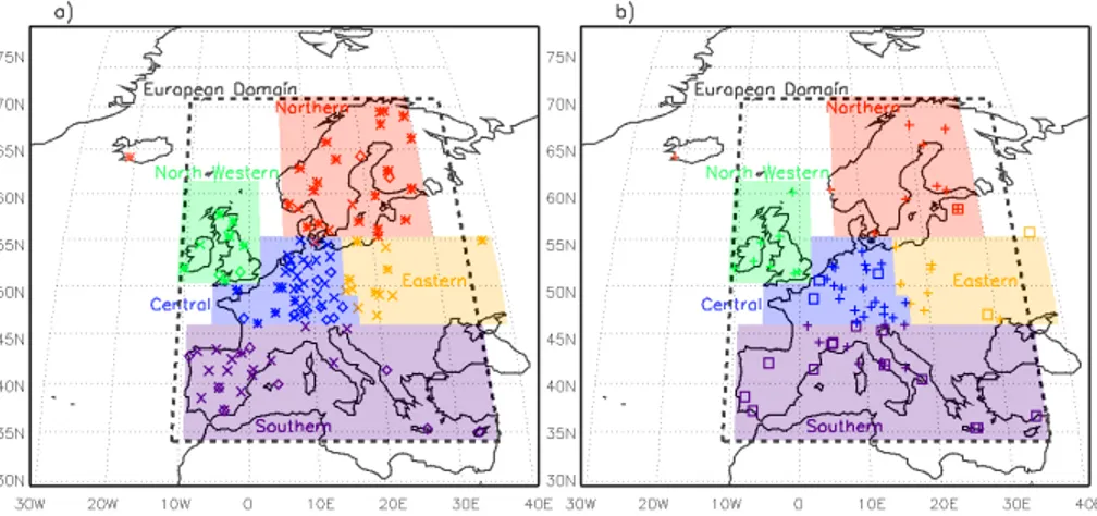
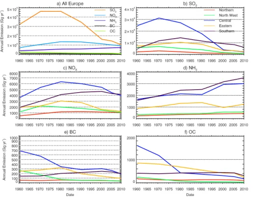
Figure 1 shows the European and regional domains used throughout this study.

Fig-ure 2 shows the emissions of SO₂, OC, BC, NH₃ and NO_x across Europe from the

MACCity inventory between 1960 and 2009. Anthropogenic emissions of SO₂over the

5

European domain have increased from 33 Tg yr−1 in 1960 to apeak of 46 Tg yr−1 in

1980 before decreasing at a relatively constant rate to 11 Tg yr−1in 2009 (Fig. 2a).

Be-tween 1980 and 2009, European anthropogenic SO₂emissions in this dataset declined

by 70 %, in agreement with previous assessments (Vestreng et al., 2007; Tørseth et al.,

2012). The emissions of NO_xhave decreased by 20 % and followed a similar temporal

10

trend to SO₂. A continuous decline in BC and OC emissions occurred from the 1960s

to present day, due to reductions in the residential sector, partially o_ffset by recent

in-creases from the transportation sector. The emissions of NH₃across Europe (not used

in this study) increased continuously over the period 1960–2009, driven largely by the agriculture sector.

15

Figure 2b–f shows the annual emissions of each species from the MACCity inventory

across the individual European regions. Emissions of OC (Fig. 2f) and SO₂ (Fig. 2b)

have decreased across all the di_fferent European regions. Emissions of NO_x and BC

(Fig. 2c and e) increase until the 1980s–1990s before declining across all regions, except in southern Europe. Anthropogenic emissions from northern and central Europe 20

have declined from the 1980s onwards, whereas emissions from southern Europe have either increased or remained unchanged.

2.2 Observations

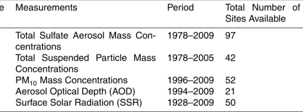
Ground-based measurements of aerosols used in this study are listed in Table 1 and include aerosol mass concentrations (sulfate and total mass) from the EMEP network 25

(12)

loca-ACPD

15, 13457–13513, 2015

Title Page

Tables Figures

◭ ◮

Back Close

Full Screen / Esc

Discussion

P

a

per

|

Discussion

P

a

per

|

Discussion

P

a

per

|

Discussion

P

a

per

|

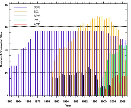
tion of all the measurement sites along with the 5 regions of Europe. Figure 3 shows the temporal evolution in the number of measurement sites used in this analysis for each observation. We note that the number of locations reporting sulfate and SSR has declined since 2000.

2.2.1 EMEP observations

5

The EMEP network has reported the concentrations of sulfate and total aerosol mass at locations across Europe from 1978 until present day (Tørseth et al., 2012). Mea-surements of total Suspended Particle Matter (SPM) are an early measure of particu-late matter and available from 1978 to 2005, with most measurements from Germany, Switzerland and Spain. However, only measurements up to and including 1998 are 10

used due to the reduced availability of data in the period 1999–2005 (Fig. 3). The SPM measurements cover all particle sizes and may be influenced by local sources of very

large particles (diameter>10 µm). Measurements of PM₁₀ are available from EMEP

from 1996 until present day. Sulfate aerosol mass measurements are available from 1978 until present day.

15

We used sulfate aerosol mass, PM₁₀ and total SPM from the sites that have been

continuously operating for more than 5 years (Fig. 1a). The measurements were made

using di_fferent measurement techniques and time frequencies (hourly and daily). The

raw data were screened to remove any anomalous data points according to the flag in the original data records. Monthly and annual mean values were then calculated from 20

the screened data for sites that had more than 75 % of measurements in the averaging period.

2.2.2 AOD

The AERONET program is a ground-based network of sun photometers, currently with more than 200 sites providing aerosol optical, microphysical and radiative properties 25

(13)

mid-ACPD

15, 13457–13513, 2015

Title Page

Tables Figures

◭ ◮

Back Close

Full Screen / Esc

Discussion

P

a

per

|

Discussion

P

a

per

|

Discussion

P

a

per

|

Discussion

P

a

per

|

1990s but most sites only started operating within the last ten years (Fig. 3) and there are relatively few consistent long term datasets available before 2000. We used the Level 2.0 data product (cloud-screened and quality assured) from 20 sites that have been operating for longer than 5 years over Europe between 2000 and 2009. AOD measurements have the best record for wavelengths of 440, 500 and 675 nm. We used 5

the 440 nm wavelength as it has the best spatial and temporal coverage.

2.2.3 Surface solar radiation

GEBA contains worldwide measurements of energy fluxes at the surface from more than 2000 sites, with the highest density over Europe. Monthly mean values of

inci-dent SSR (expressed as mean irradiance, in W m−2) have been obtained from 56 sites

10

across Europe starting before the 1970s, provided by Sanchez-Lorenzo et al. (2013), and including more than 20 sites that have data in the 1960s. The length of this obser-vational record enabled the model evaluation to be extended prior to the availability of sulfate data. These measurements therefore enable an indirect evaluation of aerosol changes in the model across the entire time period of the simulations and also valida-15

tion of how changes in aerosols can affect the Earth’s radiation balance.

2.3 Model evaluation metrics

Comparisons were made using monthly and annual mean values at individual moni-toring locations and also across Europe as a whole. Model values were interpolated to each measurement site. The absolute and percentage change in the simulated and ob-20

served values of sulfate, SPM, PM₁₀, AOD and SSR were calculated as the difference

between the mean of the initial 5 years and most recent 5 years of data.

The temporal trend in simulated and observed data was calculated by fitting an ordi-nary least squares linear model to the data using the function below:

Y_i =a+bX_i(i =1,. . .,n) (1)

(14)

ACPD

15, 13457–13513, 2015

Title Page

Tables Figures

◭ ◮

Back Close

Full Screen / Esc

Discussion

P

a

per

|

Discussion

P

a

per

|

Discussion

P

a

per

|

Discussion

P

a

per

|

The standard error (SE) of the trend line was used to provide an assessment of the

error. For each simulated and observed trend,±two SE in the gradient was applied to

provide an uncertainty range. Firstly the SD of the residuals (σ) was determined and

then used to calculate the SE.

The simulated temporal trends were evaluated by comparing against observed 5

trends; if the gradient of the simulated and observed trends are within ± two SE of

each other we considered them to be similar.

An assessment of model accuracy is provided here by calculating the normalised mean bias factor (NMBF) of the model when compared to the observations (Yu et al., 2006). This metric is symmetric (i.e. not biased towards under prediction or over pre-10

diction) and is not biased when a low number of observed values are used. It is defined as:

NMBF₌S[exp(|ln(M/O)|)−1], (2)

Where

S=(M−O)/|M−O|. (3)

15

whereM represents the model values andOrepresents the observed values. The sign

of the NMBF indicates whether the model underestimates (negative) or overestimates (positive) the observed values. For a negative NMBF, the model values are a factor

of (1−NMBF) below the observed values and for a positive NMBF the model values

are a factor of (1+NMBF) above the observations (Yu et al., 2006). That is, NMBF=

20

−0.5 means the model is a factor 1.5 low biased and NMBF₌0.5 means the model is

a factor 1.5 high biased.

The goodness of fit between the model and observations is obtained by calculating

the square of the linear Pearson correlation coe_fficient. A measure of the di_fference

between model and observational values is provided by calculating the Root Mean 25

(15)

ACPD

15, 13457–13513, 2015

Title Page

Tables Figures

◭ ◮

Back Close

Full Screen / Esc

Discussion

P

a

per

|

Discussion

P

a

per

|

Discussion

P

a

per

|

Discussion

P

a

per

|

3 Results

3.1 Simulated European aerosols and surface solar radiation 1960 to 2009

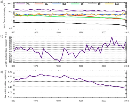
Figure 4a shows the simulated European (land only) mass concentrations of the

dif-ferent aerosol components over the period 1960–2009. Simulated PM₁₀ declines from

the early 1980s until 2009, coinciding with the reduction in anthropogenic emissions 5

(Fig. 2). Continually decreasing mass concentrations of BC and OC are simulated be-tween 1960 and 2009. Simulated sulfate mass concentrations increase from 1960 to a peak around 1980 and decrease thereafter.

Figure 4b shows that simulated European SSR decreases from 1960 to 1980 (“dim-ming”), then increases until 2009 (“brightening”). Simulated European AOD (Fig. 4c) 10

increases from 1960 to a peak in 1973 before decreasing till 2009 to an AOD that is lower than that simulated 1960.

3.2 Model evaluation

3.2.1 Sulfate aerosol mass

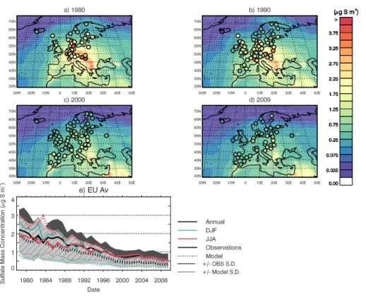
Figure 5a–d compares simulated annual mean sulfate concentrations over Europe in 15

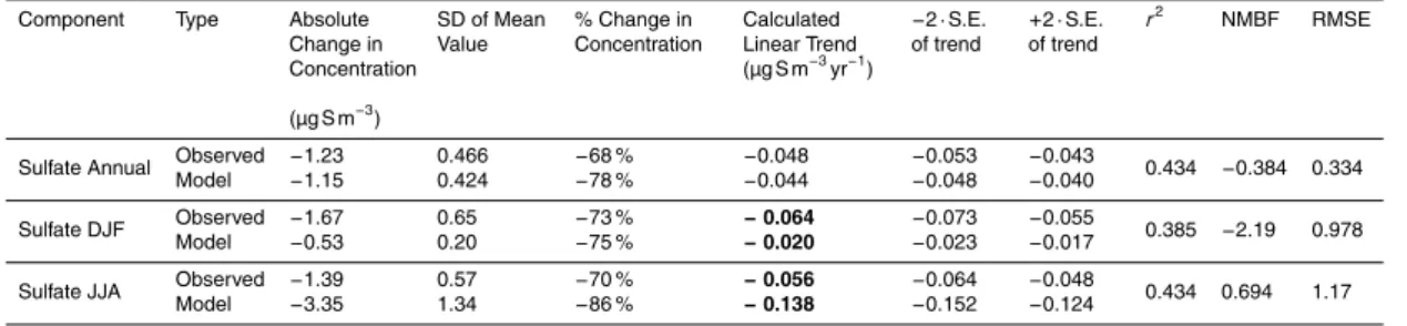
1980, 1990, 2000 and 2009 against observations. Observed and simulated annual mean European sulfate aerosol concentrations declined by 68 and 78 % respectively over the period 1978–2009 (Table 2). In 1980 (Fig. 5a) simulated and observed sul-fate concentrations were largest in central Europe. In 2000 and 2009 (Fig. 5c and d) both simulated and observed sulfate concentrations in Central Europe have declined 20

substantially, with the largest simulated concentrations over south east Europe. The model underestimates European annual mean sulfate aerosol mass

concentra-tions in the period 1978–2009 (NMBF=−0.384, Table 2), with summertime

concentra-tions slightly overestimated (NMBF=0.694) and wintertime concentrations

underesti-mated (NMBF₌−2.19). Figure 6 shows the range of model bias in seasonal sulfate

(16)

ACPD

15, 13457–13513, 2015

Title Page

Tables Figures

◭ ◮

Back Close

Full Screen / Esc

Discussion

P

a

per

|

Discussion

P

a

per

|

Discussion

P

a

per

|

Discussion

P

a

per

|

across European regions for the period 1978–2009. In summer, the model underesti-mates observed sulfate across northern and southern Europe (NMBF between 0 and

−1), and overestimates sulfate in central and eastern Europe (NMBF<1). The model

consistently underestimates wintertime sulfate (NMBF of−1 to−6) across all the

Eu-ropean regions, with the largest discrepancy occurring in northern Europe. 5

An underprediction of wintertime European sulfate concentrations has been previ-ously reported and may be due to an underestimation of oxidants in the model (Berglen et al., 2007; Manktelow et al., 2007; Langmann et al., 2008). In wintertime over

north-ern Europe, the region with largest model bias, low concentrations of H₂O₂ limit

in-cloud aqueous phase oxidation of SO₂. Under these conditions oxidation by ozone is

10

the dominant sulfate formation mechanism (Kreidenweis, 2003). We hypothesise that oxidation by ozone could be under-represented in the model, resulting in an underesti-mation of wintertime sulfate. This will be explored further in a future publication. Model underestimation could also be due to an artificially high wet deposition rate of sulfate, caused by an enhanced occurrence of drizzle precipitation within this version of the 15

model (Walters et al., 2011).

Although the model underestimates absolute sulfate concentrations, the simulated

trend over the period 1978–2009 (−0.04±0.002 µg S m−3yr−1) is in good agreement

with the observed trend (−0.05±0.002 µg S m−3yr−1), at least on a European-wide

annual mean basis (Fig. 5e). These trends can be considered similar as they are 20

within two standard errors of each other. The largest decline in both simulated and observed sulfate concentrations occurred during 1980–2000, when average

concen-trations changed by−0.05 µg S m−3yr−1. Between 1980 and 2000, average simulated

and observed concentrations declined by 50–60 %, corresponding with a 60–70 %

decrease in anthropogenic emissions of SO₂ (Fig. 2). A smaller reduction in sulfate

25

aerosol mass of 13–18 % was simulated and observed in the period 2000–2009, when

average concentrations changed by−0.015 µg S m−3yr−1. Figure 7 compares the

(17)

concen-ACPD

15, 13457–13513, 2015

Title Page

Tables Figures

◭ ◮

Back Close

Full Screen / Esc

Discussion

P

a

per

|

Discussion

P

a

per

|

Discussion

P

a

per

|

Discussion

P

a

per

|

trations. However, linear trends in wintertime sulfate aerosol mass are underestimated (by a factor of 3) but overestimated in summertime (by a factor of 1.3). This corre-sponds with the calculated NMBFs for winter and summertime mass concentrations, which showed an under and over prediction respectively.

3.2.2 Total aerosol mass

5

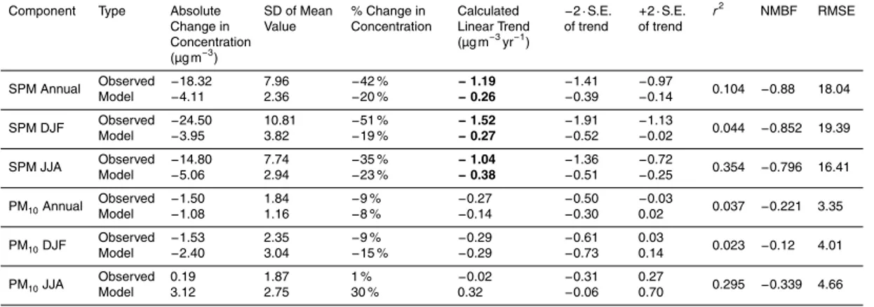
Figure 8a and b compares simulated and observed annual mean total SPM concentra-tions over Europe in 1980 and 1990. The spatial changes in SPM over this period are less distinct than that for sulfate. Simulated and observed SPM decreases over cen-tral Europe and increases over eastern Europe between 1980 and 1990. In contrast to sulfate aerosol mass, the simulated 20 % decrease in SPM mass concentrations in the 10

period 1978–1998 is considerably lower than the 50 % observed decrease.

The model underpredicts the observed European annual mean SPM mass

concen-trations, with a NMBF of−0.88 in the period 1978–1998 (Table 3). A consistent

under-prediction of observed SPM concentrations was modelled across all European regions in both summer and winter (Fig. 9a). The model substantially underpredicts SPM con-15

centrations in wintertime for southern and eastern Europe (NMBF of−8 to−0.5). In

summertime and across all European regions the model underpredicts observations by

a smaller amount (NMBF of 0 to−2). The large underprediction of observed SPM mass

concentrations could indicate that an additional emission source or process for gener-ating supermicron aerosol mass is missing from the model, particular in the 1980s and 20

early 1990s when the model bias is largest.

Figure 8c shows that the larger observed trend in European annual mean SPM mass

over the period 1978–1998 of−1.19±0.22 µg m−3yr−1 is substantially different to the

simulated trend of −0.26±0.12 µg m−3yr−1 (Table 3). Figure 10a shows that the

ob-served trends in SPM mass concentrations are underpredicted at all the measurement 25

locations, with little seasonal differences. The calculated trends in simulated and

ob-served SPM values are considered to be di_fferent as they are outside the range of±

(18)

ACPD

15, 13457–13513, 2015

Title Page

Tables Figures

◭ ◮

Back Close

Full Screen / Esc

Discussion

P

a

per

|

Discussion

P

a

per

|

Discussion

P

a

per

|

Discussion

P

a

per

|

Figure 8d and e compares simulated and observed annual mean PM₁₀ mass

con-centrations over Europe in 2000 and 2009. A slight reduction in PM₁₀ mass

concen-trations of 8–9 % was both observed and simulated over this period (Table 3), with the largest reductions occurring over central and north-eastern continental Europe.

The model generally underestimates observed PM₁₀mass concentrations (NMBF of

5

0 to−1) for the majority of European regions and across most of the evaluated years

(Fig. 9b). An exception occurs across northern and north-western Europe in winter-time where the model overpredicts concentrations (NMBF of 0 to 2). This is potentially caused by an overestimation of sea salt aerosol (as also seen in studies by Mann et al.,

2010, 2012), so mostly affects coastal locations. Overall the model simulates European

10

PM₁₀ mass concentrations between 1997 and 2009 within a factor of 2 and is much

improved when compared to the simulation of total SPM between 1978 and 1998.

The temporal changes in PM₁₀ mass concentrations (Fig. 8f) highlight the smaller

difference between simulated and observed PM₁₀ across Europe compared to SPM.

The linear trends for observed (−0.27±0.24 µg m−3yr−1) and simulated (−0.14±

15

0.16 µg m−3yr−1) PM₁₀ mass concentrations over the period 1997–2009 are similar

(gradients within twice the standard error of each other) (Table 3). However, Fig. 10b shows that the magnitude of the observed downward trends is slightly underpredicted

at the majority of measurement locations, with little difference between summer and

winter. 20

The model underpredicts SPM mass concentrations by up to 20 µg m−3in the 1980s

and PM₁₀ by less than 5 µg m−3in the 2000s. This larger underprediction in the 1980s

could be due to errors in the measurement of SPM, as most of these observations are not well documented (Tørseth et al., 2012) and may have substantial uncertainty.

We compared SPM and PM₁₀ observations during a period when both variables were

25

observed at 6 monitoring sites in Spain, and found SPM was greater than PM₁₀ by

6–17 µg m−3. Taking this into account, along with the better model agreement for PM₁₀

(19)

ACPD

15, 13457–13513, 2015

Title Page

Tables Figures

◭ ◮

Back Close

Full Screen / Esc

Discussion

P

a

per

|

Discussion

P

a

per

|

Discussion

P

a

per

|

Discussion

P

a

per

|

model. Potential anthropogenic sources of coarse particles that are not represented in

the model include road tra_ffic dust and construction sources.

Underprediction of aerosol mass could be due to underestimation of aerosol sources, as well as missing aerosol sources from the model. The model does not include nitrate

aerosol which could account for 1–3 µg m−3of aerosol mass over Europe (Fagerli and

5

Aas, 2008; Bellouin et al., 2011; Pozzer et al., 2012). The reductions in SO₂emissions

and increase in NH₃emissions across Europe over the last 30 years (Fig. 2) could have

important impacts on aerosol composition (Fagerli and Aas, 2008). In historical periods

with high SO₂ emissions, sulfate aerosol will dominate and nitrate concentrations are

likely to be small. In the recent past and future, declines in SO₂ and sulfate aerosol

10

mass, coupled with an increase in NH₃emissions may lead to increased nitrate aerosol

concentrations. The model also does not include primary biological aerosol sources,

which may contribute 1–2 µg m−3 to PM₁₀ mass over Europe (Heald and Spracklen,

2009); the contribution toD >10 µm is not known.

Uncertainty in aerosol precursor emissions will also contribute to the model-15

observation discrepancy. In particular, domestic wood burning and wild fires could contribute up to 50 % of OC locally over Europe and may be underestimated in emis-sion datasets (Hodzic et al., 2007; Langmann et al., 2008; Manders et al., 2012). The calculation of SOA is also a large uncertainty, particularly the proportions from an-thropogenic and biogenic sources. Global aerosol models typically underpredict the 20

amount of organic aerosols in the atmosphere (Tsigaridis et al., 2014), particularly from anthropogenic sources (Volkamer et al., 2006; Farina et al., 2010; Spracklen et al., 2011). Anthropogenic sources (or anthropogenically modified biogenic sources)

that are not accounted for here may contribute up to 3 µg m−3 of SOA over Europe

(Spracklen et al., 2011). 25

(20)

ACPD

15, 13457–13513, 2015

Title Page

Tables Figures

◭ ◮

Back Close

Full Screen / Esc

Discussion

P

a

per

|

Discussion

P

a

per

|

Discussion

P

a

per

|

Discussion

P

a

per

|

3.2.3 Aerosol optical depth

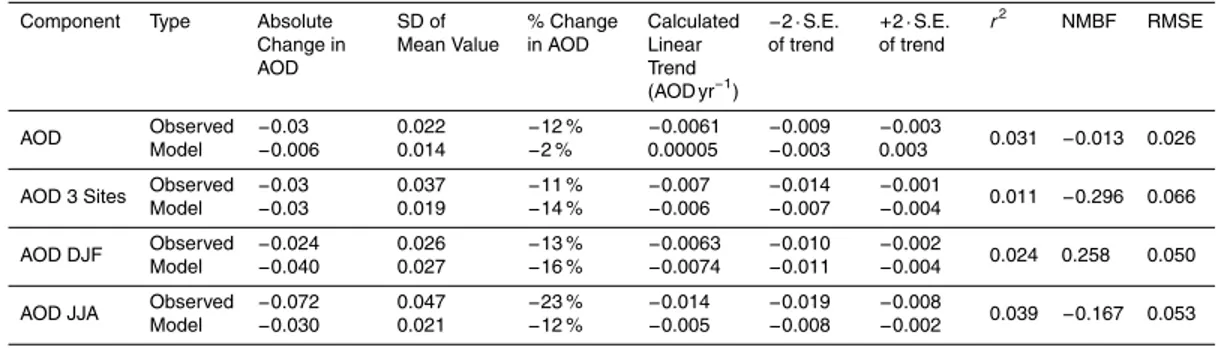
Figure 11a and b compares simulated and observed annual mean AOD at 440 nm in 2000 and 2009. The largest simulated and observed AOD occurs over eastern and south-eastern Europe. The model is relatively unbiased against annual mean AOD

(NMBF₌−0.013). The model captures the observed seasonal cycle in European AOD

5

with highest AOD in the summer and lowest in the winter, but overestimates wintertime

AOD (NMBF=0.258) and underestimates summertime AOD (NMBF=−0.167)

(Ta-ble 4). These seasonal biases are of opposite sign to those for sulfate and PM₁₀.

How-ever, we note that simulation of AOD requires information on aerosol optics, aerosol

size distribution and atmospheric humidity meaning it is difficult to relate to

compar-10

isons of surface aerosol mass.

Observed and simulated AOD has declined over the period 2000 to 2009 (Fig. 11c). Table 4 shows that at the three monitoring locations with the longest data records (9– 10 years), simulated and observed AOD has declined by a similar magnitude (11–14 %)

but AOD is underestimated by the model (NMBF=−0.296). The observed AOD trend

15

at the three long term sites in the period 2000–2009 is−0.007±0.004 yr−1and is similar

to that modelled of −0.006±0.0008 yr−1 (Table 4). The trend in observed wintertime

AOD (−0.006±0.002 yr−1) is well captured by the model (−0.007±0.002 yr−1). The

larger observed summertime trend of−0.014±0.003 yr−1is underestimated (−0.005±

0.002 yr−1). The ability of the model to reproduce the decline in AOD is similar to that

20

for sulfate and PM₁₀.

3.2.4 Surface solar radiation

Figure 12 shows simulated and observed annual mean SSR anomalies across Europe between 1960 and 2009, relative to a 1980–2000 mean. The long term mean was based on the period 1980–2000, considered to be the period with the most reliable 25

(21)

ACPD

15, 13457–13513, 2015

Title Page

Tables Figures

◭ ◮

Back Close

Full Screen / Esc

Discussion

P

a

per

|

Discussion

P

a

per

|

Discussion

P

a

per

|

Discussion

P

a

per

|

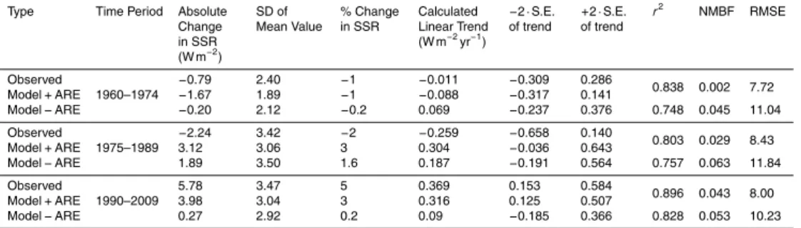
values (Table 5). The observed SSR anomaly is generally positive and relatively con-stant in the period 1960–1974. There is a decrease in observed SSR from 1975 until the late 1980s, after which a strong increase in SSR is observed from 1990 to 2009.

Between 1990 and 2009 both the observed and simulated European SSR

in-creases by 5.8 and 4.0 W m−2 respectively, with similar positive linear trends (0.37 to

5

0.32 W m−2yr−1 – Table 5). The highest spatial correlation (r2=0.90) between

mod-elled and observed SSR values occurs in the period 1990–2009, whereas the bias

(NMBF₌0.04) and error (RMSE₌8.0) in SSR are similar to that in 1975–1989. The

positive SSR trend (“brightening”) observed between the late 1980s and 2009 is re-produced by the model, but simulated brightening begins several years earlier than 10

observed. The positive trend in SSR anomaly across Europe from the mid-1980s to present day corresponds with the observed and simulated decrease in aerosol con-centrations. Figure 12 also shows the modelled all-sky SSR anomalies without aerosol

radiative e_ffects (ARE). Without ARE the simulated trend in SSR is underestimated

(0.09±0.14 W m−2yr−1), suggesting that changes in aerosol concentrations are a

dom-15

inant driver of SSR trends during this period. The simulated positive trend in SSR in-cluding ARE presented here is in agreement with other studies over this period (Wild, 2009; Allen et al., 2013; Sanchez-Lorenzo et al., 2013; Chiacchio et al., 2015).

In the period 1975–1989 both the modelled and observed SSR anomalies are gen-erally negative, which coincides with the maximum anthropogenic emissions and at-20

mospheric aerosol loading. Over this period the observed SSR decreases by an

av-erage of 2.2 W m−2, whilst simulated SSR increases by 3.1 W m−2 (Table 5). A similar

discrepancy in sign and magnitude is also apparent in the linear trends of the model

(0.30±0.17 W m−2yr−1) and observations (−0.26±0.20 W m−2yr−1). This reflects the

models inability to simulate the timing and magnitude of the observed dimming trend in 25

SSR values between 1975 and 1989 (Fig. 12). Over this period the simulated and

ob-served SSR values have a lower correlation (r2=0.80) and larger error (RMSE₌8.43)

(22)

indi-ACPD

15, 13457–13513, 2015

Title Page

Tables Figures

◭ ◮

Back Close

Full Screen / Esc

Discussion

P

a

per

|

Discussion

P

a

per

|

Discussion

P

a

per

|

Discussion

P

a

per

|

cating that errors in the simulation of aerosol are not causing simulated discrepancy in SSR during this period.

Over the period 1960–1974 simulated European annual mean SSR remained rel-atively constant (Fig. 12) and is of a similar magnitude (Table 5) to that observed. Over this period the observed SSR anomalies are positive (compared to a 1980–2000 5

mean), whilst the modelled SSR anomalies are negative. The small observed trend

of−0.01±0.15 W m−2yr−1over the period 1960–1974 is overestimated by the model

(−0.09±0.11 W m−2yr−1). The stronger simulated negative trend in SSR between 1960

and 1974 indicates that the dimming observed in the period 1974–1989 occurs too early in the model. The model without ARE does not show a dimming trend over this 10

period (but does have a large uncertainty, Table 5), which implies that the discrepancy in the SSR trend could be due to uncertainties in simulated aerosols.

Understanding the discrepancy in simulated SSR prior to 1980 is difficult because

aerosol observations are not available. Possible causes of model discrepancy include errors in simulated aerosol, problems with the observations, or the ECMWF reanalysis 15

product. With regards to observational uncertainties, there were fewer observations of SSR before 1970 (Fig. 3) and there is also a larger correction factor associated with data from the available sites (Sanchez-Lorenzo et al., 2013). This suggests that obser-vational error may be larger in the early period. Prior to 2000, the model is forced by the ERA-40 reanalysis. ERA-40 was improved in the 1970s by the inclusion of additional 20

measurements, most notably from satellites (Uppala et al., 2005). Larger errors in the reanalyses prior to 1980 (Uppala et al., 2005) could cause errors in the generation of

clouds by the host GCM, which would a_ffect simulated SSR.

3.2.5 Evaluation summary

Figure 13 summarises the comparison between simulated and observed sulfate, SPM, 25

PM₁₀, AOD and SSR across Europe, separately for their entire operational period

and also for the period 2000–2009 (when PM₁₀ and AOD observations are

(23)

pe-ACPD

15, 13457–13513, 2015

Title Page

Tables Figures

◭ ◮

Back Close

Full Screen / Esc

Discussion

P

a

per

|

Discussion

P

a

per

|

Discussion

P

a

per

|

Discussion

P

a

per

|

riods. The largest under prediction occurs for SPM (1978–1998, NMBF=−0.88), with

smaller underpredictions for sulfate (1978–2009, NMBF₌−0.38) and PM₁₀ (1997–

2009, NMBF=−0.22). Simulated European annual mean SSR has a smaller model

bias (1960–2009, NMBF = 0.02). Over the period 2000–2009, the model has

com-paratively small biases in AOD (NMBF₌−0.013) and SSR (NMBF₌0.036) but larger

5

biases for sulfate (NMBF=−0.71) and PM₁₀ (NMBF=−0.22). Underestimation of

sur-face sulfate and PM₁₀ is therefore not manifested in the simulation of AOD or SSR.

Calculation of AOD requires information on the aerosol vertical profile, aerosol optics, aerosol size distribution and atmospheric humidity. Simulation of SSR strongly depends on model representation of clouds. A direct comparison of model performance in sim-10

ulating surface aerosol mass with AOD or SSR is therefore complicated. Figure 14 shows the spatial correlation and variability (represented by the SD in observed values

normalised to the modelled values, SD_obs/SD_mod) in sulfate, SPM, PM₁₀, AOD and

SSR. In general SSR and sulfate are better simulated in terms of spatial correlation

and variability, with poorer model simulation of SPM, PM₁₀and AOD.

15

The observed negative trends in sulfate, PM₁₀ and AOD (−0.05 µg S m−3yr−1,

−0.27 µg m−3yr−1 and −0.007 yr−1) are all well reproduced by the model

(−0.04 µg S m−3yr−1, −0.14 µg m−3yr−1 and −0.006 yr−1). Over the period 1990 to

2009, observed trends in SSR (0.37 W m−2yr−1) are also well simulated by the model

when ARE are included (0.32 W m−2yr−1), but poorly simulated when ARE are

ex-20

cluded (0.09 W m−2yr−1). This confirms that being able to simulate the decline in

aerosol concentrations over Europe is important for reproducing the observed bright-ening trend in SSR between 1990 and 2009. Prior to 1990, the model does not simulate trends in SSR as well, but few aerosol observations are available to determine the rea-son for model failure, which could be caused by issues with simulated aerosol, clouds 25

(24)

ACPD

15, 13457–13513, 2015

Title Page

Tables Figures

◭ ◮

Back Close

Full Screen / Esc

Discussion

P

a

per

|

Discussion

P

a

per

|

Discussion

P

a

per

|

Discussion

P

a

per

|

4 European aerosol radiative forcing trends

Figure 15 shows the changes in simulated European mean top of atmosphere (TOA) outgoing shortwave radiation, relative to a 1980 to 2000 mean, under all-sky (a) and

clear-sky conditions (b). Here we define this di_fference in TOA shortwave radiation

as a radiative forcing (RF) between the current year and the long term mean state. 5

European mean all-sky RF (Fig. 15a) decreases by 2.0 W m−2 (cooling trend) over

the period 1960–1972, corresponding with the increase in simulated aerosol loading.

From 1973 to 2009, European mean all-sky radiation increases by 3.0 W m−2(warming

trend), corresponding to the simulated reduction of aerosols. All-sky RF showed the

largest increase of 6.0 W m−2 over central Europe between 1973 and 2009, which is

10

consistent with this region having experienced the largest change in anthropogenic emissions (Fig. 2) and aerosol concentrations (Fig. 8). Other regions of Europe have a similar temporal change but with a smaller magnitude.

The simulated clear-sky aerosol TOA RF (Fig. 15b) is similar to that simulated

un-der all-sky conditions. European mean clear-sky RF decreased by 1.5 W m−2between

15

1960 and 1972 (cooling) and from 1973 to 2009 it increased by 3.0 W m−2

(warm-ing). Marmer et al. (2007) reported a similar change of₊2.0 W m−2in the direct

short-wave RF from sulfate aerosols over Europe between 1980 and 2000. This indicates the strong influence directly exerted by aerosols on the European radiative balance in response to changes in anthropogenic emissions. An estimate of the cloud albedo 20

effect is obtained as the difference between the all-sky and clear-sky RF. Over the

pe-riod 1973–2009 the cloud albedo effect is estimated to have increased by 0.44 W m−2

(warming), indicating that is is a relatively small change when compared to that from

the direct effect.

The changes in aerosol RF we simulate over Europe are slightly larger than those 25

calculated for the USA by Leibensperger et al. (2012) of approximately ₊1 W m−2 for

the direct effect and +1 W m−2 for the indirect (first and second) effects. The smaller

(25)

ACPD

15, 13457–13513, 2015

Title Page

Tables Figures

◭ ◮

Back Close

Full Screen / Esc

Discussion

P

a

per

|

Discussion

P

a

per

|

Discussion

P

a

per

|

Discussion

P

a

per

|

the smaller reductions in sulfate aerosol mass concentrations observed over the USA (40 %), when compared to that observed over Europe (70 %).

The calculated changes in all-sky TOA RF indicate the extent to which changes in

anthropogenic emissions over the last 50 years have affected the European radiative

balance. Reductions in anthropogenic aerosols have resulted in a positive response 5

in the European radiative balance. We estimate that the magnitude of these emission

reductions has caused European mean all-sky RF to increase by 3.0 W m−2 between

the mid-1970s and 2009, mainly due to the direct aerosol e_ffect (as shown by similar

changes in the clear-sky RF). The agreement between the model and observations in the changes in aerosols and in the brightening period of the surface radiation bal-10

ance between the 1990 and 2009 provides confidence in the magnitude and temporal change of the simulated TOA RF over this period when most of the change occurs

(2.0 W m−2). Future work needs to explore the potential climate implications from these

changes to the radiative balance. It will be important to understand the role of Euro-pean air quality legislation in observed emission reductions as this may have important 15

implications when considering the impact of future air quality mitigation measures on climate.

5 Conclusions

We used the HadGEM3-UKCA coupled chemistry climate model to simulate changes in aerosols between 1960 and 2009, a period over which anthropogenic sources of 20

aerosol have changed substantially. We evaluated the model against European

obser-vations of sulfate aerosol mass, total suspended particulate matter (SPM), PM₁₀mass

concentrations, aerosol optical depth (AOD) and surface solar radiation (SSR). We also calculated the impact of changes in atmospheric aerosols on European aerosol radiative forcing.

25

The model underpredicts sulfate aerosol mass concentrations (NMBF₌−0.4), SPM

(26)

ACPD

15, 13457–13513, 2015

Title Page

Tables Figures

◭ ◮

Back Close

Full Screen / Esc

Discussion

P

a

per

|

Discussion

P

a

per

|

Discussion

P

a

per

|

Discussion

P

a

per

|

aerosol mass could be due to uncertainties in the observations (Tørseth et al., 2012), an overestimation of deposition processes or underestimated sources of PM including nitrate, anthropogenic SOA, domestic biomass combustion, dust and primary

biolog-ical aerosol particles. The larger underestimation of particles with diameter>10 µm

suggests that the sources of such particles may be more uncertain and are not well 5

treated by the model. The model particularly underestimates sulfate in winter and over northern Europe potentially due to an under-representation of the in-cloud oxidation of sulfur species to sulfate via reaction with ozone or an enhanced wet deposition rate, caused by artificially high drizzle precipitation. Bias in simulated AOD (2000–

2009, NMBF=−0.01) are smaller than for surface aerosol concentrations. Calculation

10

of AOD requires information on the aerosol vertical profile, aerosol optics, aerosol size distribution and atmospheric humidity and complicates any direct comparison between surface aerosol mass and AOD.

Observed trends in surface aerosol mass and AOD were generally well represented by the model. Sulfate aerosol mass declines by 68–78 % in both the observations and 15

model between 1978 and 2009, consistent with the decrease in SO₂ emissions over

Europe. The observed European annual mean SPM decreased by 42 % between 1978 and 1998, compared to a simulated decrease of 20 %. Between 1997 and 2009 an

8–9 % decrease in PM₁₀ mass concentrations was both observed and modelled.

Be-tween 2000 and 2009 a decrease in AOD of 11–14 % was observed and modelled at 20

observation sites with more than 9 years of data.

The all-sky European SSR was shown to increase between 1990 and 2009 in both

the model (4.0 W m−2) and observations (5.8 W m−2) (“brightening”). In the model

sim-ulation where aerosol radiative e_ffects were excluded European all-sky SSR increased

by only 0.3 W m−2. This comparison suggests that observed brightening post-1990

25

(27)

ACPD

15, 13457–13513, 2015

Title Page

Tables Figures

◭ ◮

Back Close

Full Screen / Esc

Discussion

P

a

per

|

Discussion

P

a

per

|

Discussion

P

a

per

|

Discussion

P

a

per

|

Prior to 1990, there are discrepancies between observed and simulated all-sky SSR anomalies. Specifically, the model is unable to reproduce the magnitude and timing of the observed reduction in SSR values (“dimming”). Lack of extensive aerosol observa-tions prior to 1980, prevents isolation of the cause of this model discrepancy. Possible reasons include errors in simulated aerosols, errors associated with the meteorological 5

reanalysis fields, and issues with the measurement data (less SSR observations were available before 1970).

From the peak in aerosol loading in the early 1970s European all-sky aerosol TOA

ra-diative forcing has increased by 3.0 W m−2, mainly due to changes in the direct aerosol

effect (as shown by a similar magnitude of change in the clear-sky RF). The largest

10

RF is over central Europe (₊6.0 W m−2), which has seen the largest change in

anthro-pogenic emissions and aerosol concentrations. Our evaluation showed that the model is able to reproduce the observed changes in SSR over the period 1990–2009, during

which two-thirds of the simulated RF occurred (2.0 W m−2). Our evaluation therefore

provides confidence in the simulated changes of TOA RF. The reductions in anthro-15

pogenic aerosol emissions over this period have resulted in a positive response in the radiative balance over Europe due a reduction in the strength of the aerosol cooling

e_ffect (Philipona et al., 2009). The magnitude of these changes are similar to those

reported by Marmer et al. (2007) over Europe and by Leibensperger et al. (2012) over the USA.

20

The change in anthropogenic aerosol emissions over the period 1970–2009, in part due to measures to improve air quality, has led to a considerable reduction in the con-centrations of aerosols over Europe. This decrease in aerosols has reduced the aerosol

radiative cooling e_ffect over Europe. Attempts to improve European air quality over the

last 30 to 40 years has potentially had non-negligible impacts on European climate 25