www.hydrol-earth-syst-sci.net/18/85/2014/ doi:10.5194/hess-18-85-2014
© Author(s) 2014. CC Attribution 3.0 License.
Hydrology and
Earth System
Sciences
Ensemble projections of future streamflow droughts in Europe
G. Forzieri1, L. Feyen1, R. Rojas1, M. Flörke2, F. Wimmer2, and A. Bianchi1
1Climate Risk Management Unit, Institute for Environment and Sustainability, Joint Research Centre, European Commission, Ispra, Italy
2Center for Environmental Systems Research (CESR), University of Kassel, Kassel, Germany
Correspondence to:G. Forzieri ([email protected])
Received: 8 August 2013 – Published in Hydrol. Earth Syst. Sci. Discuss.: 16 August 2013 Revised: 22 November 2013 – Accepted: 27 November 2013 – Published: 9 January 2014
Abstract.There is growing concern in Europe about the pos-sible rise in the severity and frequency of extreme drought events as a manifestation of climate change. In order to plan suitable adaptation strategies it is important for deci-sion makers to know how drought conditions will develop at regional scales. This paper therefore addresses the issue of future developments in streamflow drought characteristics across Europe. Through offline coupling of a hydrological model with an ensemble of bias-corrected climate simula-tions (IPCC SRES A1B) and a water use scenario (Economy First), long-term (1961–2100) ensemble streamflow simula-tions are generated that account for changes in climate, and the uncertainty therein, and in water consumption. Using ex-treme value analysis we derive minimum flow and deficit in-dices and evaluate how the magnitude and severity of low-flow conditions may evolve throughout the 21st century. This analysis shows that streamflow droughts will become more severe and persistent in many parts of Europe due to climate change, except for northern and northeastern parts of Europe. In particular, southern regions will face strong reductions in low flows. Future water use will aggravate the situation by 10–30 % in southern Europe, whereas in some sub-regions in western, central and eastern Europe a climate-driven signal of reduced droughts may be reversed due to intensive water use. The multi-model ensemble projections of more frequent and severe streamflow droughts in the south and decreasing drought hazard in the north are highly significant, while the projected changes are more dissonant in a transition zone in between.
1 Introduction
Drought is a natural feature of the water cycle that can occur in all climatic zones. It originates from a temporary aber-ration of the normal precipitation regime over a large area, but other climatic factors, such as high temperatures and winds or low relative humidity, can significantly aggravate the severity of the event. Anthropogenic drivers, such as in-tensive water use and poor water management, can further exacerbate low-flow conditions in watersheds, with a conse-quent increase in vulnerability to drought (e.g., Vörösmarty et al., 2000; Tallaksen and van Lanen 2004; Döll et al., 2009; Wada et al., 2013a). Water scarcity reflects the imbalance that arises from an overexploitation of water resources, caused by consumption being significantly higher than the natural re-newable availability (Schmidt and Benítez-Sanz, 2013; Van Loon and Van Lanen, 2013). Albeit water scarcity may relate to any hydrological condition, it is more likely to occur under drought conditions due to reduced water availability.
Climate warming is expected to considerably alter the wa-ter balance throughout Europe, with higher temperatures re-sulting in higher potential evapotranspiration as well as in changes in the spatial and temporal distribution of precipita-tion, including more frequent and persistent dry spells (e.g., Rowell, 2005; Beniston et al., 2007, Christensen and Chris-tensen, 2007; van der Linden and Mitchell, 2009; Nikulin et al., 2011). Hence, with a warmer climate, droughts could be-come more frequent, severe, and longer-lasting in Europe.
recently become a great concern for the EU (EC, 2007, 2012) given the stresses being placed on water resources and the considerable economical, societal and environmental im-pacts. In the last two decades, the average annual economic consequences of droughts in Europe drastically increased, rising to EUR 6.2 billion yr−1in the most recent years (EEA, 2010). The severe drought that hit southern and central Eu-rope in the summer of 2003 – with an economic damage of more than EUR 8.7 billion (EEA, 2010) – showed what the impacts might be if climate change leads to an increase in the frequency and intensity of droughts across Europe (Schär et al., 2004).
There is medium confidence that since the 1950s south-ern Europe has experienced a trend toward more intense and longer droughts (IPCC, 2012). Stahl et al. (2010) show a trend towards decreasing low flows in most regions of Eu-rope where the lowest mean monthly flow occurs in summer. Some regional studies have confirmed the trend towards re-duced low-flow conditions in southern and eastern Norway (Wilson et al., 2010), the Pyrenees in France (Renard et al., 2008), and the Czech Republic (Fiala et al., 2010). Further, recent global (Dai, 2013; Sheffield et al., 2012) and regional (Hoerling et al., 2012; Stahl et al., 2012) studies found a con-sistent tendency of increasing drought over the 20th century in Mediterranean regions. However, Orlowsky and Senevi-ratne (2013) pointed out that the detection of trends may be largely dependent on the investigated drought indices, time periods analyzed and ways to assess the statistical signifi-cance of the trends. These factors can explain some contra-dictory results, found for example over central and northern Europe, which highlight the intrinsic ambiguity in quantify-ing trends in droughts (Orlowsky and Seneviratne, 2013). Detecting a climate change signal in the occurrence and severity of droughts can be further complicated, as it may be hidden beneath the strong inter-annual to decadal natural climate variability. Moreover, catchments in Europe are of-ten heavily disturbed by human influences, which poof-tentially mask the effects of global warming on watershed dynamics. For example, in many river basins in Europe the installment of reservoirs in the course of the 20th century has led to less severe streamflow drought conditions (Svensson et al., 2005). However, increasing low flows have also been observed in half of the undisturbed catchments in Finland (Korhonen and Kuusisto, 2010).
Different types of drought can be distinguished, namely meteorological (precipitation deficit), soil moisture (insuf-ficient soil moisture for plant growth), and hydrological drought (deficiency in the bulk water availability). In liter-ature the focus has been largely on the first two aspects. As a result, assessments of future droughts have mainly focused on changes in temperature and precipitation (e.g., Beniston et al., 2007; Blenkinsop and Fowler, 2007; Calanca, 2007; Vidal and Wade, 2009; Sienz et al., 2012; Vidal et al., 2012), or have evaluated changes in soil moisture derived from land surface schemes of climate models (e.g., Burke and Brown,
2008; Sheffield and Wood, 2008; Dai, 2011; Heinrich and Gobiet, 2012).
Sectors such as energy production, river navigation, irri-gated agriculture, and public water supply, are directly af-fected by low surface water levels and limited groundwater storage. To complement studies focusing on meteorological and soil moisture drought, this study focuses on changes in hydrological droughts, through the evaluation of anomalies in the low-flow spectrum across Europe in view of climate change and water demand projections.
In recent literature, a large number of studies have eval-uated the potential impacts of global warming on different components of the hydrological cycle. Relatively few works, however, have focused on changes in low flows (Diaz-Nieto and Wilby, 2005; de Wit et al., 2007; Hurkmans et al., 2010; Majone et al., 2012). Large-scale analyses include the global assessment by Hirabayashi et al. (2008), the works of Lehner et al. (2006) and Feyen and Dankers (2009) for Europe, and of Weiss et al. (2007) for the Mediterranean region. Whereas Hirabayashi et al. (2008) analyzed directly simulated dis-charges from a GCM (global circulation model), Lehner et al. (2006) and Weiss et al. (2007) applied the monthly-averaged climate change signal of GCMs to observation-based data sets (i.e., a delta change approach), which were then used to drive the WaterGAP global hydrology and water use model (Alcamo et al., 2003; Döll et al., 2003). The coarse temporal and spatial resolution of the climate signal used in these studies, however, does not reflect well the potential changes in sub-monthly extreme events at regional and local scales.
The pan-European assessment of Feyen and Dankers (2009), on the other hand, employed high-resolution regional climate data from a single regional climate model (RCM) to force a European-wide hydrolog-ical model to assess daily climate-related alterations in the low-flow spectrum. They derived low-flow characteristics from the simulated streamflow series using extreme value analysis and assessed changes in the magnitude and intensity of streamflow droughts. Results indicated that under the IPCC SRES A2 scenario (see Nakicenovic and Swart, 2000) streamflow droughts will become more severe and persistent in most parts of Europe by the end of this century, except in the most northern and northeastern regions.
circulation patterns within RCMs largely depend on the lat-eral boundary conditions from their driving GCM, influenc-ing not only the mean precipitation changes but also the extremes. Considering uncertainties in low precipitation ex-tremes, Blenkinsop and Fowler (2007) demonstrated consid-erable dependency on the driving GCM for future projec-tions, particularly for drought frequency. Following this, an ensemble-based framework considering multiple driving cli-mate projections will provide a more robust estimation of the future changes in streamflow drought hazard.
Recent developments of water use scenarios, which fore-shadow possible future water consumptions in Europe, fur-ther opened new opportunities for an integrated assessment of water resources (Schaldach et al., 2012). Even if water use modules have been already efficiently embedded into large-scale hydrological models to investigate water availability (Aus der Beek et al., 2010; Flörke et al., 2012, 2013), the potential intensification of future streamflow droughts due to water consumption needs to be properly assessed (e.g., Wada et al., 2013a).
This work provides a high-resolution appraisal of future developments in streamflow drought in Europe accounting for the major drivers of possible changes in the temporal and spatial availability of water. The present paper builds on the work of Feyen and Dankers (2009) but shows several inno-vative aspects, which overcome some limitations identified in previous works. First, we present an in-depth analysis of the robustness and significance of the projected changes in streamflow drought, simulated by the LISFLOOD hydrolog-ical model (van der Knijff et al., 2010), in view of uncer-tainty in future climate developments. To this end we as-sess changes in low-flow conditions in Europe throughout the 21st century using a large ensemble (12 members) of bias-corrected climate projections (IPCC SRES A1B) from the EU FP6 ENSEMBLES project (van der Linden and Mitchell, 2009). In addition, we assess the impact of intensive wa-ter use on streamflow drought conditions by incorporating projections of water consumption under an A1B-consistent scenario (Economy First – EcF) from the EU FP6 SCENES project (Flörke et al., 2011). Finally, we also validate the es-timation of streamflow indices against a very large validation set (446 stations across Europe) and evaluate the extreme value fitting uncertainty at these stations. In the following sections, the different steps of the methodology are detailed, followed by a discussion of the results and conclusions.
2 Methodology
2.1 Climate and water use scenarios
Estimates of future changes in hydrological droughts are in-trinsically dependent on multiple sources of variability that propagate through the modeling chain. The choice of a green-house gas emission and water use consumption scenario
plays a determinant role to pre-estimate future human in-fluences affecting the global climate system and water de-mand. Scenarios are alternative pictures of how the future might unfold and are based on a set of environmental and socioeconomic assumptions. They serve as a basis to study the potential future pathways of climate change and wa-ter resource developments that are either inherently unpre-dictable or that have high uncertainties (Nakicenovic and Swart, 2000; Alcamo, 2008; Moss et al., 2010; Schaldach et al., 2012).
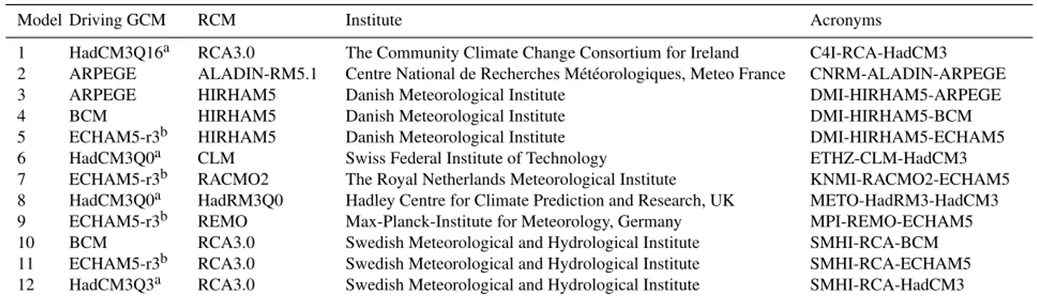
The analysis presented herein is based on a set of high-resolution climate simulations from the EU FP6 ENSEM-BLES project (van der Linden and Mitchell, 2009). In to-tal, 12 climate experiments derived from a combination of 4 GCMs and 7 RCMs, covering the period 1961–2100, were used (see Table 1). These nested GCM–RCM simulations have a horizontal resolution of ca. 25 km, a daily temporal resolution, and were forced by the IPCC SRES A1B sce-nario (Nakicenovic and Swart, 2000). We focus on the EN-SEMBLES SRES-A1B data set as to date it is the only large ensemble of high-resolution climate simulations for Europe that allows for a finer assessment of the climate model un-certainty (van der Linden and Mitchell, 2009). The A1B scenario projects a fast economic growth, global popula-tion peaking in mid-century, rapid introducpopula-tion of new and more efficient technologies, and a balance across all energy sources (Nakicenovic and Swart, 2000). The climate exper-iments were corrected for bias in the precipitation and min-imum, average, and maximum temperature fields using the quantile mapping (QM) method (Piani et al., 2010a, b; Do-sio et al., 2012). Several techniques to correct potential bias in precipitation and temperature have been recently devel-oped in literature based on different transfer functions and theoretical assumptions (Teutschbein and Seibert, 2010; The-meßl et al., 2011). We implemented the QM method be-cause it showed better performance compared to other meth-ods to correct for bias in high-resolution regional climate models (Themeßl et al., 2011). On the basis of the station-arity assumption (Christensen et al., 2008), current perfor-mance for the bias correction methods may be deemed trans-ferable to future climate. Dosio and Paruolo (2011) showed that the QM bias correction procedure drastically improved the agreement between simulated and observed climatology from the E-OBS data set (Haylock et al., 2008). Moreover, it has been shown to yield improvements in both the up-per and lower tail of the probability distribution functions (PDFs) of temperature and precipitation, with significantly positive effects on the accuracy of simulated extreme cli-matic and hydrological events (Dosio and Paruolo, 2011; Rojas et al., 2011).
Table 1.Climate simulations used to drive LISFLOOD in the period 1961–2100.
Model Driving GCM RCM Institute Acronyms
1 2 3 4 5 6 7 8 9 10 11 12 HadCM3Q16a ARPEGE ARPEGE BCM ECHAM5-r3b HadCM3Q0a ECHAM5-r3b HadCM3Q0a ECHAM5-r3b BCM ECHAM5-r3b HadCM3Q3a RCA3.0 ALADIN-RM5.1 HIRHAM5 HIRHAM5 HIRHAM5 CLM RACMO2 HadRM3Q0 REMO RCA3.0 RCA3.0 RCA3.0
The Community Climate Change Consortium for Ireland Centre National de Recherches Météorologiques, Meteo France Danish Meteorological Institute
Danish Meteorological Institute Danish Meteorological Institute Swiss Federal Institute of Technology The Royal Netherlands Meteorological Institute Hadley Centre for Climate Prediction and Research, UK Max-Planck-Institute for Meteorology, Germany Swedish Meteorological and Hydrological Institute Swedish Meteorological and Hydrological Institute Swedish Meteorological and Hydrological Institute
C4I-RCA-HadCM3 CNRM-ALADIN-ARPEGE DMI-HIRHAM5-ARPEGE DMI-HIRHAM5-BCM DMI-HIRHAM5-ECHAM5 ETHZ-CLM-HadCM3 KNMI-RACMO2-ECHAM5 METO-HadRM3-HadCM3 MPI-REMO-ECHAM5 SMHI-RCA-BCM SMHI-RCA-ECHAM5 SMHI-RCA-HadCM3
aRepresent three versions of the HadCM3 model with perturbed parameterization impacting the simulated climate response sensitivities: Q0 (reference), Q3
(low-sensitivity) and Q16 (high-sensitivity) (Collins et al., 2006).bRepresent one run of the ECHAM5 model using three different sets of initial conditions defined as “-r1”, “-r2”, and “-r3” (Kendon et al., 2010).
to determine water withdrawal and consumption in different sectors (domestic, tourism, energy, manufacturing, irrigation and livestock). The water use scenario was taken from the SCENES project (Kämäri et al., 2008, Kok et al., 2011), which aimed at developing and analyzing a set of compre-hensive water-related scenarios for Europe through a partic-ipatory process. Four comprehensive scenarios were devel-oped: Economy First (EcF), Fortress Europe (FoE), Policy Rules (PoR), and Sustainability Eventually (SuE). The sce-narios include consistent projections of the main drivers such as total population, GDP (gross domestic product), thermal electricity production, agricultural production as well as in-formation on technological changes. The EcF scenario was selected as it is the most coherent with the IPCC SRES A1B. It is characterized by a globalized and liberalized economy pushing the use of all available energy sources accompanied by a marked agricultural intensification. The adoption of new technologies and a water-saving consciousness is low result-ing in an increasresult-ing water demand of all water-related sec-tors. Only water ecosystems providing ecological goods and services for economies are preserved and improved (Kok et al., 2011).
Within SCENES, water uses for the different sectors are modeled on an annual basis, except for the irrigation water use which has a monthly temporal resolution. Note that the SCENES scenarios run until 2050. For the remaining period it was assumed that water consumption remains unchanged from 2050 onwards.
2.2 Hydrological modeling
River discharge simulations for different climate experiments (see Table 1) were obtained using the LISFLOOD model (van der Knijff et al., 2010). Being a fully distributed and physically based hydrological model developed for large-scale impact assessment studies, LISFLOOD simulates the spatial and temporal patterns of catchment responses as a
function of spatial information on meteorology, topography, soils, and land cover. It has been specifically set up for Euro-pean catchments by optimally exploiting several databases that contain pan-European information on soils (King et al., 1994; Wösten et al., 1999), land cover (European Envi-ronment Agency, 2002), topography (Hiederer and de Roo, 2003) and meteorology (Rijks et al., 1998). LISFLOOD is a GIS-based hydrological model where processes such as infil-tration, water consumption by plants, snowmelt, freezing of soils, surface runoff and groundwater storage are explicitly accounted for at the grid level. Spatial properties for soils, vegetation types, land uses, and river channels constitute the basic input information to set up a LISFLOOD run, whereas data on precipitation, air temperature, potential evapotran-spiration, and evaporation from water bodies and bare soil surfaces are the main meteorological drivers.
Potential evapotranspiration and evaporation rates are cal-culated from vapor pressure, wind speed, radiation (so-lar+thermal), albedo, and average, minimum, maximum and dew point temperature through the offline LISVAP pre-processor based on the Penman–Monteith equation (van der Knijff, 2008). We point out that variables such as dewpoint temperature, solar and thermal radiation that are employed together with the bias-corrected temperature fields to calcu-late the evapotranspiration components driving LISFLOOD are not corrected for potential bias. This could violate the en-ergy balance and potentially introduce bias in the simulated hydrological patterns (e.g., Rojas et al., 2011; Hagemann et al., 2013). However, experiments performed using the same bias correction method with a different impact model showed that the relative values of projected hydrological change are very similar if other climate variables are also bias corrected (Haddeland et al., 2012). Thus, we can reasonably presume that the impact of these inconsistencies is generally rather small.
particularly in smaller catchments. This is relevant especially in light of the increasing number of reservoirs becoming op-erational in the catchments during last decades (Svensson et al., 2005). However, such structures have not been imple-mented in our assessment due to the lack of suitable infor-mation on dams, artificial reservoirs and their current and future operation. As such, the actual magnitudes of the low-flow measures derived herein reflect more the conditions in undisturbed catchments. However, it can be argued that, un-less considerable alterations in flow regulation take place to mitigate the severity of extreme low-flow conditions, re-sults expressed in terms of relative changes in low flows are reasonably representative. LISFLOOD was calibrated using at least four years of historical river flow data in the pe-riod 1995–2002 in 258 catchments and sub-catchments dis-tributed throughout Europe. For a more detailed description of the processes and equations of LISFLOOD, as well as of its calibration, we refer the reader to van der Knijff et al. (2010) and Feyen et al. (2007, 2008).
Prior to forcing the LISFLOOD model, the climate simula-tions were re-gridded to the 5 km LISFLOOD grid employ-ing a nearest neighbor approach on the basis of the center points of the 25 km grid cells of the RCMs. The water use data were similarly re-gridded from their 5 arcmin grid to the LISFLOOD grid. The WaterGAP3 monthly (for irrigation) and annual (for the other sectors) water consumption data were equally distributed over the days in each month or year, respectively, and accounted for in LISFLOOD as a daily loss term. LISFLOOD was then run with a daily time step for a simulation period between 1961 and 2100. As such, for each experiment (climate ensemble member combined with or without water use) 140 yr of daily discharges were pro-duced at each river pixel. To analyze changes over this pe-riod, time slices of 30 yr were considered, further herein re-ferred to as control period (1961–1990), 2000s (1981–2010), 2020s (2011–2040), 2050s (2041–2070), and 2080s (2071– 2100). For each period a flow duration curve (FDC) was de-rived in each river pixel from the 30 yr simulated discharge time series. FDC represents the percentage of time that river flow is likely to exceed some specified value and has been used herein as the basis for the calculation of the low-flow indices detailed below.
2.3 Indices of streamflow drought
Various drought indices have been developed to monitor and quantify droughts. For an extensive overview on low-flow and drought indices and their derivation we refer the reader to Smakhtin (2001), Tallaksen and van Lanen (2004) and Mishra and Singh (2010). In this work we follow the ap-proach of Feyen and Dankers (2009) and focus on two impor-tant aspects of a drought, namely magnitude and persistence through time.
Firstly, we analyze low flows through the magnitude of the river discharge, expressed here by the 7 day minimum
flow (qmin) at several recurrence intervals. We apply a 7 day averaging to focus on the general behavior of streamflow dynamics and to cancel the day-to-day fluctuations in river flow, which are often arbitrary or artificial in low-flow pe-riods (Tallaksen and van Lanen, 2004; Lehner et al., 2006). From the smoothed discharge series the annual minima are selected, through which a generalized extreme value (GEV) distribution is fitted using the maximum likelihood (ML) method (Gilleland and Katz, 2005). From the fitted GEV distribution qmin values for different return periods ranging between 2 and 100 yr are derived in each river pixel.
Secondly, we consider the development in time of drought events by evaluating deficit characteristics of periods in which discharge stays below a threshold flow. Deficits can be evaluated in terms of their run duration (length of event) and severity (cumulative deficit or negative run sum) (Smakhtin, 2001). However, given the often strong correlation between drought durations and deficit volumes (Woo and Tarhule, 1994) and considering that the latter are a more effective measure of the magnitude of water shortage relevant for oper-ational water management (Tallaksen and van Lanen, 2004), we focus only on deficit volumes (def). The threshold for evaluating deficits can be defined as a percentage of the mean flow or as an exceedance frequency of the FDC. We opt for the latter, such that everywhere in Europe discharge time se-ries fall below the threshold an equal number of days, but al-lowing deficit volumes to vary according to location-specific conditions. As a balance between representing low-flow con-ditions and assuring sufficient events for extreme value fit-ting (Tallaksen et al., 1997; England et al., 2004; Fleig et al., 2006) we apply the 80 % exceedance frequency of the FDC (further referred to asQ80), as constant threshold. We note that for the future time slices, deficits are evaluated against the threshold from the control period (1961–1990). Using the ML method, in each river cell a generalized Pareto (GP) dis-tribution was then fitted through the partial duration series of deficit volumes representing the shortfalls below the thresh-old. From the fitted distribution, deficit volumes for recur-rence intervals ranging between 2 and 100 yr were derived.
dependent droughts. As not all minor events were excluded after the 7 day MA procedure, in each river cell we addition-ally removed all events with a deficit smaller than 0.5 % of the maximum deficit in that cell, following Zelenhasic and Salvai (1987).
2.4 Streamflow regimes in Europe
Streamflow regimes across Europe vary strongly due to the large variability in climatologic conditions and local factors that influence the hydrological response, such as the pres-ence of aquifers, variations in soil properties and land cover. In regions with a cold climate, typically winter and summer droughts can be differentiated (e.g., Fleig et al., 2006; IPCC, 2012). In winter, most water is trapped as snow and ice, of-ten resulting in the lowest flows seen throughout the year. Hence, by applying an annual analysis there is the risk that low flows in the frost-free season, originating from negative imbalances in precipitation, are not accounted for, or that the sample of events used for extreme value fitting find their ori-gin in different physical processes. The latter also violates the underlying theory of frequency analysis, namely that the events are considered to be drawn from an independent and identically distributed (iid) random variable.
Following Hisdal et al. (2001) and Feyen and Dankers (2009) we distinguish between a nonfrost and frost season, where the latter is defined for each river pixel as the period of the year in which the monthly average temperature in the upstream area drops below zero in at least 23 out of 30 yr (reference length of time slices). By averaging over the upstream area we avoid labeling river pixels as nonfrost when in large parts of the upstream catchment water is still stored as ice or snow. This is especially the case for downstream river reaches in areas with pronounced topography, such as for the major streams that drain from the Alps (e.g., Rhine, Rhone, or Po rivers). Thus, time series of daily discharges are split up in nonfrost and frost seasons according to the afore-mentioned criterion. Streamflow drought indices are estimated separately for each season. Note that for deficit volumes we use differentQ80 threshold values calculated from the FDCs corresponding to the respective season.
For intermittent and ephemeral streams the data series of annual minima may contain several zero values, hence dis-continuous probability distribution functions need to be ap-plied for inferring low-flow probabilities. Analysis of the LISFLOOD simulations showed, however, that for catch-ments with an upstream area larger than 1000 km2 the time series of annual minima did not contain any zero flow val-ues, and thus can be considered to be perennial under current and future climatic conditions. We therefore limit the analy-sis to river basins with an upstream area exceeding 1000 km2, hereby excluding ephemeral rivers. Even if the latter (head-water and lower order streams) are particularly sensitive to climate change, as analyzed in a comprehensive review by
Brooks (2009), to be properly quantified they would require a finer hydro-geomorphological characterization than the one provided in the large-scale approach presented herein. Fur-thermore, we argue that river basins with an upstream area exceeding 1000 km2are representative enough to explore the impact of climate changes on future hydrological droughts at continental scale.
2.5 Uncertainty in low-flow projections
2.5.1 Climate uncertainty
Climate models are the most robust tools available to gener-ate consistent climgener-ate change projections. However, they are still a source of considerable uncertainties due to the incom-plete, missing or incorrect representation of some physical processes and approximated parameterizations (e.g., Katz, 2002; Murphy et al., 2004; Déqué et al., 2012). One of the crucial issues emerging from recent studies (see, e.g., Chris-tensen and ChrisChris-tensen, 2007; van der Linden and Mitchell, 2009) is that different climate experiments may still show large variations in the simulated variables, especially for pre-cipitation. This may be translated to the impact models, of-ten resulting in considerable climate-induced variability in impact estimates.
Model uncertainties can be partly resolved using an ensemble-based framework where simulations from differ-ent climate models are used to drive the impact assessmdiffer-ent model. Projections based on a multi-model ensemble can be considered more indicative than projections produced by single models alone, as the multi-model average or median can be expected to outperform individual ensemble mem-bers, thus providing an improved “best estimate” projection (IPCC, 2007, Stahl et al., 2011; Gudmundsson et al., 2012). On the other hand, it should be noted that a multi-model ensemble, especially when the sample is relatively small, may still be affected by extreme or outlier ensemble mem-bers. Also, over the ensemble, errors in one process or pa-rameterization may be compensated by errors in other pro-cesses or parameterizations (e.g., Murphy et al., 2007). The weighting of climate simulations as an approach to com-bining climate information is subject to considerable debate (e.g., Christensen et al., 2010; Coppola et al., 2010; Déqué and Somot, 2010). Any weighting method depends on sub-jective choices about the metrics and combining procedure into an overall weight for the individual models. Such fac-tors will determine the spread in the climate and impact es-timates and add an additional layer of uncertainty. There-fore, climate simulations of the different ensemble mem-bers have been equally weighted when summarizing the low-flow projections.
members in terms of showing a decrease or increase in low-flow measure of at least 5 % with respect to the control period.
The statistical significance of the changes for the projec-tions of streamflow drought indices is evaluated by the use of Welch’st test, assuming that the variances of the control pe-riod and the different time slices are not necessarily the same (Welch, 1947; see also Von Storch and Zwiers, 1999, p. 113). Here, the test statistic can be approximated with a normalt distribution, where the appropriate degrees of freedom are estimated from the data. If the resultingp value is smaller than a predefined significance level, e.g., 5 % (α=0.05), the ensemble mean in the future time slice is said to be signif-icantly different from that in the control period given the climate uncertainty.
2.5.2 Extreme value fitting uncertainty
The aim of extreme value (EV) analysis is to find a paramet-ric model for the tail of the data generating process, then to fit this model to the extreme observations and use it for extrap-olation beyond the observed data. Extreme value modeling typically faces the problem of data scarcity, or that the fitting is based on a relatively small number of observations. This introduces uncertainty in the estimation of the return levels that depends on the quantity of data in relation to the degree of extrapolation. Here this uncertainty has been appraised by applying the profile-likelihood method (Coles, 2001) on the return levels of the GEV and GP distributions and estimat-ing the correspondestimat-ing 95 % confidence intervals. The profile-likelihood has proven to be more robust and able to better capture the usual asymmetric nature of the confidence in-tervals than other conventional methods (e.g., delta method) (Coles, 2001; Beirlant et al., 2004).
We note that recent studies have shown that hydrological uncertainty may further increase the variability of projections in water resources (Gudmundsson et al., 2012; Hagemann et al., 2013), in particular in the low-flow spectrum as sug-gested by the considerable discrepancy between large-scale hydrological models in the evaluation of drought propaga-tion (Van Loon et al., 2012). Hydrological components may, however, be differently affected by modeling uncertainties. For instance, Hagemann et al. (2013), using multiple global climate and hydrology models, suggests that uncertainty in the projected changes in evapotranspiration is largely dom-inated by the spread due to the choice of the hydrological models, whereas uncertainty in runoff changes mainly origi-nates from the choice of the climate model. In contrast, other studies have shown the limited relevance of hydrological un-certainty compared to unun-certainty arising from climate mod-els (e.g., Wilby, 2005; Najafi et al., 2011). Even if hydrolog-ical modeling could potentially introduce additional sources of uncertainty in the projections of streamflow droughts, an attempt to account for the hydrological uncertainty is beyond the scope of our analysis. Moreover, the quantification and
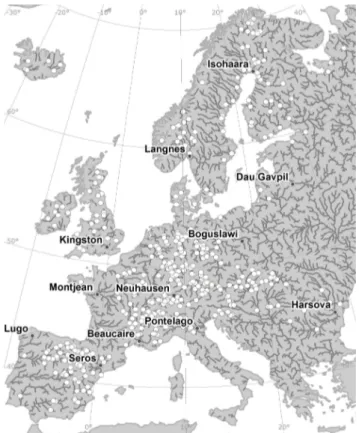
Fig. 1.Location of the 446 gauging stations used to evaluate simu-lated streamflow drought indices. Filled black circles show valida-tion stavalida-tions used in Figs. 5, 6 and 12.
modeling of environmental, social, and policy drivers of wa-ter use – such as population dynamics, land use changes, and agricultural, industrial, energy and environmental policies – as well as economic and technological developments, are in-herently uncertain (Kok et al., 2011). Therefore actual wa-ter consumption could deviate from the SCENES projections used herein.
3 Results and discussion
3.1 Validation of low-flow simulations
As shown in Fig. 1, the validation stations are not evenly distributed across Europe, with a high density of stations lo-cated in western and central parts of Europe and hardly any in Italy and southeastern Europe. At 338 stations the number of years with a frost season in the control climate was at least 23 out of 30; hence they were used for validation in both the nonfrost and frost season analysis.
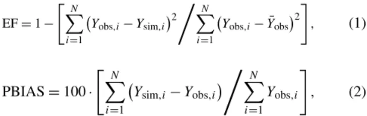
Control climate simulations do not reproduce the histor-ical weather of the 1961–1990 period, but only the aver-age climate conditions. This does not allow a day-to-day or event-to-event comparison. Instead, we evaluate the accuracy of the LISFLOOD simulations by comparing observed and simulated low-flow indices over 1961–1990 through statisti-cal measures. More specifistatisti-cally, we employ model efficiency (EF), and percent bias (PBIAS), defined as
EF=1−
"N X
i=1
Yobs,i−Ysim,i 2
,N X
i=1
Yobs,i− ¯Yobs 2
#
, (1)
PBIAS=100·
" N X
i=1
Ysim,i−Yobs,i
, N X
i=1
Yobs,i
#
, (2)
whereYobs,i andYsim,i are the observed and simulated
low-flow index at stationi=1,. . . ,N=446, respectively, and the horizontal bar denotes averaging over all stations. EF de-termines the relative magnitude of the simulated error vari-ance compared to the observed data varivari-ance. It ranges be-tween minus infinity and 1.0, with higher values for increased model performance. PBIAS measures the average tendency of the simulations to be larger or smaller than observations. It ranges from−100 to+100 with low-magnitude values (close to 0) indicating accurate model prediction, whereas positive (negative) values indicate overestimation (underestimation). Note that theQ80 threshold for the analysis of deficit vol-umes is separately calculated for the observed and simulated time series, which implies that the validation is based on relative differences in deficit volumes.
Figure 2 presents the performance of the 12 ensemble members to reproduce average annual 7 day minimum flows in the control period. Results show a good performance across the climate simulations with EF values ranging be-tween 0.81 and 0.95. Two common features can be ob-served for all members of the ensemble. Firstly, at some sta-tions the simulated minimum flows deviate strongly from those derived from observations, a behavior that is more pronounced with decreasing catchment size (note that lower (bigger) discharges generally correspond to smaller (larger) catchments). This relates to multiple sources of uncertainty that are more dominant in small basins. These include, among others: intrinsic limitations of RCMs to reproduce small-scale processes; conceptual approximations in the LIS-FLOOD model, its input data and parameterization; not fully accounting for reservoirs/lakes and flow regulation in the modeling setup; and measurement errors at river gauging
stations. The lower model performance for smaller catch-ments implies that future projections of changes in low-flow conditions presented herein should be interpreted more cau-tiously compared to those obtained for larger catchments. We also note that by coupling offline RCM simulations with the hydrological model, as well as by correcting the bias only in temperature and precipitation, the energy and water bal-ance are not necessarily preserved. Notwithstanding the lat-ter, Rojas et al. (2011) showed the strong improvement in LISFLOOD performance after bias correcting temperature and precipitation.
Secondly, there is a general tendency to underestimate ob-served minimum flows, as expressed by the negative val-ues of PBIAS (ranging between −13 and −40.5 %). This is most likely related to the underestimation of the low-end percentiles of the bias corrected precipitation, and a poten-tial overestimation of the number of dry days obtained from the fitting of the transfer functions (Dosio and Paruolo, 2011; Rojas et al., 2011). The omission of reservoirs in the hydro-logical simulations may additionally contribute to the under-estimation of the modeled streamflow drought conditions.
Figure 2 also shows that models with a large bias do not necessarily show a low performance based on model effi-ciency. This suggests that different ensemble members may provide higher accuracy with respect to simulating differ-ent aspects of the low-flow spectrum, which reinforces the idea of a multi-model framework as the basis for streamflow drought impact assessment due to climate change. This also supports the findings of Lenderink (2010), who explored dif-ferent metrics of extreme daily precipitation to conclude that there is no metric that guarantees an objective and precise ranking or weighting of climate models.
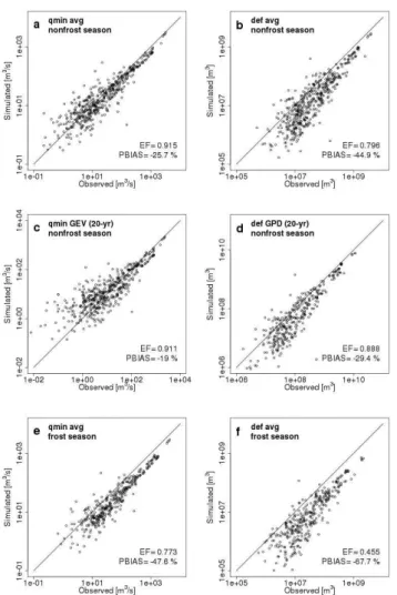
Fig. 2.Observed versus simulated average annual 7 day minimum flows for the control period (1961–1990) at each of the 446 stations depicted in Fig. 1 based on the hydrological simulations driven by the 12 climate experiments listed in Table 1.
A comparison between the statistics of the fitted extreme value distribution (here exemplified by minimum flows and deficits with a 20 yr recurrence interval) shows nearly equally good performance for the minima and deficits (Fig. 3c, d). The decreases in PBIAS observed for fitted extreme values with respect to the averages may be explained by the fact that the former includes an optimization process that mini-mizes discrepancies between observed and simulated values, thus reducing the bias. High values of EF confirm that LIS-FLOOD simulations are fairly robust in capturing the statis-tics of extreme streamflow droughts occurring in the nonfrost season.
In Fig. 3 (panels 3e and 3f) it can also be seen that LIS-FLOOD driven by control climate simulations has problems in reproducing runoff and base flow in the frost season, re-sulting in a larger tendency to underestimate the low-flow indices in comparison to the nonfrost season. This is due to a combination of several factors, including (1) concep-tual and parameter errors in the snow and frost modules of LISFLOOD that affect drainage in the cold season; (2) un-certainties in the observed winter precipitation (Goodison et al., 1998; Yang et al., 2001) used in the calibration of the
hy-drological model that may have resulted in an incorrect pa-rameterization of the groundwater reservoir; (3) too low tem-peratures during intermittent melt events, resulting in more water that remains stored as snow and less base-flow gen-eration; and (4) not properly accounting in the LISFLOOD setup for storage release from reservoirs to guarantee min-imum flow requirements, for example, for hydropower pro-duction. This may also induce artificially higher thresholds (Q80)than those derived from the simulated flow duration curve, yielding at many stations larger observed deficit vol-umes compared to those simulated, especially under severe drought conditions.
Fig. 3.Observed versus ensemble-averaged simulated streamflow drought indices for the control period (1961–1990) at each of the 446 stations depicted in Fig. 1.
LISFLOOD capabilities in simulating low flows, we derive streamflow drought indices of the future time slices (2000s, 2020s, 2050s, 2080s) for both nonfrost and frost seasons.
3.2 Changes in meteorological forcing and water
consumptions
To better understand the processes affecting future low-flow characteristics across Europe we first summarize the pro-jected changes in the main driving climatic variables. Fig-ure 4 shows for Europe the ensemble-average changes by the 2080s compared to the control climate (1961–1990) in tem-perature and precipitation for the nonfrost and frost seasons. Because streamflow at a given location depends on the hy-droclimatological conditions over the upstream river basin, these maps show average changes over the upstream area that contribute flow to that location rather than the change at the grid cell itself. Figures 5 and 6 (top 2 rows) present ensemble-average alterations in these variables throughout
Fig. 4. Ensemble-averaged changes in average temperature (top row) and precipitation (bottom row) between 2080s and control pe-riod for nonfrost (left column) and frost (right column) seasons. The change at each location reflects the average change over the upstream area contributing flow to that location. In the frost sea-son panels, areas shaded in light gray represent regions with a frost season in the control climate and without a frost season in the ensemble-average scenario climate, while dark gray areas indicate regions with no frost season both in the control and scenario peri-ods.
the year at a selection of stations that span the range of cli-matic and hydrological conditions in Europe (see Fig. 1).
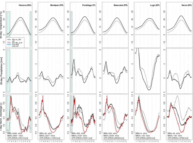
Fig. 5.Inter-annual dynamics in temperature (top row), precipitation (middle row) and 7 day average streamflow (bottom row) at a selection of stations (see Fig. 1) in the control period (light gray lines) and 2080s (black line). Temperature and precipitation reflect 30 day upstream averages. The red line for streamflows (bottom row) reflects the scenario accounting for water use. Blue shaded areas indicate the frost season in both periods (control as light blue, 2080s as dark blue).
and altitudes) considerably in the course of the 21st century. The absence of a permanent frost period due to global warm-ing will strongly affect the hydrological cycle and ecosystem functioning in these regions.
Average precipitation in the nonfrost season is projected to decline in southern Europe, with decreases as high as 30 % in the most southern regions, to a rise of 10–20 % in northern Europe, and to remain relatively stable in a transition zone in between. Comparison of the stations plots in Fig. 6 shows that in the most southern parts of Europe (see stations Lugo and Seros) drying is much stronger in spring compared to summer, whereas further north (see stations Montjean and Beaucaire, Ponte Lago) equally strong reductions are ob-served in summer precipitation. Note that the average maps over the nonfrost season may mask some of the inter-annual changes. At Kingston station (Fig. 5), for example, average precipitation is projected to slightly increase, but summer precipitation will decrease. In the frost season average pre-cipitation is projected to strongly increase over most parts of northern Europe (e.g., stations Langnes, Isohaara and Dau
Gavpil, Neuhausen in Fig. 5), which is in line with other studies using different climate models and emission scenar-ios (see e.g., Christensen and Christensen, 2007; Räisänen and Eklund, 2012).
Fig. 6.As Fig. 5, for different stations.
and to increasing manufacturing (Flörke et al., 2011). At the same time, irrigation water requirements will play a ma-jor role in the northern Iberian Peninsula and northern Italy due to an intensification of crop production in combination with increasing temperatures induced by climate changes, and will lead to an increase of ca. 25 % in total water ab-stractions. Slight decreases in future total annual water with-drawals can be observed in some river basins in Denmark, southern Iberian Peninsula, southern Italy and Greece. In southern Iberia this is likely a result of the expected reduction in annual irrigation water consumption. Additional details on changes in water consumptions for the different sectors can be found in Flörke et al. (2011).
3.3 Projections of future streamflow droughts
3.3.1 Frost season
The bottom rows in Figs. 5 and 6 show how the changes in meteorological forcing affect the streamflow dynamics across Europe. In stations with a frost season (e.g., stations Langnes, Isohaara, Dau Gavpil, and Neuhausen in Fig. 5), low flows in this period are projected to augment consider-ably, and hence winter droughts to become less severe. In
warmer and wetter winters, a smaller portion of precipita-tion will be temporarily stored as snow or ice, resulting in increased flows in the cold season. This is in line with the findings by Räisänen and Eklund (2012) of a decrease in long-term mean snow water equivalent throughout the 21st century in northern Europe.
Fig. 7.Total annual water withdrawals aggregated to river basin scale for the control period (a) and the corresponding expected changes in the 2050s according to the EcF scenario from the SCENES project(b).
3.3.2 Future streamflow minima in the nonfrost season
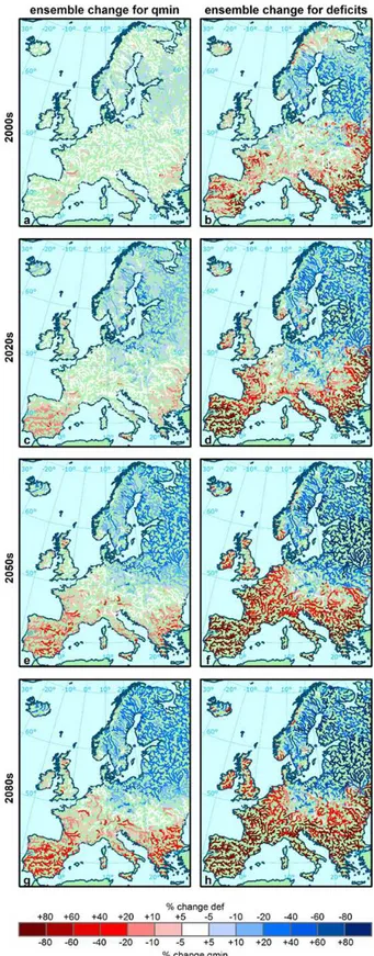
For the nonfrost season, changes in 7 day minimum flows with recurrence intervals ranging from 2 up to 100 yr were derived from the GEV distributions fitted through the annual minima series for the control and future time slices. Figure 8 (left column) shows for river pixels with an upstream area larger than 1000 km2the changes in 7 day minimum flows (qmin) with 20 yr recurrence intervals between the control and the four scenario periods. A reduction (augmentation) in minimum flows indicates increasing (decreasing) drought hazard and is displayed in red (blue) color in Fig. 8.
Hardly any changes in minimum flows can be detected be-tween the control period and 2000s in part due to the 10 yr overlap between the two time slices. By the 2020s, the most southern areas of Europe (Iberian Peninsula and southeast-ern Balkans) first start to see a reduction (10–20 %) in mini-mum flows. Progressing further in time, streamflow droughts in the south will gradually intensify and the areas negatively affected will expand further north, covering most of south-ern and westsouth-ern parts of Europe by the end of this century. The Iberian Peninsula, Italy, and the Balkan region will be most affected, with reductions in minimum flows of up to 40 % by the 2080s, but also France and to a lesser extent the United Kingdom, Ireland and Belgium will experience lower minimum flows.
Lower minimum flows in future time slices result from the combined effects of reduced precipitation and increased evaporative demands with higher temperatures (e.g., Fig. 6, stations Lugo, Seros and Beaucaire). Actual evapotranspi-ration rates, however, are not necessarily higher, as they may be limited by lower soil and subsurface storage. Sim-ilar changes in streamflow droughts have been detected in southern parts of Europe by Lehner et al. (2006) and Feyen and Dankers (2009), even if they utilized different emission scenarios and climate simulations.
Although not shown here, the large spatial pattern of changes in Fig. 8 is similar for minimum flows at other re-turn periods. However, in some regions (United Kingdom,
Germany, Benelux, France, northern Italy and eastern parts of Europe) the reductions in minimum flows are relatively more severe for smaller return periods. This relates to the projected changes in the seasonality of precipitation. These regions will experience strong reductions in precipitation in summer and a less important decline in autumn, whereas precipitation will increase strongly in winter and mildly in spring (see e.g., stations Kingston, Beaucaire, Montjean and Pontelago in Figs. 5 and 6). Droughts in these regions are typically a summer or autumn phenomenon. Minimum flows with relatively short recurrence intervals, which reflect the water balance in the preceding months, are strongly impacted by the pronounced decrease in summer and autumn precipi-tation. The rarer events, on the other hand, reflect imbalances in precipitation over longer time spans, in which the reduced precipitation input over summer and autumn is counterbal-anced by increased subsurface storage at the start of the sum-mer season due to elevated precipitation amounts in winter and spring.
In northern parts of Europe an opposite signal is observed in the non-frost season and minimum flows prevalently in-crease (or become less severe) in time. Scandinavia and the Baltic countries will experience a general increase in 20 yr minimum flows of up to 20 % – in some inland tributaries up to 40 % – by the end of the 21st century. This is a re-sult of the increase in precipitation that outweighs the effects of increased evapotranspiration demands with higher tem-peratures. Here the change to less severe droughts is more pronounced for rarer events due to the considerable increase in precipitation during the frost season, which after melting of snow in spring yields larger volumes of water stored in the subsurface at the start of the summer season. In some high-latitude areas, however, the projected rise in winter pre-cipitation may not necessarily result in thicker snowpacks, which in combination with earlier snowmelt may result in relatively stable minimum flows in the frost-free season (e.g., some southern parts of Sweden and along the west coast of Norway).
3.3.3 Future streamflow deficits in the nonfrost season
Changes in 7 day streamflow deficits with return periods ranging between 2 and 100 yr were obtained from the fit-ted GP distributions for deficit volumes in both the control and scenario time slices. We present changes in 20 yr deficits (def) (Fig. 8, right column) for river pixels with upstream catchment size exceeding 1000 km2. Note that in this case red colors indicate an increase in flow deficits, which implies more severe shortfalls below the threshold (Q80 of control period) or more severe droughts.
In the nonfrost season flow deficits are projected to be-come more severe in most of Europe, except in northern and northeastern regions. In many regions of the Mediterranean – including the Iberian Peninsula, Italy and the Balkans – as well as parts of eastern Europe – including Bulgaria and
Ro-mania – 20 yr deficit volumes are expected to increase by 50 % by the 2020s. These regions will experience contin-ued drought intensification up to the end of the century, with deficit volumes (belowQ80of the control period) increasing by up to 80 % by the 2080s. From the 2050s onwards most of France, the Netherlands, Belgium, United Kingdom and the Alpine regions will also be prone to more severe stream-flow deficits (increases between 20 and 50 %). Although not shown here and in agreement to what was observed for the minimum flows, events with shorter recurrence intervals show stronger increases in deficit volumes (mainly in south-western parts of Europe). It should be noted, however, that the extrapolation error when fitting the extreme value distri-bution beyond the length of the time series increases with recurrence interval. Hence, projections for higher return pe-riods are more prone to uncertainty, which also explains the somewhat more scattered pattern in the changes of deficit volumes for higher return periods in some regions.
In northeastern Europe, including the Baltic countries, flow deficits in the nonfrost season show a declining trend, with reductions in deficit volumes of up to 60 % and more by the end of this century. Northwestern parts of Europe display a decreasing trend in deficit volumes, but locally (e.g., along the Norwegian west coast, areas in southern Sweden) the changes show higher spatiotemporal variability with sparse rivers showing an opposite tendency in the signal of change. This mixed pattern is due to the combined effects of a general increase in precipitation and reduced snowmelt contribution caused by less accumulation of snow in winter. Depending on the relative magnitude of these processes in future time slices, streamflow deficits in this region may either become more or less severe.
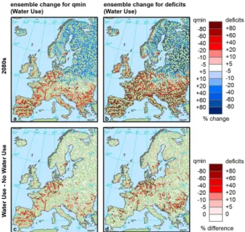
Fig. 9.Ensemble-average change in 20 yr return level minimum flow and deficit volumes due to climate change and water consump-tion between the 2080s and the control period (top row) and cor-responding differences with ensemble-average changes driven only by climatic drivers (bottom row).
Similarly, rarer deficit volumes (i.e., with higher recurrence intervals) are therefore less affected at midlatitudes.
3.3.4 Impact of water consumption on streamflow
droughts in the nonfrost season
The results described above only show the effect of climate change on low-flow characteristics. The impact of increased water consumption on low-flow characteristics is presented in Fig. 9, which shows the ensemble-average change be-tween the 2080s and the control period in 20 yr minimum flows and deficit volumes when accounting for both climate change and water consumption (Fig. 9a, b). It is worth not-ing that the 7 day-average streamflow accountnot-ing for both climate change and water use is also included in Figs. 5 and 6 as a red line in the bottom row panels. Note that to account for water consumption, LISFLOOD was coupled on a daily time step with WaterGAP3 for the whole simulation period 1961–2100, hence the changes in low flows with respect to the control period reflect the combined effects of alterations in climate and consumptive water use. The bottom panels in Fig. 9 show for each drought index the difference between the ensemble-average changes driven by changes in climate and water use and those accounting only for the climatic ones for the 2080s.
Intensive water consumption as projected by the EcF sce-nario will further aggravate streamflow droughts in many re-gions of Europe. It will negatively affect both minimum flows and deficit volumes in central, western and eastern Europe
due to the projected increases in water abstractions (com-pare with Fig. 7). In some regions where no or slightly pos-itive changes in low-flow conditions are induced by climate change, increasing water consumption will reverse this trend and lead to more severe streamflow droughts. This behavior is most notable in the Benelux countries, western Germany, northwestern France (see station Montjean in Fig. 6), and lo-calized parts in the United Kingdom (see station Kingston in Fig. 5), and in central and eastern European countries (Slovakia, Czech Republic, Hungary and Romania). Water use abstraction will exacerbate minimum low-flow condi-tions by ca. 10–30 % over the Mediterranean regions, espe-cially where maximum rates of seasonal water demand of irrigated crops overlaps with drier periods (see e.g., stations Seros, Lugo, Ponte Lago and Beaucaire in Fig. 6). This sug-gests that even in front of a relative reduction in total annual water abstractions (compare with Fig. 7), the combined ef-fects of alterations in climate and human water consumption will strongly aggravate streamflow drought conditions. In re-gions with a positive effect of warming on low-flow condi-tions, such as the Scandinavian Peninsula and Baltic coun-tries, intensive water use may reduce future low flows, but not sufficiently to offset the positive effect.
3.4 Uncertainty in projections of streamflow droughts
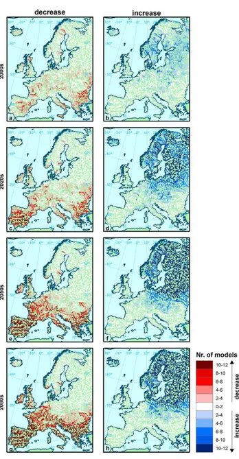
Figure 10 presents the consistency amongst the 12 ensemble members in projecting a decrease (left panels) or increase (right panels) in minimum flows in future time slices with respect to the control period. Similar patterns are found for deficits and are not shown here for brevity. For the 21st cen-tury, the majority of hydrological simulations depict con-sistently increasing streamflow drought conditions over the Iberian Peninsula, France, Italy, the United Kingdom and southern Balkan region. On the other hand, models also agree well about the decrease in streamflow droughts in northeast-ern Europe, Scandinavia, the Baltic countries, and northnortheast-ern parts of Poland. A more mixed pattern with higher variabil-ity in low-flow regimes across streamflow drought simula-tions is evident mainly over the transition zone across central Europe and the Carpathians. A common feature for the min-imum flow and deficit indicators is the improved agreement in time between projections of the ensemble members in the aforementioned areas, thus, suggesting a stronger signal-to-noise ratio as time proceeds.
Fig. 10.Consistency of the streamflow drought simulations for dif-ferent time slices indicated by the number of simulations (out of 12) agreeing in a decrease (left) or increase (right) of more than 5 % in minimum flows.
statistically significant at the 5 % level (α=0.05). In those areas where the ensemble-average changes in low-flow mea-sures are small, higherp values are found, thus suggesting a weaker signal-to-noise ratio. This indicates that the mod-els tend to show less agreement (see also Fig. 10) about the direction (and magnitude) of change in the transition zone between clearly defined regions with increasing (south) and decreasing drought hazard (north). Although not shown here, the same behavior was observed when water consumption is accounted for.
The high consistency amongst the different climate mem-bers in projecting streamflow drought changes – already
Fig. 11.pvalue to test significance of the average change in min-imum flows (left) and deficit volumes (right) between the corre-sponding time slices and the control period (1961–1990).pvalues are obtained on the basis of Welch’sttest.
evident in the near-future (Fig. 10c, d) – suggests that the decadal-scale internal climate model variability, which may partially or completely obscure the climate signal in extreme events, is of secondary importance and progres-sively decreases as time proceeds. Low flows largely de-pend on imbalances in precipitation over monthly to seasonal timescales, rather than on single events as is the case for example for floods (Rojas et al., 2012). At these scales the changes in rainfall that determine the drought hazard are well established and more consistent between climate models.
Fig. 12.Inter-annual dynamics in simulated 7 day streamflow for the control period and the 2080s for selected stations (see Fig. 1). The thin blue and red lines represent the ensemble averages for the control and 2080s, respectively. The corresponding shaded areas show the spread amongst ensemble members within the respective period.
daily minimum, maximum and average discharges are calcu-lated. The area shaded in light purple and the blue line show the spread (range between maximum and minimum simu-lated value) and average for the control period, respectively. The area shaded in orange in combination with the red line represents this information for the 2080s. In general the vari-ability amongst the ensemble members is most pronounced in the high ranges of the flow spectrum, which relates to the inconsistency amongst the models in the representation of extreme precipitation events (Rojas et al., 2012). At all sta-tions, except for Seros, the ensemble spread increases with time compared to the control period, indicating some diver-gence in the magnitude of the signals projected by the differ-ent ensemble members. We also observe a large variability in spread across the stations, with the highest uncertainty both in the control period and the 2080s at stations Dau Gavpil and Boguslawi. This suggests a higher variability in simulated climate in this region, or a higher sensitivity of the hydro-logical model to climate variability. The latter may be linked to the limited number of stations in this part of Europe used for the calibration of LISFLOOD. Notwithstanding the large uncertainty in the ensemble and the overlap (area shaded in dark purple) in spread for the two periods, the
ensem-ble averages still show a clear trend towards increasing low flows (in both seasons) at these stations. At the Harsova and Neuhausen stations, in the nonfrost season the control period spread falls nearly fully within the spread of the 2080s, sug-gesting that individual members of the ensemble may show opposite signals of change. This is also expressed by the high pvalue (hence low significance of change, see Fig. 11) and lower consistency between ensemble members (see Fig. 10) at these locations. The same behavior is observed at Kingston station, although the absolute spread in both periods is much smaller. At stations in southern Europe (see e.g., Montjean, Beaucaire and Lugo and Seros), (nearly) all ensemble mem-ber low-flow simulations for the 2080s fall below those of the control period, hence showing a clear increase in severity of low flows in the nonfrost season. At the most northern sta-tions (Langens and Isohaara), the opposite can be observed in the frost season, where all ensemble member low-flow sim-ulations clearly show less severe streamflow drought condi-tions in the future. In the nonfrost season, more overlap of the spread can be observed, but a clear increase in ensemble-average low flows is still observed at these stations.
Fig. 13.Relationship between the magnitude of climate change (CC) and EV fitting (Fit) uncertainties over the 446 gauging stations (see Fig. 1) for the control and 2080s periods and for the 2 and 100 yr return periods. Colors of points refer to the magnitude of return levels (rl). GEV results for minimum flows shown in panels(a)through(e), while GP results shown in panels(f)through(j).
panels visually exemplify the uncertainty sources in the EV analysis of annual minimum flows and deficits derived from the hydrological simulations obtained from the differ-ent members of the climate ensemble (Fig. 13a and f, re-spectively). The dark gray area reflects the uncertainty aris-ing from employaris-ing alternative climate simulations to force LISFLOOD (CC uncertainty), where the thick black line rep-resents the ensemble average of the fitting distribution (rl). The light gray area, on the other hand, reflects the additional uncertainty arising from the extreme value fitting (Fit uncer-tainty) and is expressed by the 95 % confidence intervals on the return levels averaged on the twelve hydrological simu-lations. Marginal uncertainty of fitting (MUF) is calculated as the ratio of uncertainty fitting over the total uncertainty – including climatic and fitting sources – for a given
re-turn period. Right panels in Fig. 13 show the relationship between the magnitude of CC and Fit uncertainty (on the x andy axes, respectively) for all stations (minimum flows and deficit are shown in Fig. 13b–e and Fig. 13g–j, respec-tively). Point colors refer to the magnitude of return levels (rl), whereas avg(MUF) represents the marginal uncertainty of fitting averaged over all stations.
uncertainty along an increasing return period, especially for stations with lower return levels, as exemplified by the cor-responding reduction in average MUF. This suggests that the variability of projections of most extreme low-flow events is more influenced by the climate model variability than the fit-ting confidence. Projections of minimum flows indicate an overall increase in magnitude of uncertainties for both cli-mate and fitting. However, fitting uncertainty is expected to play a secondary role with respect to the climate uncertainty as shown by the reduction in average MUF in the 2080s compared to the control period.
Uncertainty in the GP fitting plays a more important role for the deficit volumes than for the minimum flows, as quan-tified by higher average MUF ranging from 38 to 60 % (Fig. 13g–j). The GP fitting to the deficit volumes is sus-ceptible to errors as partial duration series of deficits be-low a threshold often contain, even after smoothing the dis-charge series as applied here (see Sect. 2.4.), a large num-ber of minor droughts that distort the inference of the scale and especially the shape parameter of the GP distribution. This may result in fitted GP distributions that rapidly over-shoot the underlying data used for fitting. Even if the mag-nitude of both climate and fitting uncertainties increase in future time slices, the average MUF tends to decrease in fu-ture projections of deficits, consistently to what is observed for the minimum flows. This confirms that extreme value fit-ting of annual minima and deficit volumes may introduce ad-ditional sources of uncertainty in projections of streamflow droughts playing, however, a secondary role with respect to the climate uncertainty.
4 Conclusions
Here we have assessed the implications of global warming and water consumption on low-flow conditions in Europe. We first generated an ensemble of streamflow scenarios from 1961 to 2100 that account for future climate developments – and the climate model uncertainty therein – under the IPCC SRES A1B scenario, as well as for changes in consumptive water use under a coherent scenario (Economy First, FP6 SCENES project). In a second step, streamflow drought in-dices were derived using extreme value analysis and changes between different 30 yr windows were analyzed.
Our analysis has led to the following three main conclu-sions.
The first conclusion is that due to global warming many river basins in Europe are likely to be more prone to severe water stress. Mostly affected will be southern parts of Eu-rope, where droughts are projected to become considerably more severe over the 21st century. Minimum flows may be lowered by up to 40 % only due to climate change in the Iberian Peninsula, southernmost regions in France, Italy and the Balkan region. Streamflow deficits, reflecting shortfalls below a threshold flow, show even larger changes in these
re-gions, with increases in severity of the events by up to 80 %. Also western and central parts of Europe will become more negatively affected and see more severe low-flow conditions. In northern parts of Europe, droughts originating from pre-cipitation anomalies are projected to become considerably less severe.
A second conclusion is that intensive water consumption will aggravate streamflow drought conditions by 10–30 % in southern, western and central Europe, and to a lesser extent also in the United Kingdom. Some regions subject to little or small positive impacts of climate change, may actually see this trend reversed by intensive water use, leading to more severe drought situations. This is the case for large parts of the Benelux, northwestern Germany, northwestern France, and localized parts of the United Kingdom and central and eastern European countries (Slovakia, Czech Republic, Hun-gary and Romania). We note that in this study only changes in climatology and water consumption are considered. Land use dynamics and consequent changes in vegetation char-acteristics (e.g., leaf area index) may affect evapotranspira-tion as well as soil moisture redistribuevapotranspira-tion and groundwater recharge, and consequently the development of droughts.
A third conclusion is that the model projections are fairly consistent amongst the different climate ensemble members. This results in projected strong signals for southern (nega-tive signal, or more severe droughts) and northern (posi(nega-tive change) Europe that show high statistical significance. We note that we used 12 ensemble members originating from 4 GCMs and 7 RCMs. This may not fully sample climate model uncertainty, but it currently constitutes the largest con-sistent ensemble of climate simulations for Europe. Extreme value fitting of annual minima and deficit volumes may in-troduce additional sources of uncertainty in projections of streamflow droughts, however, it seems secondary with re-spect to the climate uncertainty.
The expected changes in streamflow drought presented herein largely agree with those based on the analysis of pro-jections of climate and land surface scheme variables (e.g., Heinrich and Gobiet, 2012; Sienz et al., 2012). The strong signals in increasing drought severity that show high statis-tical significance indicate that many sub-regions in Europe will increasingly face water stress throughout the 21st cen-tury. Southern regions of Europe, which already suffer most from limited water availability, will be affected hardest, but also other regions in western, central and eastern Europe will likely face more stringent drought conditions. The strong re-ductions in water availability in low-flow periods that will happen more frequently will increase the competition for wa-ter amongst sectors (e.g., energy, agriculture, households). This may pose unforeseen challenges for policy makers and water managers in the regions affected to map out adequate adaptation strategies in order to minimize the socioeconomic and environmental impacts of these changes.