www.hydrol-earth-syst-sci.net/17/395/2013/ doi:10.5194/hess-17-395-2013
© Author(s) 2013. CC Attribution 3.0 License.
Earth System
Sciences
Monthly hydrometeorological ensemble prediction of streamflow
droughts and corresponding drought indices
F. Fundel, S. J¨org-Hess, and M. Zappa
Swiss Federal Institute for Forest, Snow and Landscape Research WSL, Z¨urcherstrasse 111, 8903 Birmensdorf, Switzerland
Correspondence to: F. Fundel ([email protected])
Received: 3 May 2012 – Published in Hydrol. Earth Syst. Sci. Discuss.: 1 June 2012 Revised: 9 November 2012 – Accepted: 24 November 2012 – Published: 29 January 2013
Abstract. Streamflow droughts, characterized by low runoff as consequence of a drought event, affect numerous aspects of life. Economic sectors that are impacted by low stream-flow are, e.g., power production, agriculture, tourism, water quality management and shipping. Those sectors could po-tentially benefit from forecasts of streamflow drought events, even of short events on the monthly time scales or below. Nu-merical hydrometeorological models have increasingly been used to forecast low streamflow and have become the focus of recent research. Here, we consider daily ensemble runoff forecasts for the river Thur, which has its source in the Swiss Alps. We focus on the evaluation of low streamflow and of the derived indices as duration, severity and magnitude, characterizing streamflow droughts up to a lead time of one month.
The ECMWF VarEPS 5-member ensemble reforecast, which covers 18 yr, is used as forcing for the hydrologi-cal model PREVAH. A thorough verification reveals that, compared to probabilistic peak-flow forecasts, which show skill up to a lead time of two weeks, forecasts of stream-flow droughts are skilful over the entire forecast range of one month. For forecasts at the lower end of the runoff regime, the quality of the initial state seems to be crucial to achieve a good forecast quality in the longer range. It is shown that the states used in this study to initialize forecasts satisfy this re-quirement. The produced forecasts of streamflow drought in-dices, derived from the ensemble forecasts, could be benefi-cially included in a decision-making process. This is valid for probabilistic forecasts of streamflow drought events falling below a daily varying threshold, based on a quantile derived from a runoff climatology. Although the forecasts have a ten-dency to overpredict streamflow droughts, it is shown that the
relative economic value of the ensemble forecasts reaches up to 60 %, in case a forecast user is able to take preventive ac-tion based on the forecast.
1 Introduction
Generally, two approaches to predict properties of low streamflow events in the long range can be discerned. First, stochastic approaches that relate the current state of a catch-ment and potential predictors to what has been observed in the past, to infer the likelihood of low streamflow within the prediction period. These include regression techniques (Mor-eira et al., 2008; Cebri´an and Abaurrea, 2011; van Ogtrop et al., 2011), time series models (Lohani and Loganathan, 1997; Chung and Salas, 2000; Mishra and Desai, 2005; Bordi and Sutera, 2007), and neural network techniques (Kim and Vald´es, 2003; Mishra and Desai, 2006; Morid et al., 2007). Also procedures identifying correlations of drought events with teleconnection patterns (Tadesse et al., 2005; ¨Ozger et al., 2012) or certain weather types (Fleig et al., 2011) can be used to indicate potential drought events. Cancelliere et al. (2006) and Hwang and Carbone (2009) used autoregressive models not only to predict drought indices but additionally to quantify the uncertainty of their prediction. Drought indices inferred from statistically downscaled atmospheric models (Cacciamani et al., 2007) also have proven predictive quality. The second, less common approach for the long-range prediction of droughts involves a coupled atmospheric– hydrological model. Wood et al. (2002) employ monthly forecasts from a global atmospheric model to drive a grid-based hydrological model that produces reasonable predic-tions of low streamflow up to several months in advance. The refined systems of Li et al. (2008) and Luo and Wood (2007) were able to predict average monthly drought conditions up to three months ahead.
In this study, we assess the quality of forecasts of hy-drological droughts, characterized by low streamflow, for a lead time of up to one month. Streamflow is an appealing measure for droughts as it combines different catchment as-pects, ranging from the input of precipitation to storage and transfer processes. By coupling or forcing hydrological with meteorological models, useful peak-flow predictions for a shorter forecast range are possible. As the predictability of an event mainly depends on its lifetime (Hirschberg et al., 2011), peak-flow forecasts rarely show skill beyond 10 days. This, however, depends on the catchment characteristics, as well as the quality of the models involved and the observa-tions needed for an appropriate initialization (Webster et al., 2010; Fundel and Zappa, 2011). Streamflow droughts on the other hand are generally rather persistent phenomena. This is why predictions could potentially still be valuable in the longer range. It might therefore be worthwhile investigating their properties at lead times long after peak-flow predictions have lost their value. The value of forecasts can be increased if additionally the prediction uncertainty is quantified, e.g., by using a meteorological ensemble prediction system (EPS) or a multi-model ensemble (Cloke and Pappenberger, 2009) or multiple hydrological models maybe applying different model parameterizations (Rings et al., 2012).
This study introduces several new aspects of forecasting streamflow droughts such as, compared to existing studies on
streamflow drought, a high temporal resolution and an en-semble approach to include forecast uncertainty. Daily pre-dictions of streamflow drought up to a lead time of one month, employing the VarEPS ensemble reforecast (Vitart et al., 2008b) from the European Centre for Medium-Range Weather Forecast (ECMWF) as forcing for the hydrological model PREVAH (Viviroli et al., 2009), are assessed. Com-pared to the above-mentioned studies on the prediction of hydrological droughts, a higher temporal resolution is exam-ined. The daily mean catchment runoff forecasts of 32-day lead time were produced in the period from 1991–2008, pro-viding a large sample size and hence a robust estimation of forecast value. A further new aspect is the evaluation of fore-casts regarding the lower end of the flow regime by consid-ering indices describing low streamflow scenarios, namely duration, severity and magnitude. Below normal levels of streamflow can have socioeconomic impacts at all times of the year, also in seasons that are generally not associated with water shortages. To address this, a daily varying thresh-old based on past observations of streamflow is used to in-dicate streamflow droughts. Compared to monthly average forecasts of drought indicators, the here considered forecasts could be potentially useful for a new group of users, espe-cially forecast users that are affected by short events and users that can take preventive action having a relatively short warning lead time. To estimate the value for a variety of users, the resulting forecasts are evaluated in terms of their economic value.
2 Data and methodology
2.1 Domain
0
50
100
150
200
precipitation [mm/month]
temper
ature [°C]
0
5
10
15
Jan Mar Mai Jul Sep Nov
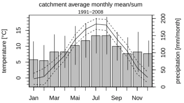
catchment average monthly mean/sum 1991−2008
Fig. 1. Thur catchment average mean monthly temperature (solid
line) and precipitation sum (bars) in the study period 1991–2008. The dashed lines and vertical bars show one standard deviation.
interest. The maximum of runoff in April can be attributed to snowmelt. The runoff minima from September to Febru-ary, depending on the considered quantile, are caused by the combination of less precipitation and snow accumulation.
This catchment, which is relatively large for Alpine con-ditions, was chosen as in smaller catchments streamflow drought rarely occurs over a longer period. In small catch-ments, low streamflow events are easily interrupted by small-scale precipitation events, which complicates the evalua-tion of longer-lasting events. A large catchment is therefore thought to be more appropriate to demonstrate the forecast value for longer events happening within the range of one month. Besides that, the runoff regime is relatively unaf-fected by human influences; i.e., no reservoirs or weirs are installed (Gurtz et al., 1999) that could potentially alter the runoff during periods of low streamflow.
2.2 Meteorological forcing
The unified variable resolution ensemble prediction system VarEPS (Vitart et al., 2008a,b) operated by the ECMWF pro-duces each week a global, 51-member forecast with a lead time of 32 days. Its horizontal resolution is 50 km for the first 10 days and 80 km in the remaining 11–32 days. From day 10 onwards, the atmospheric model is coupled to an oceanic model. The motivation for varying the resolution is to ben-efit from the higher resolution in the early forecast range at longer lead times. At the time of this study, the forecasts were issued for Thursday at 00:00 UTC and were archived in time-steps of 6 h.
With each run of the operational VarEPS, an ensemble re-forecast is started for the same day of the year over the past 18 yr, and also ranges over 32 days. The reforecasts share the same model version as the forecasts and are meant to capture the same model errors, e.g., to allow for an efficient post-processing, a more robust evaluation of forecast skill and a more target-oriented model development. The VarEPS reforecast dataset consists of 954 (18 yr×53 initializations
per year) ensemble forecasts. Unlike the operational forecast, the reforecasts have 5 ensemble members only, initialized with states taken from the ECMWF global reanalysis ERA-Interim or from ERA40. More detailed information about the history of model developments is available at http://www. ecmwf.int/products/data/technical/model id/index.html.
For this study the VarEPS 5-member reforecast is used to drive the hydrological model. Fields of wind speed, 2 m tem-perature, 2 m dew point, sunshine duration, surface albedo and solar radiation are required as input. To meet the grid size of the hydrological model of 500 m×500 m, a down-scaling was performed, based on a bilinear interpolation (Gurtz et al., 1999; Viviroli and Gurtz, 2007). Temperature was adjusted according to elevation, assuming a lapse rate of 0.65◦C/100 m (Jaun and Ahrens, 2009).
2.3 Hydrological model
Runoff predictions were generated using the semi-distributed hydrological model Precipitation Runoff EVApotranspira-tion Hydrotope (PREVAH, Viviroli et al., 2009), with VarEPS as the meteorological forcing. PREVAH consists of hydrological response units (HRUs) and a runoff generation module based on the HBV model (Bergstr¨om and Forsman, 1973), taking account of the spatial distribution. Informa-tion on PREVAH physics and the parameterizaInforma-tion is given in Gurtz et al. (1999) and Viviroli and Gurtz (2007). PRE-VAH’s parameter setting was conditioned by matching the produced runoff to observed runoff at the gauging station in Andelfingen for the period from 1995–2000. This optimiza-tion was performed with a focus on the average flow volume. PREVAH runs in hourly time steps. For this study, however, only daily mean runoff is considered. The setup of PREVAH adopted for the Thur basin is the same as the one used in Fun-del and Zappa (2011) and Zappa and Kan (2007). In the latter publications the calibration and verification of the modeled runoff against the observed runoff, the water balance compo-nents, and hydrographs are presented.
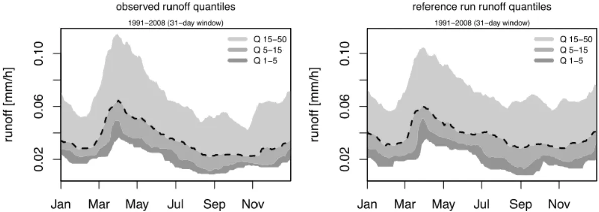
Initial conditions for each forecast run were obtained from a continuous reference simulation forced with meteorologi-cal surface observations from 12 measurement sites, 6 within and 6 outside a distance of 100 km to catchment. The ini-tial states contain information about the water storage in the different modules of each HRU. To highlight the quality of the initial conditions, Fig. 2 shows a comparison of the ref-erence simulation and the runoff observed at the gauging station in Andelfingen for the low runoff regime. The sea-sonal cycle and the runoff volume concur well. The evalua-tion of daily mean runoff from the reference simulaevalua-tion dur-ing the study period 1991–2008 results in a mean error of
−0.003 mm h−1(−3 %), a Nash–Sutcliffe coefficient (Nash and Sutcliffe, 1970) of 0.87 respectively 0.88 using logarith-mized runoff.
Jan Mar May Jul Sep Nov
0.02
0.06
0.10
runoff [mm/h]
Q 15−50 Q 5−15 Q 1−5 observed runoff quantiles
1991−2008 (31−day window)
Jan Mar May Jul Sep Nov
0.02
0.06
0.10
runoff [mm/h]
Q 15−50 Q 5−15 Q 1−5 reference run runoff quantiles
1991−2008 (31−day window)
Fig. 2. Lower runoff quantiles for the Thur catchment from gauge measurements (left) and the hydrological reference run (right). The
quantiles were calculated for daily mean runoff and non-exceedance probabilities of 1 %, 5 %, 15 % (dashed line) and 50 %, utilizing a window of 31 days around the day of interest.
several days, is often applied to the data in order to avoid counting several short events that belong to the same larger-scale drought. Here, however, no further smoothing of the daily forecasts is applied, mainly in order to evaluate the pre-dictive capability of the hydrometeorological prediction sys-tem that has the potential to simulate short-term variability in runoff but also due to the fact that shorter events of abnor-mally low streamflow can lead to economic losses as well.
2.4 Characterization of hydrological droughts
Streamflow droughts are generally characterized by the in-dices duration (time between onset and offset), severity (cu-mulative water deficit) and magnitude (severity/duration) (Tallaksen et al., 1997; Hisdal and Tallaksen, 2000; Hisdal et al., 2001; Smakhtin, 2001; Zaidman et al., 2002; Fleig et al., 2006; Nalbantis and Tsakiris, 2008; Mishra and Singh, 2010; Yoo et al., 2011). Defining hydrological droughts solely by considering those indices requires the assignment of a runoff threshold. Whenever the predicted or observed runoff falls below that threshold, this counts as an event of streamflow drought. Figure 3 illustrates the streamflow drought indices drawn from an observed or forecast hydro-graph, with indices being dependent on the choice of the threshold. It is, however, not obvious where the threshold should be set. Some stakeholders sensitive to low streamflow may be interested in a constant threshold, e.g., a power plant that requires a certain amount of water for cooling. Others might be affected by droughts only in certain seasons, e.g., tourism. To meet both concerns, a variable, quantile-based streamflow drought threshold was selected. The threshold was calculated individually for each day of the year, using runoff from the 18-yr study period and a gliding 31-day win-dow around the date of interest. This implicates that events are classified as streamflow drought in parts of the year as-sociated with higher runoff, which would not be considered as streamflow drought events in other, drier parts of the year. However, in this study streamflow drought is interpreted as
ru
n
o
ff
lead-time
low-flow threshold
duration
severity
timing
initialization day 32
Fig. 3. Illustration of the streamflow drought indices considered in
this study. The solid line is the observed or forecast runoff, i.e., in certain periods, above or below the streamflow drought detection threshold (dashed line). For each forecast member of each 32-day forecast and the corresponding observation, the longest consecutive period below the threshold (streamflow drought duration) is eval-uated. The water deficit during this period (severity, shaded area) is the cumulative difference between the threshold and runoff. The quotient of severity and duration, called magnitude, is evaluated as well. Timing is defined as the moment when half of the event has happened.
exceptionally low with respect to what is expected in a cer-tain part of the year. The actual quantile chosen for the vary-ing threshold is selected later, based on the quality of the forecasts of derived streamflow drought indices and the ro-bustness of the results.
verification results of streamflow drought duration. Possible nonlinearities in the prediction bias could, however, influ-ence the verification results of streamflow drought severity and magnitude. Besides that, the forecast error could vary with lead time. Therefore, a lead time dependency of the streamflow drought threshold was implemented by deriving the threshold from a climatology of forecasts stratified by its lead time. After all, a bias could be removed by, e.g., statis-tical post-processing. However, well-calibrated forecasts of rare events require a large training dataset, which is why this simple method is preferred.
Within the 32-day forecast range, the events of observed or forecast runoff falling below the streamflow drought thresh-old were detected and the streamflow drought indices were calculated. In addition to that, the timing of each streamflow drought event was calculated as the center time between on-set and end of an event. If more than one event was detected within a forecast interval of 32 days, the longest consecu-tive period of low streamflow was considered as the fore-cast/observed event. Forecast and observed events do not necessarily have to overlap, neither between forecast and ob-servation nor between the ensemble forecast members. The forecast system is reduced with the objective to answer the following questions: what is the longest expected stream-flow drought event within the next 32 days and was such an event observed? In the case of probabilistic forecasts, the question is different: what is the probability of exceeding a streamflow drought event ofxdays duration (ymm severity; y/xmm day−1magnitude) within the next 32 days? By do-ing so, an imprecise timdo-ing of the forecast low streamflow event does result in a less strong degradation of the verifica-tion score. For events truncated by the limited forecast range of 32 days, an influence on the verification score caused by deficiencies in forecast timing cannot be excluded. In the here used forecast data, 29 % of the events are still prevalent at the end of the forecast range at day 32.
Duration, severity and magnitude of streamflow droughts are clearly not independent as they are all calculated from the same set of events. For example an event of long duration is likely to be very severe as well. Their forecast performances are therefore expected to be similar. Still, the different in-dices should reflect the demands of different interest groups to a streamflow drought forecast. For hydro-power produc-tion, for example, the severity might be of paramount in-terest, whereas for power-plant cooling the duration is more crucial.
2.5 Verification scores
The focus of the verification of ensemble streamflow drought index forecasts is set on the value they have for potential forecast users. A score, designed to give the value of a fore-cast depending on the vulnerability of a forefore-cast user to a certain event, is the relative value or value score (Murphy, 1977; Richardson, 2000; Roulin, 2007). The user is supposed
to take preventive action whenever a forecast is issued with a probability exceeding the user’s personal cost-loss ratio. Loss is the customers expense when being struck by an event with-out any preparation. Cost is what the user would spend on taking preventive action. The value score then gives the rel-ative economic gain for the user when following the advice of the forecast, compared to having only the climatological event frequency as a basis for decision-making. The value score varies between≤0 (no additional forecast value) and 1 (perfect forecast). Note that even if the value score equals 1, the user still has to bear the costs for taking preventive ac-tion. The value score is calculated for probabilistic forecasts of exceeding a threshold. It gives a value for each possible probability the prediction system can issue, depending on the cost-loss ratio. The upper envelope of all value curves gives the value of the prediction system.
Another score, designed to give an intuitive measure of the prediction system performance, is the generalized discrimi-nation score, or two alternatives forced choice score (2AFC) (Mason and Weigel, 2009; Weigel and Mason, 2011). The score is based on pairs of observations and forecasts. It re-flects the forecast performance in discriminating between different observations. An appealing property of the score is its applicability for ensemble, probabilistic, dichotomous, polychotomous or continuous forecasts and corresponding observations. Here, as an illustration, we give the formula-tion for probabilistic forecast; for all other possible combi-nations of forecast and observation type, referred to Mason and Weigel (2009) and Weigel and Mason (2011). Letn1be
the number of observed eventsi,n0the number of nonevents j. With p1,j respectively p0,i as forecast probabilities for
events that respectively did not occur, the 2AFC score is cal-culated as
2AFC= 1 n0n1
n0
X
i=1
n1
X
j=1
I p0,i, p1,j
(1)
applying the rule
I p0,i, p1,j
=
0.0 if p1,j< p0,i
0.5 if p1,j=p0,i
1.0 ifp1,j> p0,i.
(2)
5 10 15 20 25 30
0.2
0.4
0.6
0.8
lead−time [d]
quantile
2AFC score 1991−2008
0.5 0.6 0.7 0.8 0.9 1.0
5 10 15 20 25 30
0.2
0.4
0.6
0.8
lead−time [d]
quantile
maximum relative value score 1991−2008
0.0 0.2 0.4 0.6 0.8 1.0
a) b)
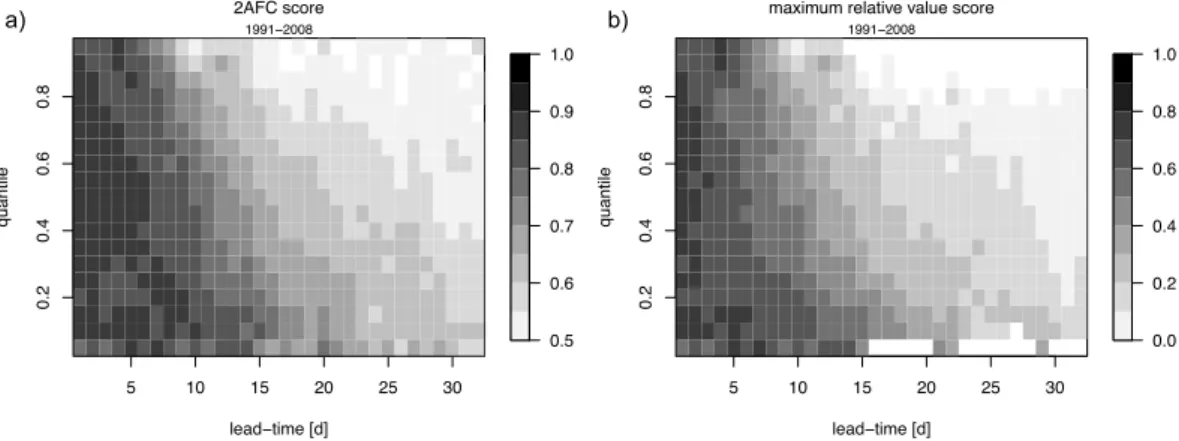
Fig. 4. 2AFC and maximum relative value scores for the Thur VarEPS/PREVAH daily mean runoff forecasts up to a lead time of 32 days. In
the study period 1991–2008, probabilities of the ensemble forecasts to exceed different, quantile-based, varying thresholds are verified.
3 Results
In this section, the forecast quality for different flow regimes is evaluated on a daily basis as well as for scenarios described by the streamflow drought indices. This comprises the choice of a daily varying streamflow drought detection threshold and the assessment of the quality and impact of the initial conditions. The economic value of streamflow drought index forecasts is given for different interest groups.
3.1 Extended lead-time forecast quality
One basic hypothesis of this study is the better predictability of low streamflow events than peak-flow events. As a conse-quence, longer range forecasts of streamflow droughts should prove useful for end users. To back up this hypothesis, it is tested how well the forecast system can predict the proba-bility to exceed different thresholds, from very low to very high runoff, depending on the forecast lead time. A number of ascending quantiles from the complete gauged Thur runoff time series available are used as thresholds. The thresholds are, as described in Sect. 2.4, calculated on a daily basis. Some of the lower quantiles can be seen in Fig. 2. Figure 4a shows the 2AFC score for forecast probabilities to exceed these thresholds for lead times from 1 to 32 days. The results support the hypothesis. Peak flow forecasts, i.e., exceedance probabilities for the 80th quantile and above, show very lit-tle to no skill past about day 15. In contrast, probabilistic low streamflow forecasts, e.g., for the 20th quantile, are skil-ful up to the end of the forecast range. At low thresholds, the forecast quality decreases less rapidly with growing lead time. A very similar picture is obtained when using the rela-tive value score. Figure 4b shows the maximum of this score for any cost/loss ratio. Peak-flow forecasts show no relative value past a lead time of 15 days, whereas probabilistic fore-casts of low streamflow are valuable over the entire forecast range. Relative values greater than 0.6 are possible up to a lead time of 15 days and more than 0.1 at 32 days. For both
plots in Fig. 4, not significantly skilful score values are col-ored white. This was tested by resampling the underlying verification data 1000 times with replacement and applying a t-test with a confidence level of 0.95 to see whether the score mean was significantly larger than the smallest value considered as skilful.
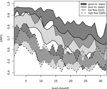
The long-term predictability of streamflow drought events might be attributed to the persistence of the initial state of the model. Conceptually, the recession rate of streamflow is a function of the streamflow itself (e.g., Kirchner, 2009). The lower the streamflow, the slower any further reduc-tion occurs. Consequently, a good initializareduc-tion of the pre-diction model is especially crucial for forecasts of stream-flow drought events. If the initialization leads to a surplus of runoff, for example, the streamflow drought threshold might not be crossed within the forecast range or, at least, the fore-cast timing would be poor.
5 10 15 20 25 30
0.4
0.5
0.6
0.7
0.8
0.9
1.0
lead−time[d]
2AFC
good ini. states poor ini. states low flow (Q15) high flow (Q85)
Fig. 5. 2AFC scores of probabilistic VarEPS/PREVAH daily runoff
forecasts for different lead time ranges, different exceedance thresh-olds and different initial states qualities. The polygons show the 90 % confidence interval, found by resampling 1000 times.
forecast of higher runoff is lost after about one week. This illustrates the importance of a good initialization, especially in the context of forecasting streamflow drought events.
3.2 Choice of the streamflow drought detection threshold
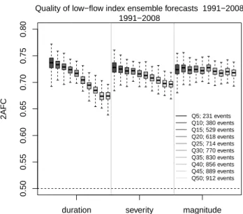
To proceed from forecasts of daily runoff to forecasts of streamflow drought indices, a threshold needs to be selected. Therefore, the performance of low streamflow index ensem-ble predictions, according to the choice of thresholds used to define a streamflow drought event, is evaluated next. The result of this analysis should give an indication about which threshold would be most appropriate for the subsequent ver-ification of the streamflow drought index forecasts. Figure 6 shows the verification results of ensemble duration, sever-ity and magnitude forecasts for streamflow drought detec-tion thresholds from the varying 5th to 50th quantile of Thur runoff. The boxes indicate the range and inter-quartile range found by 1000 times random resampling of the dataset. For all indices, the overall forecast performance appears to be better if a lower threshold is chosen. Duration forecasts de-grade most strongly with higher thresholds, but stay skilful with a 2AFC score of 67 % when using the 50th quantile. Severity forecasts reach a 2AFC score of about 70 % for the 50th quantile, and the magnitude forecast skill stays constant at about 72 % within the uncertainty bounds when varying the threshold. The decrease in forecast skill with increas-ing threshold can be attributed to the enlarged uncertainty in the forecast itself. The higher uncertainty about the score at lower thresholds is a result of the lower number of events. For the subsequent evaluation of streamflow drought index
forecasts, a threshold based on the varying 15th quantile is applied, resulting in 529 events detected for 954 ensemble forecasts (Fig. 6). The choice of the 15th quantile is a com-promise between the number of streamflow drought events and the significance of the findings regarding low stream-flow. The runoff associated with the 15th quantile, i.e., the streamflow drought detection threshold used for our research catchment, can be deduced from Fig. 2. A distinct seasonal runoff maximum occurs in April due to the contribution of snowmelt. The yearly minimum is reached in October or November, when snow accumulation starts.
3.3 Streamflow drought indices prediction/observation
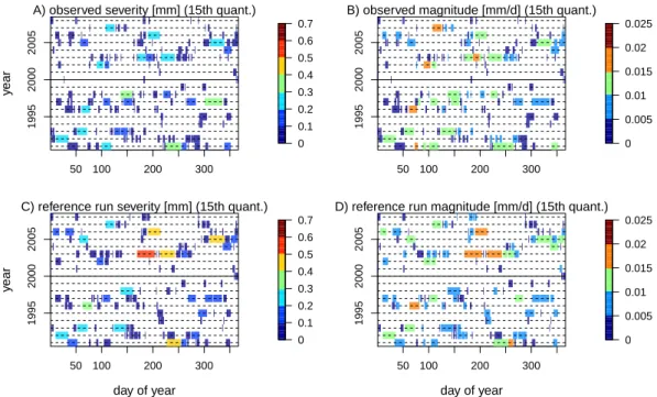
As already shown, the quality of a streamflow drought fore-cast relies greatly on the quality of the representation of the catchment initial state in the hydrological model. This initial state is taken from a reference run, forced with meteorolog-ical surface observation. Usually, without having measure-ments of the state variables of hydrological models avail-able, one way to infer the quality of the initial state is to look at a good reproduction of runoff by the reference run. Figure 7 shows the occurrence (therefore indirectly the du-ration), severity and magnitude of streamflow drought events at the runoff gauge in Andelfingen during the study period 1991 to 2009, as observed or predicted by the reference run. As a streamflow drought detection threshold of varying quan-tiles is used, the events are distributed evenly over the year. The most severe events and the events of greater magnitude however mostly occur in late spring/early summer, when the runoff reaches the yearly maximum due to the contribution of melting snow. The high quality of the reference run already mentioned is also reflected in its representation of the stream-flow drought indices. A high degree of agreement between observation and reference can be seen in the occurrence and timing of the events. High severities and magnitudes in the observations are also strong events in the reference run, al-though the absolute number can vary. Altogether, the initial states seem to provide a reasonable basis for the initialization of forecasts.
2AFC
duration severity magnitude
0.50
0.55
0.60
0.65
0.70
0.75
0.80
Quality of low−flow index ensemble forecasts 1991−2008 1991−2008
Q5; 231 events Q10; 380 events Q15; 529 events Q20; 618 events Q25; 714 events Q30; 770 events Q35; 830 events Q40; 856 events Q45; 889 events Q50; 912 events
Fig. 6. Overall performance of duration, severity and magnitude
ensemble forecasts, subject to the chosen streamflow drought de-tection threshold for the Thur catchment. The boxes indicate the range, inter-quartile range and median of the 2AFC score, found by resampling the forecast in the verification period 1000 times. The number of observed streamflow drought events for each threshold is given in the legend.
forecasts such an event can exceed the forecast range, or a forecast might start during an event. As in observation and reference run, the occurrence of streamflow drought events is distributed equally over the year in the forecasts, which was expected as the detection threshold varies with season. One noticeable feature that can be seen in the ensemble forecasts and the observations is the distinct signal left by the 2003 drought caused by a heat wave that affected large parts of Europe (Beniston, 2004; Sch¨ar et al., 2004; Zappa and Kan, 2007).
The first impression of over-forecasting is confirmed by the rank histograms (Talagrand et al., 1997) in Fig. 9. A dis-proportionately large part of observations fall in the lower bins spanned by the ensemble members. This lack of relia-bility is most distinct for magnitude forecasts, and less for forecasts of duration and severity. However, the discrepancy between the forecast probability and the observed frequency is a type of error that could possibly be corrected for with a statistical post-processing. Such a model bias was partly corrected for by using separate detection thresholds for ob-servations and for forecasts.
3.4 Relative economic value
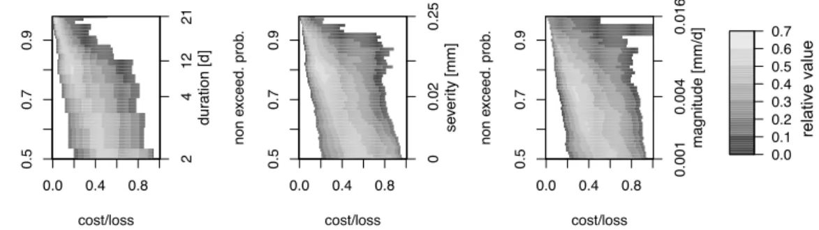
The economic value of probabilistic forecasts of stream-flow droughts, exceeding different levels of duration, severity and magnitude was calculated for forecast probabilities us-ing the 15th quantile streamflow drought detection threshold (Fig. 10). Value scores>0 are shown for a variety of forecast
users, characterized by their individual cost-loss ratio. It ap-pears that, for all thresholds and indices, valuable forecasts for certain user groups can be produced. Especially risk-averse forecast users with low cost-loss ratios would ben-efit from ensemble forecasts for events of long duration or high magnitude and severity. In contrast, forecasts of longer, more severe events have no additional value for users with higher cost-loss ratios. These users would benefit from prob-abilistic forecasts of less intense events. For all users with cost/loss ratios <0.6, i.e., especially the risk-averse users, value scores>50 % are possible. The same evaluation was performed for streamflow drought index forecasts using a higher or lower streamflow drought detection threshold (not shown). In accordance with Fig. 6, higher value scores are possible with the 5th quantile, and lower scores with the 50th quantile as detection threshold. The highest value score for each threshold is reached where the cost-loss ratio concurs with the climatological frequency of the event. This prop-erty of the value score is the reason for the shift to the left with increasing thresholds. The maximum of the value score, however, is not strongly dependent on the duration, severity or magnitude of the event and is here reaching values of 0.4– 0.6.
A direct comparison of the forecast quality of streamflow drought indices with the quality of probabilistic daily predic-tions as shown in Fig. 4 is not possible, as streamflow drought events typically cover several days and no longer contain in-formation about the lead time. The loss of predictive skill of daily probabilistic forecasts with growing lead time has already been addressed (Fig. 4). In comparison, the maxi-mum value score of probabilistic streamflow drought index forecasts is not strongly dependent on the duration, severity or magnitude of the event . As the timing of the streamflow drought events is not exactly specified, but is somewhere be-tween day 1 and day 32, the value score for the events ranges around the lead time averaged value score of the probabilistic daily forecasts as shown in Fig. 4b.
3.5 Timing
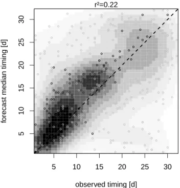
One drawback when forecasting streamflow drought indices instead of the full hydrograph is the lack of information ob-tained about the timing of the event. An approach to evaluate this forecast characteristic is to consider timing as the center time between event onset and end of the event or forecast, as described in Sect. 2.3 or Fig. 3. The median of the ensemble of forecast timings is evaluated against the observed timing. Due to the forecast range, the timing is restricted to 32 days, whereas this limit can only by reached by events starting on the last day of the forecast. A concentration of events will have a timing around 16 days, because the longer the event, the closer the timing has to be to the center of the forecast range.
50 100 200 300
1995
2000
2005
A) observed severity [mm] (15th quant.)
y
ear
0 0.1 0.2 0.3 0.4 0.5 0.6 0.7
50 100 200 300
1995
2000
2005
B) observed magnitude [mm/d] (15th quant.)
0 0.005 0.01 0.015 0.02 0.025
50 100 200 300
1995
2000
2005
C) reference run severity [mm] (15th quant.)
day of year
y
ear
0 0.1 0.2 0.3 0.4 0.5 0.6 0.7
50 100 200 300
1995
2000
2005
D) reference run magnitude [mm/d] (15th quant.)
day of year
0 0.005 0.01 0.015 0.02 0.025
Fig. 7. Periods of streamflow drought occurrence, with severity (A and C) and magnitude (B and D) indicated by colors. (A) and (B) are
derived from the observed runoff, while (C) and (D) are derived from the reference run
1995 2000 2005
0
10
20
30
dur
ation [d]
1995 2000 2005
0.0
0.3
0.6
se
v
er
ity [mm]
1995 2000 2005
0.000
0.015
magnitude [mm/d]
year
Fig. 8. Concatenation of weekly issued ensemble forecasts of streamflow drought duration, severity and magnitude from the 32-day lead
rank
counts
0 2 4
0
100
250
duration
rank
counts
0 2 4
0
100
250
severity
rank
counts
0 2 4
0
100
250
magnitude
Fig. 9. Rank histograms with 90 % confidence intervals of forecast duration, severity and magnitude. The histogram shows the number
of observations attributed to each rank, i.e., the number of times observations lie within the 6 classes formed by the 5-member ensemble forecast. A well-calibrated ensemble prediction system would match the dashed line.
0.0 0.4 0.8
0.5
0.7
0.9
cost/loss
non e
xceed. prob
.
dur
ation [d]
2
4
12
21
0.0 0.4 0.8
0.5
0.7
0.9
cost/loss
non e
xceed. prob
.
se
v
er
ity [mm]
0
0.02
0.25
0.0 0.4 0.8
0.5
0.7
0.9
cost/loss
non e
xceed. prob
.
magnitude [mm/d]
0.001
0.004
0.016
0.0 0.1 0.2 0.3 0.4 0.5 0.6 0.7
re
la
ti
ve
va
lu
e
Fig. 10. Relative economic value of Thur ensemble forecasts of streamflow drought duration, magnitude and severity (columns) using the
varying 15th quantile of runoff as the streamflow drought detection threshold. The economic value is shaded in gray for forecast users with different cost-loss ratios (x-axis) and for different event thresholds. The left y-axis shows the non-exceedance probability and the right y-axis the quantiles for the 50th, 70th, 80th and 95th non-exceedance probability.
cases when a forecast streamflow drought event was ob-served. Of all forecast events, 46 % had a counterpart in the observations (hit rate), and 32 % were missed or false alarms. Figure 11 shows how the timing of the observed event relates to the ensemble median of the predicted timing for the 42 % of hits. The data exhibit a lot of scatter, but, as underlined by the 2-d density map, the forecast timing can explain 22 % of the variance in the observed timing. In order to attribute a forecast event to an observed event, the events should at least for one day overlap. This is the case for 49 % of all hits.
4 Discussion and conclusions
Eighteen years of weekly initialized, hydrological ensem-ble forecasts of daily mean runoff for the Thur catchment in Switzerland, with a lead time of 32 days, were evaluated. The focus was on their potential to provide skilful, and thus valuable, information about the characteristics of streamflow droughts. The basic assumption of a higher predictability of low flow than peak flow was confirmed by the verification results. This was attributed to the fact that long-lived pro-cesses dominate the recession behavior of the runoff. For higher flow, in contrast, the quality of the runoff forecasts is strongly dependent on the correct timing and the amount of
precipitation given by the meteorological forcing model, lim-iting predictability. The positive effect of good initial states on the forecast quality is quickly lost in those cases. This was also confirmed for catchments prone to flash floods, where the influence of initial conditions was found to be already lost after just a few hours (Zappa et al., 2011).
5 10 15 20 25 30 5 10 15 20 25 30
observed timing [d]
forecast median timing [d]
● ● ● ● ● ● ● ● ● ● ● ● ● ● ● ● ● ● ● ● ● ● ● ● ● ● ● ● ● ● ● ● ● ● ● ● ● ● ● ● ● ● ● ● ● ● ● ● ● ● ● ● ● ● ● ● ● ● ● ● ● ● ● ● ● ● ● ● ● ● ● ● ● ● ● ● ● ● ● ● ● ● ● ● ● ● ● ● ● ● ● ● ● ● ● ● ● ● ● ● ● ● ● ● ● ● ● ● ● ● ● ● ● ● ● ● ● ● ● ● ● ● ● ● ● ● ● ● ● ● ● ● ● ● ● ● ● ● ● ● ● ● ● ● ● ● ● ● ● ● ● ● ● ● ● ● ● ● ● ● ● ● ● ● ● ● ● ● ● ● ● ● ● ● ● ● ● ● ● ● ● ● ● ● ● ● ● ● ● ● ● ● ● ● ● ● ● ● ● ● ● ● ● ● ● ● ● ● ● ● ● ● ● ● ● ● ● ● ● ● ● ● ● ● ● ● ● ● ● ● ● ● ● ● ● ● ● ● ● ● ● ● ● ● ● ● ● ● ● ● ● ● ● ● ● ● ● ● ● ● ● ● ● ● ● ● ● ● ● ● ● ● ● ● ● ● ● ● ● ● ● ● ● ● ● ● ● ● ● ● ● ● ● ● ● ● ● ● ● ● ● ● ● ● ● ● ● ● ● ● ● ● ● ● ● ● ● ● ● ● ● ● ● ● ● ● ● ● ● ● ● ● ● ● ● ● ● ● ● ● ● ● ● ● ● ● ● ● ● ● ● ● ● ● ● ● ● ● ● ● ● ● ● ● ● ● ● ● ● ● ● ● ● ● ● ● ● ● ● ● ● ● ● ● ● ● ● ● ● ● ● ● ● ● ● ● ● ● ● ● ● ● ● ● ● ● ● ● ● ● ● ● ● ● ● ● ● ● ● ● ● ● ● ● ● ● ● ● ● ● ● ● ● ● ● ● ● ● ● ● ● ● ● ● ● ● ● ● ● ● ● ● ● ● ● ● ● ● ● ● ● ● ● ● ● ● ● ● ● ● ● ● ● ● ● ● ● ● ● ● ● ● ● ● ● ● ● ● ● ● ● ● ● ● ● ● ● ● ● ● ● ● ● ● ● ● ● ● ● ● ● ● ● ● ● ● ● ● ● ● ● ● ● ● ● ● ● ● ● ● ● ● ● ● ● ● ● ● ● ● ● ● ● ● ● ● ● ● ● ● ● ● ● ● ● ● ● ● ● ● ● ● ● ● ● ● ● ● ● ● ● ● ● ● ● ● ● ● ● ● ● ● ● ● ● ● ● r²=0.22
Fig. 11. Observed vs. forecast lead times (median) of streamflow
drought events. The center between the onset and offset of an event was chosen as the lead time. The background field is the estimated 2-d density (dimensionless). The black dots mark the events that overlap by at least 1 day with the observed event.
Having ensemble forecasts of the streamflow drought in-dices duration, severity and magnitude at hand was shown to provide additional value to end users. Using those fore-casts results in an economic advantage, mostly independent of the duration, severity or magnitude of the event. Compared to daily forecasts, streamflow drought index forecasts are of reduced complexity, as they no longer contain information about the timing of the streamflow drought event. Hence, the forecast system is less penalized when the onset and offset of streamflow drought events are lagged compared to obser-vations, which enhances the value of the forecasts. It was shown that streamflow drought index forecast can reach eco-nomical values greater 50 % for the more risk-averse users. A comparison of the forecast timing of drought events with the observed timing showed that this information gives only a rough estimate. The forecasts of streamflow drought indices can provide useful information about the characteristics of an upcoming event. The timing prediction should, however, be handled with caution.
The ensemble forecasts evaluated in this study were per-formed for a relatively large alpine catchment. This was cho-sen mainly in order to ensure the occurrence of longer peri-ods of low streamflow, as in larger catchments runoff is not as strongly affected by small or local precipitation events. However, we also tested streamflow drought predictions for smaller alpine catchments. There, only shorter stream-flow drought events could be evaluated and the value of
these forecasts was found to be lower. Nevertheless, stream-flow drought index forecasts can still be useful for smaller catchments.
When analyzing streamflow droughts on time scales of one month or longer, it is common to apply a smoothing of the observed or forecast streamflow time series. This should prevent counting shorter streamflow depletions as individual drought events, although they belong to the same larger-scale drought. Such a smoothing is not applied in this study as also short-term water shortages of one day can have an eco-nomical impact, independent on whether the single events are induced by a larger-scale drought event or not. Sectors prone to short-term streamflow droughts are, e.g., shipping, hydro-power production or power production in general as the cooling of many power plants depends on the availability of river water. Forecast users from those sectors could po-tentially benefit from forecast of short events, and this study investigates the potential of a hydrometeorological forecast system to predict them.
Further refinements could improve the predictability of streamflow droughts. The parameters of the hydrological model PREVAH were found by optimizing the predicted runoff subject to average flow volume. This is certainly not the best approach for streamflow drought forecasts and might introduce biases in predictions of the lower flow regime. Our findings, however, suggest that an operationally used hy-drological prediction system, which is meant to give warn-ings primarily of peak flow, can without larger modifications also be suitable for forecasting streamflow droughts. Biases due to inadequate model parameterization can be partly ad-dressed by a simple statistical post-processing, e.g., defin-ing the streamflow drought threshold for the observed runoff from an observation climatology and for forecast runoff from past model predictions. More complex methods could be considered, but this was beyond the scope of this study.
The downscaling of the meteorological model could be further improved. In this study, the relatively coarse horizon-tal grid of the meteorological forcing model was downscaled to the grid of the hydrological model by a simple bilinear in-terpolation. A dynamic downscaling involving one or more nested regional models would be preferable. However, no such approach was available for the region and the forecast range of one month considered here.
Acknowledgements. Support from the Swiss National Research
Program Sustainable Water Management (NRP 61 project DROUGHT-CH) is gratefully acknowledged. We also express our gratitude to ECMWF and MeteoSwiss for providing the necessary data.
Edited by: A. Gelfan
References
Beniston, M.: The 2003 heat wave in Europe: A shape of things to come? An analysis based on Swiss climatological data and model simulations, Geophys. Res. Lett., 31, L02202, doi:10.1029/2003GL018857, 2004.
Bergstr¨om, S. and Forsman, A.: Developement of a conceptual de-terministic rainfall–runoff model, Nord. Hydrol., 4, 147–170, doi:10.2166/nh.1973.012, 1973.
Bordi, I. and Sutera, A.: DROUGHT MONITORING AND FORE-CASTING AT LARGE SCALE, in: Methods and Tools for Drought Analysis and Management, edited by: Rossi, G., Vega, T., and Bonaccorso, B., Chap. 1, 3–27, Springer Netherlands, doi:10.1007/978-1-4020-5924-7 1, 2007.
Cacciamani, C., Morgillo, A., Marchesi, S., and Pavan, V.: Monitor-ing and forecastMonitor-ing drought on a regional scale: Emilia-Romagna region, in: Methods and Tools for Drought Analysis and Man-agement, edited by: Rossi, G., Vega, T., and Bonaccorso, B., Chap. 2, 29–48, Springer Netherlands, doi:10.1007/978-1-4020-5924-7 2, 2007.
Cancelliere, A., Mauro, G. D., Bonaccorso, B., and Rossi, G.: Drought forecasting using the Standardized Precipitation Index, Water Resour. Manag., 21, 801–819, doi:10.1007/s11269-006-9062-y, 2006.
Cebri´an, A. C. and Abaurrea, J.: Risk measures for events with a stochastic duration: an application to drought analysis, Stoch. Env. Res. Risk A., 26, 971–981, doi:10.1007/s00477-011-0521-5, 2011.
Chung, C.-H. and Salas, J. D.: Drought Occurrence Probabilities and Risks of Dependent Hydrologic Processes, J. Hydrol. Eng., 5, 259–268, doi:10.1061/(ASCE)1084-0699(2000)5:3(259), 2000.
Cloke, H. L. and Pappenberger, F.: Ensemble flood forecasting: A review, J. Hydrol., 375, 613–626, doi:10.1016/j.jhydrol.2009.06.005, 2009.
Fleig, A. K., Tallaksen, L. M., Hisdal, H., and Demuth, S.: A global evaluation of streamflow drought characteristics, Hydrol. Earth Syst. Sci., 10, 535–552, doi:10.5194/hess-10-535-2006, 2006. Fleig, A. K., Tallaksen, L. M., Hisdal, H., and Hannah, D. M.:
Re-gional hydrological drought in north-western Europe: linking a new Regional Drought Area Index with weather types, Hydrol. Process., 25, 1163–1179, doi:10.1002/hyp.7644, 2011.
Fundel, F. and Zappa, M.: Hydrological Ensemble Forecast-ing in Mesoscale Catchments: Sensitivity to Initial Condi-tions and Value of Reforecasts, Water Resour. Res., 47, 1–15, doi:10.1029/2010WR009996, 2011.
Gurtz, J., Baltensweiler, A., and Lang, H.: Spatially distributed hydrotope-based modelling of evapotran-spiration and runoff in mountainous basins, Hydrol. Process., 13, 2751–2768,
doi:10.1002/(SICI)1099-1085(19991215)13:17<2751::AIDHYP897>3.3.CO;2-F, 1999.
Heim Jr., R. R.: A Review of Twentieth-Century Drought Indices Used in the United States, B. Am. Meteorol. Soc., 83, 1149– 1165, 2002.
Hirschberg, P. A., Abrams, E., Bleistein, A., Bua, W., Monache, L. D., Dulong, T. W., Gaynor, J. E., Glahn, B., Hamill, T. M., Hansen, J. A., Hilderbrand, D. C., Hoffman, R. N., Morrow, B. H., Philips, B., Sokich, J., and Stuart, N.: A Weather and Climate Enterprise Strategic Implementation Plan for Generat-ing and CommunicatGenerat-ing Forecast Uncertainty Information, B. Am. Meteorol. Soc., 92, 1651–1666, doi:10.1175/BAMS-D-11-00073.1, 2011.
Hisdal, H. and Tallaksen, L. M.: Technical Report to the ARIDE project No. 6 Drought Event Definition, Tech. Rep. 6, University of Oslo, 2000.
Hisdal, H., Stahl, K., Tallaksen, L. M., and Demuth, S.: Have streamflow droughts in Europe become more severe or frequent?, Int. J. Climatol., 21, 317–333, doi:10.1002/joc.619, 2001. Hwang, Y. and Carbone, G. J.: Ensemble Forecasts of
Drought Indices Using a Conditional Residual Resam-pling Technique, J. Appl. Meteorol. Clim., 48, 1289–1301, doi:10.1175/2009JAMC2071.1, 2009.
Jaun, S. and Ahrens, B.: Evaluation of a probabilistic hydromete-orological forecast system, Hydrol. Earth Syst. Sci., 13, 1031– 1043, doi:10.5194/hess-13-1031-2009, 2009.
Kim, T.-W. and Vald´es, J. B.: Nonlinear Model for Drought Forecasting Based on a Conjunction of Wavelet Trans-forms and Neural Networks, J. Hydrol. Eng., 8, 319–328, doi:10.1061/(ASCE)1084-0699(2003)8:6(319), 2003.
Kirchner, J. W.: Catchments as simple dynamical systems: Catchment characterization, rainfall-runoff modeling, and do-ing hydrology backward, Water Resour. Res., 45, 1–34, doi:10.1029/2008WR006912, 2009.
Li, H., Luo, L., and Wood, E. F.: Seasonal hydrologic predictions of low-flow conditions over eastern USA during the 2007 drought, Atmos. Sci. Lett., 9, 61–66, doi:10.1002/asl.182, 2008. Lohani, V. K. and Loganathan, G. V.: An early warning
sys-tem for drought management using the palmer drought index, J. Am. Water Resour. As., 33, 1375–1386, doi:10.1111/j.1752-1688.1997.tb03560.x, 1997.
Luo, L. and Wood, E. F.: Monitoring and predicting the 2007 U.S. drought, Geophys. Res. Lett., 34, 1–6, doi:10.1029/2007GL031673, 2007.
Mason, S. J. and Weigel, A. P.: A Generic Forecast Verification Framework for Administrative Purposes, Mon. Weather Rev., 137, 331–349, doi:10.1175/2008MWR2553.1, 2009.
Mishra, A. K. and Desai, V. R.: Drought forecasting using stochastic models, Stoch. Env. Res. Risk A., 19, 326–339, doi:10.1007/s00477-005-0238-4, 2005.
Mishra, A. K. and Desai, V.: Drought forecasting using feed-forward recursive neural network, Ecol. Modell., 198, 127–138, doi:10.1016/j.ecolmodel.2006.04.017, 2006.
Mishra, A. K. and Singh, V. P.: A review of drought concepts, J. Hy-drol., 391, 202–216, doi:10.1016/j.jhydrol.2010.07.012, 2010. Moreira, E., Coelho, C., Paulo, A., Pereira, L., and Mexia, J.:
Morid, S., Smakhtin, V., and Bagherzadeh, K.: Drought forecast-ing usforecast-ing artificial neural networks and time series of drought indices, Int. J. Climatol., 27, 2103–2111, doi:10.1002/joc.1498, 2007.
Murphy, A. H.: The Value of Climatological, Categorical and Probabilistic Forecasts in the Cost-Loss Ratio Situa-tion, Mon. Weather Rev., 105, 803–816, doi:10.1175/1520-0493(1977)105<0803:TVOCCA>2.0.CO;2, 1977.
Nalbantis, I. and Tsakiris, G.: Assessment of Hydrological Drought Revisited, Water Resour. Manag., 23, 881–897, doi:10.1007/s11269-008-9305-1, 2008.
Nash, J. and Sutcliffe, J.: River flow forecasting through conceptual models Part I – A discussion of principles, J. Hydrol., 10, 282– 290, doi:10.1016/0022-1694(70)90255-6, 1970.
¨
Ozger, M., Mishra, A. K., and Singh, V. P.: Long Lead Time Drought Forecasting Using a Wavelet and Fuzzy Logic Combi-nation Model: A Case Study in Texas, J. Hydrometeorol., 13, 284–297, doi:10.1175/JHM-D-10-05007.1, 2012.
Richardson, D. S.: Skill and relative economic value of the ECMWF ensemble prediction system, Q. J. Roy. Meteor. Soc., 126, 649– 667, doi:10.1002/qj.49712656313, 2000.
Rings, J., Vrugt, J. A., Schoups, G., Huisman, J. A., and Vereecken, H.: Bayesian model averaging using particle fil-tering and Gaussian mixture modeling: Theory, concepts, and simulation experiments, Water Resour. Res., 48, W05520, doi:10.1029/2011WR011607, 2012.
Roulin, E.: Skill and relative economic value of medium-range hy-drological ensemble predictions, Hydrol. Earth Syst. Sci., 11, 725–737, doi:10.5194/hess-11-725-2007, 2007.
Sch¨ar, C., Vidale, P. L., L¨uthi, D., Frei, C., H¨aberli, C., Liniger, M. A., and Appenzeller, C.: The role of increasing temperature variability in European summer heatwaves, Nature, 427, 332– 336, doi:10.1038/nature02300, 2004.
Shukla, S. and Lettenmaier, D. P.: Seasonal hydrologic predic-tion in the United States: understanding the role of initial hy-drologic conditions and seasonal climate forecast skill, Hy-drol. Earth Syst. Sci., 15, 3529–3538, doi:10.5194/hess-15-3529-2011, 2011.
Singla, S., C´eron, J.-P., Martin, E., Regimbeau, F., D´equ´e, M., Ha-bets, F., and Vidal, J.-P.: Predictability of soil moisture and river flows over France for the spring season, Hydrol. Earth Syst. Sci., 16, 201–216, doi:10.5194/hess-16-201-2012, 2012.
Smakhtin, V.: Low flow hydrology: a review, J. Hydrol., 240, 147– 186, doi:10.1016/S0022-1694(00)00340-1, 2001.
Steinemann, A. C.: Using Climate Forecasts for Drought Management, J. Appl. Meteorol. Clim., 45, 1353–1361, doi:10.1175/JAM2401.1, 2006.
Tadesse, T., Wilhite, D. A., Hayes, M. J., Harms, S. K., and Goddard, S.: Discovering Associations between Climatic and Oceanic Parameters to Monitor Drought in Nebraska Using Data-Mining Techniques, J. Climate, 18, 1541–1550, doi:10.1175/JCLI3346.1, 2005.
Talagrand, O., Vautard, R., and Strauss, B.: Evaluation of proba-bilistic prediction systems, in: Proc. ECMWF Workshop on Pre-dictability, 1–25, ECMWF, Reading, Berkshire RG2 9AX, UK, 1997.
Tallaksen, L. M., Madsen, H., and Clausen, B.: On the definition and modelling of streamflow drought duration and deficit volume, Hydrolog. Sci. J., 42, 15–33, doi:10.1080/02626669709492003,
1997.
van Ogtrop, F. F., Vervoort, R. W., Heller, G. Z., Stasinopou-los, D. M., and Rigby, R. A.: Long-range forecasting of in-termittent streamflow, Hydrol. Earth Syst. Sci., 15, 3343–3354, doi:10.5194/hess-15-3343-2011, 2011.
Vidal, J.-P., Martin, E., Franchist´eguy, L., Habets, F., Soubeyroux, J.-M., Blanchard, M., and Baillon, M.: Multilevel and multiscale drought reanalysis over France with the Safran-Isba-Modcou hy-drometeorological suite, Hydrol. Earth Syst. Sci., 14, 459–478, doi:10.5194/hess-14-459-2010, 2010.
Vitart, F., Bonet, A., Alonso Balmaseda, M., Balsamo, G., Bidlot, J.-R., Buizza, R., Fuentes, M., Hofstadler, A., Molteni, F., and Palmer, T. N.: Merging VarEPS with the monthly forecasting sys-tem: a first step towards seamless prediction, ECMWF Newslet-ter, 115, 35–44, 2008a.
Vitart, F., Buizza, R., Alonso Balmaseda, M., Balsamo, G., Bidlot, J.-R., Bonet, A., Fuentes, M., Hofstadler, A., Molteni, F., and Palmer, T. N.: The new VarEPS-monthly forecasting system: A first step towards seamless prediction, Q. J. Roy. Meteorol. Soc., 134, 1789–1799, doi:10.1002/qj.322, 2008b.
Viviroli, D. and Gurtz, J.: The Hydrological Modelling System Part II – Physical Model Description, Tech. rep., Institute of Geog-raphy, University of Berne, Geographica Bernensia P40, Berne, 2007.
Viviroli, D., Zappa, M., Gurtz, J., and Weingartner, R.: An introduc-tion to the hydrological modelling system PREVAH and its pre-and post-processing-tools, Environ. Modell. Softw., 24, 1209– 1222, doi:10.1016/j.envsoft.2009.04.001, 2009.
Webster, P. J., Jian, J., Hopson, T. M., Hoyos, C. D., Agudelo, P. A., Chang, H.-R., Curry, J. A., Grossman, R. L., Palmer, T. N., and Subbiah, A. R.: Extended-Range Probabilistic Forecasts of Ganges and Brahmaputra Floods in Bangladesh, B. Am. Meteo-rol. Soc., 91, 1493–1514, doi:10.1175/2010BAMS2911.1, 2010. Weigel, A. P. and Mason, S. J.: The Generalized Discrimination Score for Ensemble Forecasts, Mon. Weather Rev., 139, 3069– 3074, doi:10.1175/MWR-D-10-05069.1, 2011.
Weigel, A. P., Liniger, M. A., and Appenzeller, C.: The Discrete Brier and Ranked Probability Skill Scores, Mon. Weather Rev., 135, 118–124, doi:10.1175/MWR3280.1, 2007.
Wood, A. W., Maurer, E. P., Kumar, A., and Lettenmaier, D. P.: Long-range experimental hydrologic forecasting for the eastern United States, J. Geophys. Res., 107, 1–15, doi:10.1029/2001JD000659, 2002.
Yoo, J., Kwon, H.-H., Kim, T.-W., and Ahn, J.-H.: Drought frequency analysis using cluster analysis and bivariate probability distribution, J. Hydrol., 420–421, 102–111, doi:10.1016/j.jhydrol.2011.11.046, 2011.
Zaidman, M. D., Rees, H. G., and Young, A. R.: Spatio-temporal development of streamflow droughts in north-west Europe, Hy-drol. Earth Syst. Sci., 6, 733–751, doi:10.5194/hess-6-733-2002, 2002.
Zappa, M. and Kan, C.: Extreme heat and runoff extremes in the Swiss Alps, Nat. Hazards Earth Syst. Sci., 7, 375–389, doi:10.5194/nhess-7-375-2007, 2007.