www.atmos-chem-phys.net/13/12481/2013/ doi:10.5194/acp-13-12481-2013
© Author(s) 2013. CC Attribution 3.0 License.
Atmospheric
Chemistry
and Physics
Airborne observations and modeling of springtime
stratosphere-to-troposphere transport over California
E. L. Yates1, L. T. Iraci1, M. C. Roby2, R. B. Pierce3, M. S. Johnson4, P. J. Reddy5, J. M. Tadi´c1,*, M. Loewenstein1,
and W. Gore1
1Atmospheric Science Branch, NASA Ames Research Center, Moffett Field, CA 94035, USA 2Department of Meteorology, San Jose State University, San Jose, CA 95192-0104, USA 3NOAA/NESDIS Advanced Satellite Products Branch Madison, WI 53706, USA
4Biospheric Science Branch, NASA Ames Research Center, Moffett Field, CA 94035, USA
5Air Pollution Control Division, Colorado Department of Public Health & Environment, Denver, CO 80246, USA *now at: Department of Global Ecology, Carnegie Institution for Science, Stanford, CA 94305, USA
Correspondence to:E. L. Yates ([email protected])
Received: 6 March 2013 – Published in Atmos. Chem. Phys. Discuss.: 18 April 2013
Revised: 22 November 2013 – Accepted: 23 November 2013 – Published: 20 December 2013
Abstract. Stratospheto-troposphere transport (STT) re-sults in air masses of stratospheric origin intruding into the free troposphere. Once in the free troposphere, ozone (O3
)-rich stratospheric air can be transported and mixed with tro-pospheric air masses, contributing to the trotro-pospheric O3
budget. Evidence of STT can be identified based on the dif-ferences in the trace gas composition of the two regions. Be-cause O3is present in such large quantities in the stratosphere
compared to the troposphere, it is frequently used as a tracer for STT events.
This work reports on airborne in situ measurements of O3 and other trace gases during two STT events observed
over California, USA. The first, on 14 May 2012, was as-sociated with a cutoff low, and the second, on 5 June 2012, occurred during a post-trough, building ridge event. In each STT event, airborne measurements identified high O3within
the stratospheric intrusion, which were observed as low as 3 km above sea level. During both events the stratospheric air mass was characterized by elevated O3mixing ratios and
reduced carbon dioxide (CO2)and water vapor. The
repro-ducible observation of reduced CO2within the stratospheric
air mass supports the use of non-conventional tracers as an additional method for detecting STT. A detailed meteorolog-ical analysis of each STT event is presented, and observations are interpreted with the Realtime Air Quality Modeling Sys-tem (RAQMS). The implications of the two STT events are
discussed in terms of the impact on the total tropospheric O3
budget and the impact on air quality and policy-making.
1 Introduction
Transport of stratospheric air into the troposphere, referred to as stratosphere-to-troposphere transport (STT), contributes to and alters the trace gas composition of the troposphere, and as such STT has been extensively studied for over 50 yr (e.g., Danielsen, 1968; Danielsen and Mohnen, 1977; Lamar-que and Hess, 1994; Sprenger et al., 2003; Thompson et al., 2007; Lefohn et al., 2011). Ozone (O3)is present in large
quantities in the stratosphere compared to the troposphere and is commonly used as a tracer for STT. In the free tropo-sphere, air masses of stratospheric origin can be transported and mixed with tropospheric air masses, typically forming filamentary structures, which appear as O3 laminae in O3
profiles detected by ozonesondes, in situ aircraft measure-ments and O3lidar (Zanis et al., 2003; Cooper et al., 2005;
Trickl et al., 2011; Langford et al., 2012). Understanding the dynamic processes that control the tropospheric O3budget is
of importance not only for understanding surface air quality in areas affected by STT, but also because upper tropospheric O3is an important greenhouse gas affecting outgoing
STT events are episodic in nature and vary considerably with latitude and season. In western North America (the end of the Pacific storm track) peak STT occurs during the late winter to late spring (e.g., Sprenger et al., 2003; Stohl et al., 2003; Skerlak et al., 2013), when synoptic-scale and mesoscale processes (e.g., tropopause folds in the vicinity of the polar and subpolar jets, cutoff lows, mesoscale convec-tive complexes) facilitate the tropopause to fold, allowing for stratospheric air masses to be transported downward to the troposphere. Tropopause folds and cutoff lows, which em-phasize the vertical structure (former) and horizontal struc-ture (latter) in which a stratospheric intrusion can occur (Stohl et al., 2003), have been identified as the most impor-tant mechanisms to cause STT and have subsequently been the focus of STT investigations (e.g., Danielsen and Mohnen, 1977; Ebel, 1991; Vaughan et al., 1994; Bonasoni, et al., 2000; Søensen and Nielson, 2001; Lefohn et al., 2011). The frequency and magnitude of STT events are important fac-tors in understanding the possible degree to which they affect surface and free troposphere O3mixing ratios (Lefohn et al.,
2011).
The stratosphere and troposphere are separated by the tropopause. Traditionally the tropopause is defined by the “thermal tropopause”, which is the lowest level at which the temperature lapse rate decreases to 2 K km−1or less and the
averaged lapse rate between this level and any level within 2 km does not exceed 2 K km−1 (WMO, 1986). In the
ex-tratropics the tropopause corresponds well with a surface of constant potential vorticity (PV), allowing for a “dynamical tropopause” definition. Tropopause PV values in literature range from 1.6 to 3.5 potential vorticity units (PVU) with 2 PVU used most often (Stohl et al., 2003). Both of these tropopause definitions are routinely used in forecasting and modeling STT events (e.g., Sprenger et al., 2003; Stohl et al., 2003).
Observations of STT have been reported in long-term data sets from mountain-top O3 sites measuring the free
tropo-sphere (e.g., Bonasoni et al., 2000; Stohl et al., 2000) and from O3profiles measured by aircraft, ozonesondes and O3
lidar (e.g., Zanis et al., 2003; Cooper et al., 2005; Bow-man et al., 2007; Bourqui and Trepainer, 2010; Langford et al., 2012). Identifying STT within the tropospheric boundary layer, especially at near-sea-level surface sites, is challeng-ing. The stratospheric characteristics (high O3, low humidity,
high PV) may be lost by the time this air is entrained into the boundary layer, making STT difficult to diagnose and fore-cast. In addition, the O3mixing ratio within STT events is
expected to be highly variable depending on the stratospheric origin and degree of mixing in the free troposphere. Although evidence of STT at sea-level surface sites has been presented (Chung and Dann, 1985; Langford et al., 2012; Lefohn et al., 2012; Lin et al., 2012), the magnitude of the effects of STT on boundary layer O3mixing ratios is still under debate
(Fiore et al., 2003; Langford et al., 2009; Lefohn et al., 2011; Lin et al., 2012).
The United States Environmental Protection Agency (EPA) sets National Ambient Air Quality Standards (NAAQS) for ground-level O3, which are used to assess air
quality. The 2008 NAAQS for O3 require that the 3 yr
av-erage of the annual fourth-highest daily maximum 8 h mean mixing ratio be less than or equal to 75 ppbv (parts per bil-lion by volume) (US EPA, 2006), with a decision on the pro-posed reduction of the NAAQS O3target to 60–70 ppbv due
in 2014 (US EPA, 2010). The formulation of the NAAQS O3standard relies on the accurate identification of a
repre-sentative background mixing ratio of O3 that would occur
in the United States in the absence of anthropogenic contri-butions. Current background O3mixing ratios are estimated
to be in the range of 15–35 ppbv (Fiore et al., 2003), con-tributing up to 47 % towards the current NAAQS O3target of
75 ppbv. Some studies have reported higher background O3
mixing ratios, particularly in springtime, suggesting that STT has a significant influence on the background O3mixing
ra-tios (Cooper et al., 2005; Hocking et al., 2007; Lefohn et al., 2011; Langford et al., 2012, Lin et al., 2012). If the proposed reduction of NAAQS O3target is approved, the identification
of STT and evidence of its contribution towards background O3mixing ratios will become increasingly important, as the
gap between background O3 and the NAAQS O3 target is
reduced.
The western United States, due to its location at the end of the North Pacific mid-latitude storm track, has been iden-tified as a preferred location for deep STT reaching below 700 mbar (Sprenger and Wernli, 2003). Understanding the boundary conditions coming into the western United States is important for air quality issues. However large areas in the western United States have limited or no O3 data. In
addi-tion, the existing positive vertical gradient for O3, complex
mountainous terrain of the western United States and result-ing mesoscale dynamics further complicate efforts to model O3concentrations.
In this paper, a detailed analysis of two STT events occur-ring duoccur-ring spoccur-ring 2012 over California, USA, is presented. This work reports airborne in situ measurements of O3and
other trace gases, providing supporting evidence towards of the use of a non-traditional stratospheric tracer (carbon diox-ide, CO2), which can be used in conjunction with O3to help
2 Experimental approach
2.1 Airborne instrumentation
In situ measurements of O3vertical profiles were carried out
on board the Alpha Jet research aircraft as part of the Alpha Jet Atmospheric eXperiment (AJAX). The aircraft is based at and operated from NASA Ames Research Center at Mof-fett Field, CA (37.415◦
N, 122.050◦
W). Scientific instru-mentation is housed within one of two externally mounted wing pods, each of which has a maximum payload weight of 136 kg. The aircraft was flown with one instrumented wing pod attached, containing an O3 monitor (described below)
and a CO2 analyzer (Picarro Inc., model G2301-m),
modi-fied for flight installation The aircraft also carries GPS and inertial navigation systems that provide altitude, temperature and position information time-stamped with coordinated uni-versal time (UTC) for each research flight.
Measurements of O3mixing ratios were performed using
a commercial O3monitor (2B Technologies Inc., model 205)
based on ultraviolet (UV) absorption techniques and modi-fied for flight worthiness. The dual-beam instrument uses two detection cells to measure simultaneously the UV light inten-sity differences between O3-scrubbed air and un-scrubbed air
to give precise measurements of O3. The monitor has been
modified by upgrading the pressure sensor and pump to al-low measurements at high altitudes, including a lamp heater to improve the stability of the UV source, and the addition of heaters, temperature controllers and vibration isolators to control the monitor’s physical environment.
The air intake is through Teflon tubing (perfluoroalkoxy polymer, PFA) with a backward-facing inlet positioned on the underside of the instrument wing pod. Air is delivered through a 5 µm PTFE (polytetrafluoroethylene) membrane filter to remove fine particles prior to analysis.
The O3monitor has undergone thorough instrument
test-ing in the laboratory to determine the precision, linearity and overall accuracy. Eight-point calibration tests (ranging from 0 to 300 ppbv) were performed before and after each flight using an O3calibration source (2B Technologies, model 306
referenced to the WMO scale). Calibration settings for the O3
monitor were left at manufacturer default settings, and cor-rections to account for linearity offset and zero offset were applied during data processing. For the flights reported here, the linearity offset was determined to be 1.01 and the zero offset was−2.4 ppbv.
Calibrations in a pressure- and temperature-controlled en-vironmental chamber were performed using the O3
calibra-tion source over the pressure range 200–800 mbar and tem-perature range −15 to +25◦
C, typical pressure and tem-perature ranges observed in the wing-mounted instrument pod during flight. Precision during chamber tests, determined from the standard deviation of O3measurements taken every
10 s, when sampling O3mixing ratios of 50 ppbv over 2 min
duration and during simulated descent profiles, was found
to be 2 ppbv. The zero offset, observed when sampling O3
-scrubbed air during simulated descent profiles, was found to increase linearly by 0.6 ppbv with decreasing chamber pres-sure (typical zero offset of −2.4 ppbv at ground level and −3 ppbv at 200 mbar). Instrument drift estimated based on 1 h of sampling 50 ppbv O3was 1.5 ppbv. Overall uncertainty
of the airborne O3measurements is estimated to be 3.0 ppbv.
In situ O3 measurements, taken every 10 s, were
per-formed over the San Joaquin Valley, CA (SJV) (Castle air-port, Merced: 37.381◦
N, 120.568◦
W), and offshore (RAINS Intersection: 37.169◦
N, 123.235◦
W). Takeoff time from Moffett Field was at 18:00 UTC on 14 May 2012 and 5 June 2012. The aircraft arrived on-station at the SJV site at ∼18:20 UTC (local time is UTC−7 h) on each day and per-formed a descending spiral profile from∼8.8 km to < 0.5 km with a descent rate of∼370 m min−1. A second descending
spiral profile was performed over the offshore location each day starting at∼19:05 UTC. On the 14 May 2013, the profile extended from∼8.5 km to 1.5 km; the aircraft was prevented from flying any lower on this day due to a thick marine stratus layer with a top at 1.5 km. The lowest altitude of the offshore profile on 5 June 2012 was < 0.5 km. Total flight time each day was 100 min.
2.2 RAQMS model description
Global in-line O3 and meteorological forecasts from
RAQMS (Pierce et al., 2007, 2009) are used in conjunction with reverse domain filling (RDF) techniques (Sutton et al., 1994; Fairlie et al., 2007) to provide a large scale context for the interpretation of the airborne observations and to assess the fidelity of the RAQMS O3 forecasts. Forecasts are
ini-tialized with satellite-based O3analyses and are archived at
6 h intervals at a horizontal resolution of 1◦
×1◦
with 35 hy-bridη–θvertical levels extending from the surface to approx-imately 60 km. Stratospheric O3 analyses are constrained
through assimilation of near-real-time (NRT) O3 profiles
from the Microwave Limb Sounder (MLS) (Waters et al., 2006) above 50 mbar and NRT cloud-cleared total column O3retrievals from the Ozone Monitoring Instrument (OMI)
(Levelt et al., 2006). The RAQMS dynamical core is the Uni-versity of Wisconsin (UW) hybrid isentropic–eta coordinate (UW hybrid) model (Zapotocny et al., 1997; Schaack et al., 2004), which uses isentropic coordinates above 380 K and hybrid eta coordinates between 380 K and the surface. The vertical resolution depends on the vertical gradient of po-tential temperature and varies between ∼200 m and 1 km (Pierce et al., 2007). Meteorological forecasts are initialized with operational analyses from the National Centers for En-vironmental Prediction (NCEP) Global Data Assimilation System (GDAS) (Kleist et al., 2009). Six-hour chemical and meteorological forecasts provide chemical and meteorologi-cal input for the RDF meteorologi-calculations. Analyzed O3results are
-123.0 -122.5
-122.0 -121.5
-121.0 -120.5
37.1 37.2 37.3 37.4 37.5 37.6 0 2000 4000 6000 8000 10000
Ozone (ppbv)
20 37 53 70 87 103 120
Longitude (
o)
Latitude (
o )
Altitutde (m)
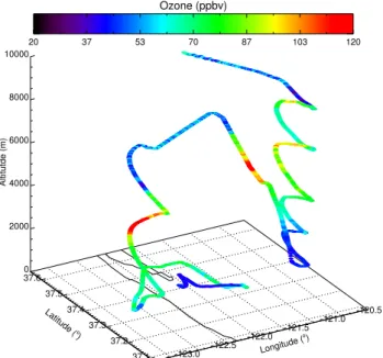
Fig. 1.3-D projection of O3mixing ratio (ppbv) as observed during
flight on 14 May 2012 (takeoff time: 18:00 UTC). The O3monitor
requires a 10 min warm-up period before stable measurements are made, which results in data acquisition starting at 8.4 km during the transit to the San Joaquin Valley (inland) site.
The RDF technique has been shown to represent coarsely resolved constituent fields at higher resolution, with higher information content, than originally observed (Sutton et al., 1994) or modeled (Fairlie et al., 2007). The RAQMS RDF calculations are based on analysis of back trajectories initial-ized along the aircraft flight track. Three-dimensional 6-day back trajectory calculations were conducted using the Lang-ley Trajectory Model (LTM) (Pierce and Fairlie, 1993; Pierce et al., 1994). Back trajectories are initialized at model hybrid levels every 5 min along the flight track to construct a curtain. The back trajectories sample and archive RAQMS chemical and dynamical quantities so that Lagrangian averages could be determined. The Lagrangian averages, time averages fol-lowing a given trajectory, are then mapped back onto the ini-tial flight curtain to produce the RDF products. For the STT analysis we focus on RDF O3, large-scale mixing efficiency,
and continental planetary boundary layer (PBL) exposure.
3 Results and discussion
3.1 A cutoff low event: 14 May 2012
The flight profile and O3mixing ratios encountered along the
14 May 2012 flight are presented in Fig. 1. Anomalously high O3mixing ratios > 120 ppbv are found between 4 and 7 km,
with a maximum of 150 ppbv, creating a steep O3gradient
between the free troposphere and boundary layer.
The high O3 mixing ratios were sampled inside a cutoff
low-pressure system. The cutoff low is associated with rel-atively strong PV and high O3 extending from the lower
stratosphere into the mid-troposphere. PV is a conservative tracer under adiabatic conditions and is typically much larger in the stratosphere than troposphere; as such, cross sections of PV indicate descent of stratospheric air masses into the troposphere. Figure 2 shows the 5 km maps and 122◦
W cross sections of enhanced O3 and PV at 18:00 UTC on 14 May
2012.
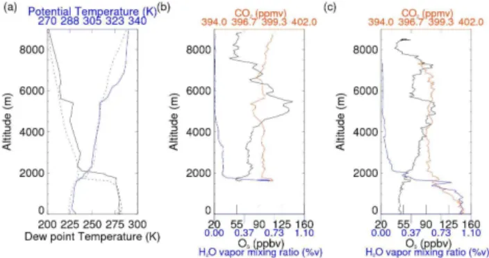
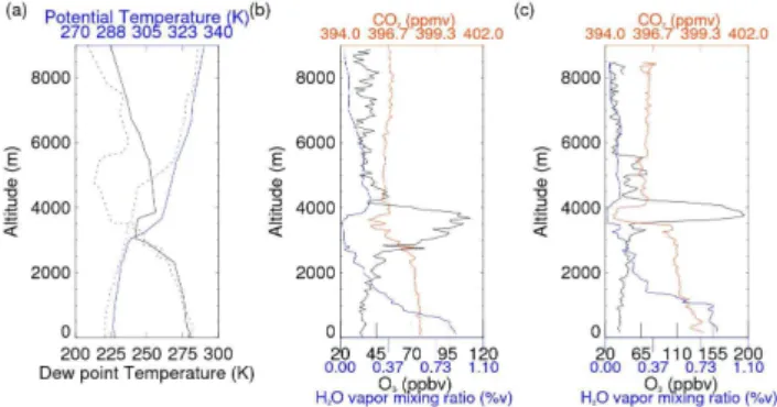
Figure 3 shows in situ measurements of potential temper-ature and dew point (Fig. 3a) and O3, CO2 and water
va-por (Fig. 3b, c). Potential temperature and dew point are taken from the most proximal radiosonde launches (Oakland (OAK)) and clearly identify a stable layer at 1.7 km, which existed before (dotted lines) and persisted after (solid lines) the time of the aircraft measurements. A pronounced dry, stable layer is present at 5.8 km in the radiosonde sounding taken∼5 h after aircraft measurements, identifying the ver-tical extent of the intrusion, associated with the cutoff low. This was not evident in the preceding radiosonde sounding as at that time the center of the cutoff low was still located to the west of OAK.
The O3, CO2and water vapor mixing ratios observed
dur-ing each profile are shown in Fig. 3b (offshore) and Fig. 3c (SJV). CO2 is a non-conventional tracer of stratospheric
air and provides an interesting comparison between strato-spheric and tropostrato-spheric air masses. A clear increase in O3is
observed between 4 and 7 km, a decrease in CO2between 4.5
and 5.5 km and reduced water vapor mixing ratios (< 0.015 percent by volume (%v)) at altitudes greater than 4 km in the offshore profile. Similar features are seen in the SJV pro-file, with an increase in O3 from > 2 km to 5.5 km and at
7 km, and a reduction in CO2and H2O mixing ratios at
al-titudes greater than 2 km, indicating the top of the boundary layer. The perturbations are more pronounced in the offshore profile, compared to the SJV profile where the O3lamina is
more vertically spread and as such has a slightly lower over-all maximum O3mixing ratio. However, the O3 maximum
and CO2and water vapor minima in both profiles are located
near 5 km.
CO2can be viewed as a more inert tracer than O3, since
it has no known sinks in the lower stratosphere (Aoki et al., 2003). The seasonal cycle of tropospheric CO2 has a large
amplitude characterized by a maximum in spring (April/May in the Northern Hemisphere) and minimum in summer (July) (Nakazawa et al., 1991; Boering et al., 1996; Hoor et al., 2004; Gurk et al., 2008; Sawa et al., 2008). In the lower stratosphere CO2has a less pronounced seasonal cycle with
low concentrations in winter–spring and higher concentra-tions in summer. From the seasonal cycle information pre-sented by Gurk et al. (2008) and Sawa et al. (2008), we ex-pect stratospheric CO2mixing ratios during the time of this
study (May–early June) to be less than tropospheric CO2
Fig. 2.5 km O3(ppbv) and wind vector (black, upper left) and PV (PVU) and wind vector (black, upper right) maps with O3(ppbv, lower
left) and PV (PVU, lower right) cross sections at 122◦W on 14 May 2012 at 18:00 UTC from the RAQMS analyses. The aircraft flight track
is shown in black. Oakland, located on the San Francisco East Bay, is shown as a red star. Note the cutoff low associated with relatively strong PV (bottom right) and high O3(bottom left) extending from the lower stratosphere into the mid-troposphere. The flight track and
observations were taken in a region were PV is < 2 PVU (bottom right), indicating STT occurrence (i.e., stratospheric air was sampled after crossing the tropopause). Black contours represent wind speed in m s−1.
Fig. 3. (a)Potential temperature (blue) and dew point (black) sound-ings at Oakland, CA, on 14 May 2012 at 12:00 UTC (dotted lines) and 15 May 2012 at 00:00 UTC (solid lines). Oakland is∼140 km from the San Joaquin Valley (inland) site and∼100 km from the offshore site. Mixing ratios of O3 (black), CO2 (red) and H2O (blue) observed(b) offshore, and(c)over the San Joaquin Valley during vertical profiles on 14 May 2012.
2012. As such, at this time of year in the Northern Hemi-sphere, CO2measurements collocated with O3and water
va-por can be used as tracers of STT. The use of additional trac-ers, such as CO2, further confirms the observed O3lamina to
be stratospheric in nature as opposed to aged and lofted Asian pollution, where CO2mixing ratios would be expected to be
representative of tropospheric values.
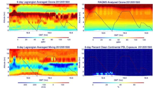
Figure 4 shows results of the RAQMS RDF curtain cal-culations for this flight along with the analyzed O3 curtain
(as described in Sect. 2.1). The RAQMS RDF O3shows a
much sharper vertical gradient in the upper troposphere than the analyzed O3 with RDF O3 in excess of 120 ppbv
be-low and 60 ppbv above 8 km. The sharp vertical gradients in the RDF calculation arise due to vertical shear, which leads to different horizontal sampling along the back trajec-tories and very different Lagrangian mean air-mass histrajec-tories at different altitudes. To determine which parts of the flight curtain may have been exposed to air within the continen-tal PBL, we track the amount of time each back trajectory spent within the continental PBL or is linked to the conti-nental PBL via convective mixing and then use 7-day (7–14 May 2013) averaged total column carbon monoxide (CO) from the Atmospheric Infrared Sounder (AIRS) (Aumann and Miller, 1995) to distinguish between exposure to clean and polluted continental PBL air. An AIRS total column CO threshold of 2.5×10⁸molecules cm−2was used
Fig. 4.RAQMS RDF O3(ppbv, upper left), analyzed O3 (ppbv, upper right), RDF mixing efficiency (m s−1, lower left), and % clean
continental PBL exposure (%, lower right) for AJAX flight on 14 May 2012.
exposure. By monitoring the amount of time that the back trajectories spent within either clean or polluted continental PBL, we can see that the air in the vicinity of the cutoff low was not within a clean continental PBL during the previous 6 days. The RAQMS RDF calculations predict no exposure to polluted continental PBL air along the aircraft flight track (not shown), which is consistent with the observed CO2.
The RDF mixing curtain provides a measure of the effi-ciency of large-scale mixing along the back trajectories and is determined from the Lagrangian averaged rate of stretch-ing of air parcels (Haynes and McIntyre, 1990; Fairlie et al., 2007). Regions of large positive RDF mixing (warm col-ors) are associated with strong shear flow where neighbor-ing air parcels can mix efficiently. Regions of large nega-tive RDF mixing (cool colors) are associated with rotational flow, where air parcels tend to remain more isolated. After 18:40 UTC (18.7 UTC), and above 6 km, the 14 May 2012 STT is associated with efficient large-scale mixing along the southern flank of the cutoff low, which leads to stretching of the air parcels and generation of laminar ozone features. Prior to 18:40 UTC (18.7 UTC) and below 6 km, the RDF curtain is within the rotational flow associated with the cutoff low (see Fig. 2); RDF mixing is negative, indicating that the air parcels have remained relatively isolated, inhibiting mixing between free-tropospheric and stratospheric air parcels.
This cutoff low provides an opportunity to evaluate the ability of the RAQMS O3analysis and RAQMS RDF O3to
capture the observed structure of the O3 lamina and to
as-sess the influence of numerical diffusion on predicted trans-port of stratospheric air into the troposphere. Figure 5 shows comparisons between the in situ O3measurements, RAQMS
O3analyses, and RAQMS RDF O3along the aircraft flight
track. The first encounter with the O3 lamina occurs prior
to 18:30 UTC (18.5 UTC) during the descending portion of the onshore (SJV) profile. During this flight leg both the RAQMS-analyzed and RDF O3 overestimate the observed
O3 mixing ratio, but the RDF O3 captures the sharp
verti-cal variations much better than the analyzed O3. Between
18:30 UTC and 18:48 UTC (18.5–18.8 UTC) the aircraft de-scends below 6 km and then begins to ascend again. Dur-ing this time period, when the aircraft is samplDur-ing within the cutoff low and the air is isolated from large-scale mix-ing, both the RAQMS RDF and analyzed O3are in relatively
good agreement with the in situ O3. Between 18:48 UTC and
19:12 UTC (18.8–19.2 UTC) the aircraft completes the as-cending portion of the onshore profile, reaches maximum al-titude, and conducts the descending portion of the offshore profile. During these legs the aircraft penetrates through the O3lamina twice, with in situ O3 ranging from 120 ppbv to
140 ppbv within the O3lamina and 60 ppbv above. The RDF
O3 does a very good job in capturing this variation while
the analyzed O3 shows a much broader O3 peak. The
nar-row O3 lamina captured by the RDF O3 analysis is poorly
resolved because of the relatively coarse horizontal and ver-tical resolution of RAQMS. As the scale of the O3 lamina
approaches the RAQMS grid dimensions, numerical diffu-sion becomes very large and the narrow feature is lost. After 19:12 UTC (19.2 UTC) the aircraft is again below 6 km and within the cutoff low where rotational flow dominates, and both the RDF and analyzed O3are in good agreement with
the in situ measurements.
The RAQMS back trajectories can be used to examine the history of the high (> 120 ppbv) RDF O3predicted within the
O3lamina. Figure 6 shows the back trajectory history and
Fig. 5.Time series of in situ (black), RAQMS reverse domain filled (RDF) (solid red), and RAQMS-analyzed (dashed red) O3(ppbv)
for AJAX flight on 14 May 2012. The in situ O3 data
acquisi-tion starts during the transit to the San Joaquin Valley (SJV) site. The first vertical profile is over the SJV and second vertical profile over the offshore location. The RDF approach provides much better agreement with the in situ observations.
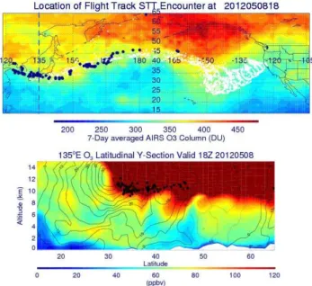
6 days prior to being sampled by the aircraft. The underlying map on the top of Fig. 6 shows 7-day averaged total column O3 from AIRS during the period from 7 to 14 May 2012.
The back trajectories show a significant amount of dispersion over the previous 6 days, with meridional spread in the back trajectories within the first 2–3 days and longitudinal spread 3–6 days prior to sampling by the aircraft. The majority of the high RDF O3values along the aircraft curtain were located to
the south of a region of high mean column O3off the coast of
Asia 6 days prior to sampling. At this time, the location of the air within the O3lamina that was sampled by the aircraft is an
elongated region extending north eastward from South Korea over southern Japan to about 45◦
N at the International Date Line. The bottom of Fig. 6 shows the RAQMS-analyzed O3
and zonal wind 135◦
E cross section at 18:00 UTC on 8 May 2012. The cross section shows that the air within the sampled O3lamina was located between 10 and 12 km on the
north-ern flank of a strong (> 60 m s−1) westerly jet at this time.
There are strong meridional gradients in O3 across the jet
axis, with high stratospheric O3on the poleward and lower
O3on the equatorward side of the jet. Analysis of the back
trajectories from the observed O3lamina at 18:00 UTC on 8
May 2012 shows that mean O3mixing ratio at the location
at 18:00 UTC on 8 May 2012 is 163 ppbv with a standard deviation of 50 ppbv. Efficient large-scale mixing of this ini-tial distribution with lower mixing ratio O3within the
tropo-sphere as well as numerical diffusion results in reductions in the mean and standard deviation in the analyzed O3lamina
to 97 ppbv and 7.5 ppbv, respectively, when it is sampled by the aircraft on 14 May 2012.
Fig. 6.Map of 7-day averaged (7–14 May 2012) AIRS total col-umn O3(DU, top) with the STT back trajectory history (white) and
locations of the high (> 120 ppbv) RDF O3mixing ratios (blue).
RAQMS 135◦E O3(ppbv) and zonal wind (black contours, m s−1)
cross section (bottom) with locations of the high (> 120 ppbv) RDF O3mixing ratios (blue dots) at 18:00 UTC on 8 May 2012 for anal-ysis of AJAX flight on 14 May 2012.
3.2 A post-trough, building ridge event: 5 June 2012
A deep, late-season extratropical cyclone affected California on 5 June 2012 and injected stratospheric air into the tropo-sphere, by means of a tropopause fold. The tropopause fold observed on 5 June 2012 was more pronounced, when com-paring maximum O3mixing ratios in each O3lamina, than
the event on 14 May 2012. Anomalously high O3 mixing
ratios were observed between 3 and 4 km, creating a steep O3 gradient between O3 within the tropopause fold (up to
120 ppbv offshore and 200 ppbv over SJV) and O3 in
sur-rounding air masses (40 and 50 ppbv offshore and over SJV respectively).
Figure 7 shows 4 km maps and 120◦
W cross sections of RAQMS O3and PV at 18:00 UTC on 5 June 2012. An
ex-tensive region of enhanced O3and PV over central California
at 4 km is being advected in from the northwest behind the trough. The RAQMS-analyzed O3 is greater than 80 ppbv,
and PV is in excess of 1.5 PVU indicating that stratospheric air (PV > 2 PVU) has crossed the tropopause. This enhanced O3 and PV extends down into the troposphere along the
northern flank of a relatively strong (45 m s−1) jet at 120◦
W. The aircraft flight path intersects the high O3 and PV
dur-ing the SJV profile and appears to be just to the south of the enhancement at 4 km during the offshore profile.
Fig. 7.4 km O3(ppbv) and wind vectors (black, upper left) and PV (PVU) and wind vectors (black, upper right) maps with O3 (ppbv,
lower left) and PV (PVU, lower right) cross sections at 120◦W on 5 June 2012 at 18:00 UTC from the RAQMS analyses. The aircraft flight
track is shown in black, Oakland, located on the San Francisco East Bay, is shown as a red star. Note the tropopause fold indicated by the tongue of relatively strong PV and high O3extending from the lower stratosphere into the mid-troposphere. The flight track and observations were taken in a region were PV is < 2 PVU (bottom right), indicating STT occurrence (i.e., stratospheric air was sampled after crossing the tropopause).
2012, 12:00 UTC, radiosonde sounding (dotted lines) and at 3 km in the 6 June 2012, 00:00 UTC, radiosonde sounding (solid lines). O3, CO2 and water vapor mixing ratios
ob-served during each profile are shown in Fig. 8b (offshore) and Fig. 8c (SJV). O3increases between 2.8–4 km offshore and
3.5–4.3 km over the SJV; an O3maximum in both instances
is observed at 3.7 km. The O3increase is more pronounced
in the SJV profile, compared to the offshore location. Also, in both profiles there are decreases in CO2and water vapor
mixing ratios at the same altitudes as the O3increases,
cor-roborating the assignment of stratospheric origin.
Figure 9 shows results of the RAQMS RDF curtain cal-culations for this flight along with the analyzed O3curtain.
The RDF and analyzed O3both show O3enhancements near
4 km during the first half of the flight (SJV profile), although the RDF O3shows sharper gradients and higher (> 100 ppbv)
mixing ratios than the analyzed O3. Neither RDF nor
ana-lyzed O3 shows significant enhancements during the latter
half of the flight (offshore profile) with peak O3mixing ratios
generally less than 70 ppbv at 3–4 km. The RDF mixing cur-tain shows that the lower half of the tropopause fold is associ-ated with negative mixing efficiencies, indicating that this air has remained relatively isolated during the previous 6 days.
Fig. 8. (a)Potential temperature (blue) and dew point (black) sound-ings at Oakland, CA, on 5 June 2012 at 12:00 UTC (dotted lines) and 6 June 2012 at 00:00 UTC (solid lines). Mixing ratios of O3
(black), CO2(red) and H2O (blue) observed(b)offshore, and(c)
over the San Joaquin Valley during descending, vertical profiles on 5 June 2012. Note the change of the O3horizontal scale between panels.
no exposure to polluted continental boundary layer air along the aircraft flight track (not shown).
Figure 10 shows comparisons between the in situ O3
measurements, RAQMS O3 analyses, and RAQMS RDF
O3 along the aircraft flight track. The aircraft samples the
tropopause fold three times prior to 19:00 UTC. During this period the RDF O3shows narrower features and somewhat
higher mixing ratios than the analyzed O3, but neither is able
to capture the amplitude of the observed O3peak, which is
greater than 150 ppbv during each of the three encounters and reaches 190 ppbv at 18:42 UTC (18.7 UTC) during the SJV profile. The aircraft is above the tropopause fold, between the first and second tropopause fold encounters, and the RDF O3captures the sharp vertical gradients and shows generally
better agreement with the in situ measurements. The aircraft is below the tropopause fold between the second and third tropopause fold encounters, and both RDF and analyzed O3
are in good agreement with the in situ measurements. The aircraft encounters the tropopause fold once at 19:30 UTC (19.5 UTC) during the offshore profile with both RDF and analyzed O3showing significant underestimates in O3.
Be-tween 19:36 and 19:48 UTC (19.6–19.8 UTC), the aircraft samples marine boundary layer where both the RDF and an-alyzed O3are in good agreement with the in situ
measure-ments. The tropopause fold is sampled for the fifth time be-tween 19:54 and 20:00 UTC (19.9–20.0 UTC), and both RDF and analyzed O3capture the observed vertical gradient, but
miss the high O3within the tropopause fold by up to 50 ppbv.
The RAQMS back trajectories are used to examine the history of the relatively high (> 80 ppbv) RDF O3
pre-dicted within the onshore tropopause fold feature. Figure 11 shows the back trajectory history and location of the high (> 80 ppbv) RDF O3mixing ratios beginning at 18:00 UTC
on 30 May 2012, 6 days prior to being sampled by the air-craft. The underlying map on the top of Fig. 11 shows 7-day averaged total column O3from AIRS during the period
from 29 May to 5 June 2012. During the first day prior to being sampled by the aircraft, the tropopause fold back tra-jectories remain very compact and move northwestward into a region south of Alaska with high AIRS average total col-umn O3. Three days prior to being sampled by the aircraft,
some of the tropopause fold back trajectories are dispersed further westward into the region of high AIRS average to-tal column O3over Japan and Siberia. However, the
major-ity of the tropopause fold back trajectories remain south of Alaska and circulate within a large, stationary low-pressure system near 150◦W. The bottom plot of Fig. 11 shows the
RAQMS-analyzed O3and zonal wind 150◦W cross section
at 18:00 UTC on 30 May 2012. The tropopause fold back tra-jectories were located within the core of the stationary low-pressure system in a region of moderately high O3and low
wind speeds between 6 and 8 km at this time. Analysis of the tropopause fold back trajectories at 18:00 UTC on 30 May 2012 shows that mean O3 mixing ratios at their location is
102 ppbv with a standard deviation of 14 ppbv, both of which
are significantly lower than found within the histories of the 14 May 2012 tropopause fold encounter. The low initial vari-ance of the 5 June 2012 tropopause fold back trajectories, combined with the fact that this tropopause fold encounter was associated with relatively isolated air and weak large-scale mixing, accounts for the smaller differences between the RDF and analyzed O3for this flight and indicates that
processes other than large-scale shear lead to the fine fila-ment structure observed on this flight. It is possible that dif-ferential transport by inertia gravity waves could have con-tributed to the formation of the thin filament of high O3,
given the close proximity of the flight to a strong jet core (see Fig. 7). For example, previous studies have reported sig-natures of small-scale vertical structures induced by inertia gravity waves in temperature, wind and ozone profiles (e.g., Danielsen et al., 1991; Pierce and Fairlie, 1993; Chane-Ming et al., 2003; Plougonven et al., 2003).
3.3 Stratosphere-to-troposphere implications
Due to changes in terrain and vertical transport, it is difficult to compare O3directly from two or more vertical profiles at
a particular altitude alone. Thus, to assess the contribution of the two STT events on the total mass of O3 within the
ob-served vertical profiles, the total measured O3was calculated
in Dobson units (DU) based upon the summation of the mea-sured O3 within a particular layer of the atmosphere (here,
measurements below ∼9 km (365 mbar) are used). To ac-count for terrain differences, the total O3in DU was
normal-ized by dividing by the thickness (mbar) of the atmosphere over which O3 measurements were taken (DU/100 mbar),
following the method of Cooper et al. (2011). The STT event on 14 May 2012 had a greater total O3DU/100 mbar value
compared to the 5 June 2012 event, even though the 14 May 2012 STT event had a reduced maximum O3 mixing ratio
compared to 5 June 2012. This is because the stratospheric intrusion on 14 May 2012 was more vertically extensive, and O3enhancements were measured over a wider altitude range
compared to the fine filament structure observed during the 5 June 2012 STT, which resulted in a larger overall enhance-ment of total O3within the 0–9 km layer.
For 14 May 2012, total O3 within the 0–9 km layer in
DU/100 mbar was 6.5 DU/100 mbar in the offshore profile and 6.9 DU/100 mbar above the SJV, compared to 4.2 and 3.8 DU/100 mbar in the offshore and SJV profiles respec-tively on 5 June 2012. For comparison, these values are within the range observed during the IONS-2010 campaign in May–June 2010 reported by Cooper et al. (2011), where typical values were within the range of 2–7 DU/100 mbar.
Given the importance of upper tropospheric O3in terms
Fig. 9.RAQMS RDF O3(ppbv, upper left), analyzed O3 (ppbv, upper right), RDF mixing efficiency (m s−1, lower left), and % clean
continental PBL exposure (%, lower right) for AJAX flight on 5 June 2012.
Fig. 10.Time series of in situ (black), RAQMS reverse domain filled (RDF) (solid red), and RAQMS-analyzed (dashed red) O3(ppbv) for AJAX flight on 5 June 2012. The first vertical profile is over the San Joaquin Valley and second vertical profile over the offshore location.
vertical resolution, to understand the frequency, magnitude and controlling processes of STT better.
The US EPA can currently exclude from the NAAQS O3
target any surface O3monitoring data identified as being
in-fluenced by an extreme stratospheric intrusion, since the nat-urally occurring “exceptional events” are uncontrollable by state agencies. However, identification of STT contributing to surface O3sites remains challenging for several reasons,
including a lack of vertical O3 measurements, which
iden-tify the extent of the intrusion, and the limited effectiveness of models in forecasting the impacts of STT in part due to the complex topography of the western United States and re-sulting mesoscale dynamics (e.g., mountain lee waves and low-level jets). Furthermore, stratospheric intrusions can re-main aloft or contribute to the overall background by
grad-Fig. 11.Map of 7-day averaged (30 May–5 June 2012) AIRS total column O3(DU, top) with the STT back trajectory history (white)
and origin (blue) and RAQMS 150◦W O
3(ppbv) and zonal wind
(m s−1) cross section (bottom) with origin of STT encounter (blue
dots) at 18:00 UTC on 30 May 2012 for analysis of AJAX flight on 5 June 2012.
ual mixing with the boundary layer making a distinct O3
enhancement difficult to distinguish, and the effects of a stratospheric intrusion may result in an increase of O3 at
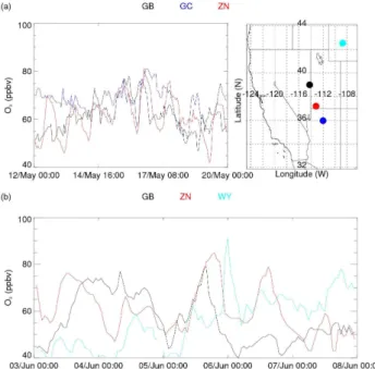
Fig. 12.O3time series from surface monitoring sites: Great Basin
National Park, Nevada (GB, black); Grand Canyon National Park, Arizona (GC, blue); Zion National Park, Utah (ZN, red); and South Pass, Wyoming (WY, cyan), during 12–19 May 2012(a)and 3–7 June 2012(b).
be potentially entrained into the boundary layer and impact surface sites, particularly when considering the mountainous terrain of the western United States and convection during springtime, both of which intensify vertical mixing.
Maps of the US EPA air quality index from 5 to 6 June 2012 showed moderate to high O3 over parts of
Califor-nia, Nevada, Utah and Wyoming, with exceedances of the NAAQS O3standard in southwestern Utah, eastern Nevada
and Wyoming (www.airnow.gov). Potential vorticity and O3
from the 18:00 UTC RAQMS analysis for 5 June 2012 also show how the tropopause fold descends to low altitudes (< 4 km) over California, Nevada, Utah and east to 111◦
W. To investigate the possibility of STT contributing to surface-level O3 further, one-hour O3 mixing ratios were obtained
from rural sites in Grand Canyon National Park, Arizona (GC); Great Basin National Park, Nevada (GB); South Pass, Wyoming (WY); and Zion National Park, Utah (ZN).
Assessment of the impacts of STT on surface sites for the 14 May 2012 STT event proved difficult. Air quality maps from 14 May 2012 show enhanced O3over southern
Califor-nia, southern and eastern Nevada, Arizona and Utah. Time-series plots of the one-hour surface O3from GB, ZN and GC
show a general increase in the diurnal cycle of surface O3
during 15–16 May 2012 compared to the days before and af-ter. However, there is no distinct enhancement outside of the daytime periods, making the potential contribution from STT difficult to assess (see Fig. 12a).
Enhancements of surface O3are observed during 5–6 June
2012 (see Fig. 12b). Maximum surface O3 enhancements
at GB and ZN occur on 5 June 2012 reaching 79 ppbv at 16:00 (local time) at GB and 85 ppbv at 19:00 (local time) at ZN. However, the occurrences during daytime hours com-plicate identification of STT influence at these sites. At the WY site, a distinct increase in O3is observed with a
max-imum of 91 ppbv measured at 00:00 (local time) on 6 June 2012. This is clearly not a result of photochemical process-ing and as such is most likely evidence of the impact of STT at surface sites. An assessment of the meteorological data supports this conclusion; the upper level disturbance, which resulted in the tropopause fold observed in-flight on 5 June 2012, had moved east and was lying directly upstream of the South Pass surface O3site in western Wyoming.
Corre-sponding PV time–height cross-section analysis adds further support, with a descending≥1 PVU isoline over Wyoming (data not shown) through 5–6 June 2012. Forward trajecto-ries from Hybrid Single Particle Trajectory Integrated Trajec-tory model (HYSPLIT-WEB (internet-based)) also confirm the eastward movement of the system and the descending tra-jectory from 5 km at 18:00 UTC on the 5 June 2012 over the offshore and inland vertical profile sites with some ensem-ble trajectories intersecting with ground level over Wyoming (Draxer and Rolph, 2013).
4 Conclusions
The difference in the trace gas composition of the strato-sphere compared to the tropostrato-sphere permits the identification of air masses of stratospheric origin found within the free troposphere occurring during STT. In this paper two STT case studies, sampled over California, were presented: one on 14 May 2012 associated with a cutoff low and one on 5 June 2012 occurring within a tropopause fold during a post-trough, building ridge event.
In each case, a region of enhanced O3, an O3lamina, was
observed and at altitudes as low as 3 km above sea level. During both events the stratospheric air was characterized by high O3and low water vapor and CO2mixing ratios. The
ob-servation of decreased CO2within the stratospheric air mass
is consistent with the varying seasonal cycles of CO2in the
troposphere and stratosphere and provides evidence and sup-port for the use of in situ CO2measurements as an additional
method for detecting STT events.
RAQMS O3analysis and RDF diagnostics provide a
large-scale context for the interpretation of the airborne measure-ments. RDF results show that the two STT events had very different air mass histories. The 14 May 2012 O3lamina was
associated with a tropopause fold developing from a cutoff low-pressure system that moved into central California from the southwest and experienced efficient large-scale mixing during the previous 6 days. As a result, the O3 lamina was
longitudinal range with considerable initial variability in O3
mixing ratios. In contrast, the back trajectories from the 5 June 2012 tropopause fold showed its history from within the core of a large, stationary low-pressure system over the Gulf of Alaska, which remained relatively isolated with very little large-scale mixing during the previous 6 days. Compar-isons between the in situ O3and RAQMS RDF and analyzed
O3along the flight track show that the RDF O3was able to
do a very good job in capturing the high ozone within the 14 May 2012 O3lamina, while the analyzed O3was not able
to maintain the strong vertical gradients that were observed. This was attributed to increasing numerical diffusion as the scale of the STT event approached the model grid scale. Nei-ther the RDF nor analyzed O3was able to capture the high
O3observed during the 5 June 2012 tropopause fold.
The impact of the two STT events on the 0–9 km O3
bud-get has been assessed by comparing the total,measured 0– 9 km O3(DU) from each analysis day. The STT event on 14
May 2012, although displaying a smaller O3maximum
mix-ing ratio, had a greater total O3DU value in the 0–9 km layer
than the 5 June 2012 STT event. The fine filament structure of the O3lamina on 5 June 2012 would make it difficult to
detect this STT event from O3column measurements.
How-ever, narrow filaments could likely be detected by other re-mote sensing techniques such as O3 lidar. Given clear sky
conditions, O3 lidar measurements provide frequent
mea-surements of O3profiles over a specific site (if surface-based)
providing good temporal coverage but limited spatial cov-erage. O3lidar potentially provides complementary data to
aircraft measurements, which provide good spatial and verti-cal coverage but limited temporal coverage. This work high-lights the importance of O3vertical profile measurements in
the detection of STT, which in some cases, depending on lo-cation and the fine-scale structure of O3laminae, may be the
only way to detect and analyze different occurrences of STT accurately.
Investigations were conducted to assess the potential im-pacts of these STT events on rural surface O3 monitoring
sites. Evidence supporting the influence of stratospheric air masses on monitoring sites was detected, with a particu-lar O3episode exceeding NAAQS O3standard measured at
South Pass, Wyoming, likely associated with the observed tropopause fold on 5 June 2012. More quantitative support for the influence of stratospheric air masses on surface O3
requires additional airborne measurements and multi-scale, nested modeling approaches. This study has shown that the RAQMS global O3analyses underestimate the high O3
mix-ing ratios observed in both STT events. As a result, higher resolution modeling studies using global-scale O3 analyses
for lateral boundary conditions likely underestimate the mag-nitude of the exceedances due to STT. Preliminary com-parisons between South Pass, Wyoming, surface O3
obser-vations and predictions from nested RAQMS/WRF-CHEM 8 km simulations of the June STT event confirm this.
Acknowledgements. The authors gratefully recognize the support
and partnership of H211 L. L. C., with particular thanks to K. Am-brose, R. Simone, B. Quiambao, J. Lee, J. McMahon, and R. Fisher. Funding was provided by the NASA Postdoctoral Program (J. T.), San Jose State University Research Foundation (E. Y.), and the Bay Area Environmental Research Institute (M. R.). Funding for instrumentation and aircraft integration is gratefully acknowledged from Ames Research Center Director’s funds. Helpful discussions with R. S. Hipskind, P. Hamill, L. Pfister and R. Chatfield are happily acknowledged. Technical contributions from Z. Young, E. Quigley, R. Walker, and A. Trias made this project possible. The views, opinions, and findings contained in this report are those of the author(s) and should not be construed as an official National Oceanic and Atmospheric Administration or US Government position, policy, or decision.
Edited by: H. Wernli
References
Aoki, S., Nakazawa, T., Machida, T., Sugawara, S., Morimoto, S., Hashida, G., Yamanouchi, T., Kawamura, K., and Honda, H.: Carbon dioxide variations in the stratosphere over Japan, Scandi-navia and Antarctica, Tellus B, 55, 178–186, doi:10.1034/j.1600-0889.2003.00059.x, 2003.
Aumann, H. H. and Miller, C.: Atmospheric Infrared Sounder (AIRS) on the Earth Observing System, SPIE, 2583, 32–343, doi:10.1117/12.228579, 1995.
Boering, K. A., Wofsy, S. C., Daube, B. S., Schneidner, H. R., Loewenstein, M., Podolski, J. R., and Conway, T. J.: Strato-spheric mean ages and transport rates from observations of carbon dioxide and nitrous oxide, Science, 22, 1340–1343, doi:10.1126/science.274.5291.1340, 1996.
Bonasoni, P., Evangelisti, F., Bonafe, U., Ravegnani, F., Calzolari, F., Stohl, A., Tositti, L., Tubertini, O., and Colombo, T.: Strato-spheric ozone intrusion episodes recorded at Mt. Cimone during the VOTALP project: case studies, Atmos. Environ., 34, 1355– 1365, 2000.
Bourqui, M. S. and Trépanier, P.-Y.: Descent of deep stratospheric intrusions during the IONS August 2006 campaign, J. Geophys. Res., 115, D18301, doi:10.1029/2009JD013183, 2010.
Bowman, K. P., Pan, L. L., Campos, T., and Gao, R.: Observa-tions of fine-scale transport structure in the upper troposphere from the High-performance Instrumented Airborne Platform for Environmental Research, J. Geophys. Res., 112, D18111, doi:10.1029/2007JD008685, 2007.
Chane-Ming, F., Guest, F., and Karloy, D. J.: Gravity waves ob-served in temperature, wind and ozone data over Macquarie Is-land, Aust. Meteorol. Mag., 52, 11–21, 2003.
Chung, Y. S. and Dann, T.: Observations of stratospheric ozone at the ground level in Regina, Canada., Atmos. Environ., 19, 157– 162, doi:10.1016/0004-6981(85)90147-7, 1985.
Cooper, O. R., Oltmans, S. J., Johnson, B. J., Brioude, J., Angevine, W., Trainer, M., Parrish, D. D., Ryerson, T. R., Pollack, I., Cullis, P. D., Ives, M. A., Tarasick, D. W., Al-Saadi, J., and Stajner, I.: Measurement of western U.S. baseline ozone from the surface to the tropopause and assessment of downwind impact regions, J. Geophys. Res., 116, D00V03, doi:10.1029/2011JD016095, 2011.
Danielsen, E. F.: Stratospheric-tropospheric exchange based on ra-dioactivity, ozone and potential vorticity, J. Atmos. Sci., 25, 502– 518, 1968.
Danielsen, E. F. and Mohnen, V. A.: Project duststorm report: ozone transport, in-situ measurements, and meteorological anal-ysis of tropopause folding, J. Geophys. Res., 82, 5867–5877, doi:10.1029/JC082i037p05867, 1977.
Danielsen, E. F., Hipskind, R. S., Starr, W. L., Vedder, J. F., Gaines, S. E., Klev, D., and Kelly, K. K.: Irreversible transport in the stratosphere by internal waves of short vertical wavelength, J. Geophys. Res., 96, 17433–17452, doi:10.1029/91JD01362, 1991.
Draxer, R. R. and Rolph, G. D.: HYSPLIT (HYbrid Single Particle Lagrangian Integrated Trajectory) Model access via NOAA ARL READY website http://www.arl.noaa.gov/HSPLIT.php (last ac-cess: 30 September 2013), NOAA Air Resources Laboratory, College Park, MD, 2013.
Ebel, A., Hass, H., Jakobs, H. J., Laube, M., Memmesheimer, M., Oberreuter, A., Geiss, H., and Kuo, Y.-H.: Simulation of ozone intrusion caused by a tropopause fold and cut-off low, Atmos. Environ., 25, 2131–2144, 1991.
Fairlie, T. D., Avery, M. A., Pierce, R. B., Al-Saadi, J., Dibb, J., and Sachse, G.: Impact of multiscale dynamical processes and mixing on the chemical composition of the upper tropo-sphere and lower stratotropo-sphere during the Intercontinental Chemi-cal Transport Experiment–North America, J. Geophys. Res., 112, D16S90, doi:10.1029/2006JD007923, 2007.
Fiore, A., Jacob, D. J. Liu, H., Yantosca, R. M., Fairlie, T. D., and Li, Q.: Variability in surface ozone background over the United States: Implications for air quality policy, J. Geophys. Res., 108, 4787, doi:10.1029/2003JD003855, 2003.
Gurk, Ch., Fischer, H., Hoor, P., Lawrence, M. G., Lelieveld, J., and Wernli, H.: Airborne in-situ measurements of vertical, seasonal and latitudinal distributions of carbon dioxide over Europe, At-mos. Chem. Phys., 8, 6395–6403, doi:10.5194/acp-8-6395-2008, 2008.
Haynes, P. H. and McIntyre, M. E.: On the conservation and im-permeability theorems for potential vorticity, J. Atmos. Sci., 47, 2021–2031, 1990.
Hocking, W. K., Carey-Smith, T., Tarasick, D. W., Argall, P. S., Strong, K., Rochon, Y., Zawadzki, I., and Taylor, P. A.: Detection of stratospheric ozone intrusions by windprofiler radars, Nature, 450, 281–284, 2007.
Hoor, P., Gurk, C., Brunner, D., Hegglin, M. I., Wernli, H., and Fischer, H.: Seasonality and extent of extratropical TST derived from in-situ CO measurements during SPURT, Atmos. Chem. Phys., 4, 1427–1442, doi:10.5194/acp-4-1427-2004, 2004. IPCC (Intergovernmental Panel on Climate Change, Climate
Change): The Physical Science Basis, Summary for Policymak-ers – Contribution of Working Group I to the Fourth Assessment Report of the Intergovernmental Panel on Climate Change, Cam-bridge University Press, New York, 2007.
Kleist, D. T., Parrish, D. F., Derber, J. C., Treadon, R., Wu, W.-S., and Lord, S.: Introduction of the GSI into the NCEP Global Data Assimilation System, Weather Forecast., 24, 1691–1705, 2009. Lamarque, J.-F. and Hess, P. G.: Cross-tropopause mass exchange
and potential vorticity budget in a simulated tropopause folding, J. Atmos. Sci., 51, 2246–2269, 1994.
Langford, A. O., Aikin, K. C., Eubank, C. S., and Williams, E. J.: Stratospheric contribution to high surface ozone in Col-orado during springtime, Geophys. Res. Lett., 36, L12801, doi:10.1029/2009GL038367, 2009.
Langford, A. O., Brioude, J., Cooper, O. R., Senff, C. J., Alvarez II, R. J., Hardesty, R. M., Johnson, B. J., and Oltmans, S. J.: Stratospheric influence on surface ozone in the Los Angeles area during late spring and early summer of 2010, J. Geophys. Res., 117, D00V06, doi:10.1029/2011JD016766, 2012.
Lefohn, A. S., Wernli, H., Shadwick, D., Limbach, S., Olt-mans, S. J., and Shapiro, M.: The importance of stratospheric-tropospheric transport in affecting surface O3 mixing ratios in
the western United States, Atmos. Environ., 45, 4845–4857, doi:10.1016/j.atmosenv.2011.06.014, 2011.
Lefohn, A. S., Wernli, H., Shadwick, D., Oltmans, S., and Shapiro, M.: Quantifying the importance of stratosphere-troposphere transport on surface ozone concentrations at high- and low- el-evation monitoring sites in the United States, Atmos. Environ., 62, 646–656, doi:10.1016/j.atmosenv.2012.09.004, 2012. Levelt, P. F., van den Oord, G. H. J., Dobber, M. R., Mälkki, A.,
Visser, H., de Vries, J., Stammes, P., Lundell, J. O. V., and Saari, H.: The Ozone Monitoring Instrument, IEEE T. Geosci. Remote, 44, 1093–1101, doi:10.1109/TGRS.2006.872333, 2006. Lin, M., Fiore, A. M., Cooper, O. R., Horowitz, L. W., Langford, A.
O., Levy II, H., Johnson, B. J., Naik, V., Oltmans, S. J., and Senff, C. J.: Springtime high surface ozone events over the western United States: Quantifying the role of stratospheric intrusions, J. Geophys. Res., 117, D00V22, doi:10.1029/2012JD018151, 2012.
Nakazawa, T., Miyashita, K., Aoki, S., and Tanaka, M.: Temporal and spatial variations of upper troposphere and lower stratospheric carbon dioxide, Tellus B, 43, 106–117, doi:10.1034/j.1600-0889.1991.t01-1-00005.x, 1991.
Pierce, R. B. and Fairlie, T. D. A.: Chaotic advection in the strato-sphere: Implications for the dispersal of chemically perturbed air from the polar vortex, J. Geophys. Res., 98, 18589–18595, 1993. Pierce, R. B., Grose, W. L., Russell III, J. M., and Tuck, A. F.: Evolution of southern hemisphere spring air masses observed by HALOE, Geophys. Res. Lett., 21, 213–216, doi:10.1029/93GL02997, 1994.
Pierce, R. B., Schaack, T. K., Al-Saadi, J., Fairlie, T. D., Kittaka, C., Lingenfelser, G., Natarajan, M., Olson, J., Soja, A., Zapo-tocny, T. H., Lenzen, A., Stobie, J., Johnson, D. R., Avery, M., Sachse, G., Thompson, A., Cohen, R., Dibb, J., Crawford, J., Rault, D., Martin, R., Szykman, J., and Fishman, J.: Chemi-cal data assimilation estimates of continental US ozone and ni-trogen budgets during the Intercontinental Chemical Transport Experiment – North America, J. Geophys. Res., 112, D12S21, doi:10.1029/2006JD007722, 2007.
the TexAQS field mission, J. Geophys. Res., 114, D00F09, doi:10.1029/2008JD011337, 2009.
Plougonven, R., Teitelbaum, H., and Zeitlin, V.: Inertia gavity wave generation by the tropospheric midlatitude jet as given by the Fronts and Atlantic Storn-Track Experiment radio soundings, J. Geophys. Res., 108, 4686, doi:10.1029/2003JD003535, 2003. Sawa, Y., Machida, T., and Matsueda, H.: Seasonal variations of
CO2 near the tropopause observed by commercial aircraft, J. Geophys. Res. 113, D23301, doi:10.1029/2008JD010568, 2008. Schaack, T. K., Zapotocny, T. H., Lenzen, A. J., and Johnson, D. R.: Global Climate Simulation with the University of Wiscon-sin Global Hybrid Isentropic Coordinate Model, J. Climate, 17, 2998–2016, 2004.
Skerlak, B., Sprenger, M., and Wernli, H.: A global climatol-ogy of stratosphere-troposphere exchange using the ERA-interim dataset from 1979 to 2011, Atmos. Chem. Phys. Discuss., 13, 11537–11595, doi:10.5194/acpd-13-11537-2013, 2013. Søensen, J. H. and Nielson, N. W.: Intrusion of stratospheric ozone
to the free troposphere through tropopause folds – A case study, Phys. Chem. Earth Pt. B, 26, 801–806, 2001.
Sprenger, M. and Wernli, H.: A northern hemispheric climatology of cross-tropopause exchange for the ERA15 time period (1979– 1993), J. Geophys. Res., 108, 8521, doi:10.1029/2002JD002636, 2003.
Sprenger, M., Croci Maspoli, M., and Wernli, H.: Tropopause folds and cross-tropopause exchange: A global investiga-tion based upon ECMWF analyses for the time period March 2000 to Februray 2001, J. Geophys. Res., 108, 8513, doi:10.1029/2002JD002587, 2003.
Stohl, A., Spichtinger-Rakowsky, N., Bonasoni., P., Feldman, H., Memmesheimer, M., Scheel, H. E., Trickl, T., Hübener, S., Ringer, W., and Mandl, M.: The influence of stratospheric in-trusions on alpine ozone concentrations, Atmos. Environ., 34, 1323–1354, 2000.
Stohl, A., Bonasoni, P., Cristofanelli, P., Collins, W., Feichter, J., Frank, A., Forster, C., Gerasopoulos, E., Gäggeler, H., James, P., Kentarchos, T., Kromp-Kolb, H., Krüger, B., Land, C., Meloen, J., Papayannis, A., Priller, A., Seibert, P., Sprenger, M., Roelofs, G. J., Scheel, H. E., Schnabel, C., Siegmund, P., To-bler, L., Trickl, T., Wernli, H., Wirth, V., Zanis, P., and Zere-fos, C.: Stratosphere-troposphere exchange: A review, and what we have learned from STACCATO, J. Geophys. Res., 108, 8516, doi:10.1029/2002JD002490, 2003.
Sutton, R. T., Maclean, H., Swinbank, R., O’Neill, A., and Taylor, F. W.: High-resolution stratospheric tracer fields estimated from satellite observations using Lagrangian trajectory calculations, J. Atmos. Sci., 51, 2995–3005, 1994.
Thompson, A. M., Stone, J. B., Witte, J. C., Miller, S. K., Pierce, R. B., Chatfield, R. B., Oltmans, S. J., Cooper, O. R., Loucks, A. L., Taubman, B. F., Johnson, B. J., Joseph, E., Kucsera, T. L., Mer-rill, J. T., Morris, G. A., Hersey, S., Forbes, G., Newchurch, M. J., Schmidlin, F. J., Tarasick, D. W., Thouret, V., and Cammas, J.-P.: Intercontinental chemical transport experiment Nzonesonde Network Study (IONS) 2004: 1. Summertime upper tropo-sphere/lower stratosphere ozone over northeastern North Amer-ica, J. Geophys. Res., 112, D12S12, doi:10.1029/2006JD007441, 2007.
Trickl, T., Bärtsch-Ritter, N., Eisele, H., Furger, M., Mücke, R., Sprenger, M., and Stohl, A.: High-ozone layers in the middle and upper troposphere above Central Europe: potential import from the stratosphere along the subtropical jet stream, Atmos. Chem. Phys., 11, 9343–9366, doi:10.5194/acp-11-9343-2011, 2011. US Environmental Protection Agency, US EPA: Air quality
cri-teria for ozone and related photochemical oxidants, report EPA/600/R-05/004af, Office of Research and Development, Re-search Triangle Park, NC. February 2006, US Environmental Protection Agency, 2006.
US Environmental Protection Agency, US EPA: National Ambient Air Quality Standards for Ozone, Federal Register FRL-9102-1, 2938–3052, 2010.
Vaughan, G., Price, J. D., and Howells, A.: Transport into the tropo-sphere in a tropopause fold, Q. J. Roy. Meteor. Soc., 120, 1085– 1103, 1994.
Waters, J. W., Froidevaux, L., Harwood, R. S., Jarnot, R. F., Pick-ett, H. M., Read, W. G., Siegel, P. H., Cofield, R. E., Filipiak, M. J., Flower, D. A., Holden, J. R., Lau, G. K., Livesey, N. J., Manney, G. L., Pumphrey, H. C., Santee, M. L., Wu, D. L., Cuddy, D. T., Lay, R. R., Loo, M. S., Perun, V. S., Schwartz, M. J., Stek, P. C., Thurstans, R. P., Boyles, M. A., Chandra, K. M., Chavez, M. C., Chen, G.-S., Chudasama, B. V., Dodge, R., Fuller, R. A., Girard, M. A., Jiang, J. H., Jiang, Y., Knosp, B. W., LaBelle, R. C., Lam, J. C., Lee, K. A., Miller, D., Oswald, J. E., Patel, N. C., Pukala, D. M., Quintero, O., Scaff, D. M., Sny-der, W. V., Tope, M. C., Wagner, P. A., and Walch, M. J.: The Earth Observing System Microwave Limb Sounder (EOS MLS) on the Aura Satellite, IEEE T. Geosci. Remote, 44, 1075–1092, doi:10.1109/TGRS.2006.873771, 2006.
Worden, H. M., Bowman, K. W., Worden, J. R., Eldering, A., and Beer, R.: Satellite measurements of the clear-sky greenhouse ef-fect from tropospheric ozone, Nat. Geosci., 1, 305–308, 2008. World Meteorological Organisation, WMO: Atmospheric ozone
1985: Global ozone research and monitoring report, WMO Rep. 16, Geneva, 1986.
Zanis, P., Trickl, T., Stohl, A., Wernli, H., Cooper, O., Zerefos, C., Gaeggeler, H., Schnabel, C., Tobler, L., Kubik, P. W., Priller, A., Scheel, H. E., Kanter, H. J., Cristofanelli, P., Forster, C., James, P., Gerasopoulos, E., Delcloo, A., Papayannis, A., and Claude, H.: Forecast, observation and modelling of a deep stratospheric intrusion event over Europe, Atmos. Chem. Phys., 3, 763–777, doi:10.5194/acp-3-763-2003, 2003.