Assessing variability and long-term trends in burned area by merging multiple satellite fire products

(1)

BGD

6, 11577–11622, 2009

Assessing burned area variability and

trends

L. Giglio et al.

Title Page

Abstract Introduction

Conclusions References

Tables Figures

◭ ◮

Back Close

Full Screen / Esc

Printer-friendly Version

Interactive Discussion

Biogeosciences Discuss., 6, 11577–11622, 2009 www.biogeosciences-discuss.net/6/11577/2009/ © Author(s) 2009. This work is distributed under the Creative Commons Attribution 3.0 License.

Biogeosciences Discussions

This discussion paper is/has been under review for the journal Biogeosciences (BG). Please refer to the corresponding final paper in BG if available.

Assessing variability and long-term

trends in burned area by merging multiple

satellite fire products

L. Giglio1,2, J. T. Randerson3, G. R. van der Werf4, P. S. Kasibhatla5,

G. J. Collatz1, D. C. Morton1, and R. S. DeFries6

1

NASA Goddard Space Flight Center, Greenbelt, Maryland, USA 2

Department of Geography, University of Maryland, College Park, Maryland, USA 3

Department of Earth System Science, University of California, Irvine, California, USA 4

Faculty of Earth and Life Sciences, VU University, Amsterdam, The Netherlands 5

Nicholas School of the Environmental and Earth Sciences, Duke University, Durham, North Carolina, USA

6

Department of Ecology, Evolution, and Environmental Biology, Columbia University, New York, USA

Received: 20 November 2009 – Accepted: 9 December 2009 – Published: 18 December 2009

Correspondence to: L. Giglio (louis [email protected])

(2)

BGD

6, 11577–11622, 2009

trends

L. Giglio et al.

Title Page

Tables Figures

◭ ◮

Back Close

Full Screen / Esc

Abstract

Long term, high quality estimates of burned area are needed for improving both prog-nostic and diagprog-nostic fire emissions models and for assessing feedbacks between fire and the climate system. We developed global, monthly burned area estimates aggre-gated to 0.5◦ spatial resolution for the time period July 1996 through mid-2009 using

5

four satellite data sets. From 2001–2009, our primary data source was 500-m burned area maps produced using Moderate Resolution Imaging Spectroradiometer (MODIS) surface reflectance imagery; more than 90% of the global area burned during this time period was mapped in this fashion. During times when the 500-m MODIS data were not available, we used a combination of local regression and regional regression trees

10

to develop relationships between burned area and Terra MODIS active fire data. Cross-calibration with fire observations from the Tropical Rainfall Measuring Mission (TRMM) Visible and Infrared Scanner (VIRS) and the Along-Track Scanning Radiometer (ATSR) allowed the data set to be extended prior to the MODIS era. With our data set we esti-mated the global annual area burned for the years 1997–2008 varied between 330 and

15

431 Mha, with the maximum occurring in 1998. We compared our data set to the recent GFED2, L3JRC, GLOBCARBON, and MODIS MCD45A1 global burned area products and found substantial differences in many regions. Lastly, we assessed the interan-nual variability and long-term trends in global burned area over the past 12 years. This burned area time series serves as the basis for the third version of the Global Fire

20

Emissions Database (GFED3) estimates of trace gas and aerosol emissions.

1 Introduction

As Earth-system modeling e_fforts increasingly recognize and include fire as an im-portant process in the terrestrial carbon cycle, there remains a strong need for long term, spatially- and temporally-explicit global burned area data sets. Among other

pur-25

(3)

emis-BGD

6, 11577–11622, 2009

trends

L. Giglio et al.

Title Page

Tables Figures

◭ ◮

Back Close

Full Screen / Esc

sions, discriminating natural versus anthropogenic contributions to global change, and identifying feedbacks between fire and climate change (Langmann et al., 2009). In response to this need, a growing number of multi-year, satellite-based global burned area products have been made publicly available over the past several years. These include: 1) the 1-km L3JRC product (Tansey et al., 2008), currently spanning April

5

2000–March 2007, and produced from SPOT VEGETATION imagery with a modified version of the Tansey et al. (2004) Global Burnt Area (GBA) 2000 algorithm; 2) the 1-km GLOBCARBON burned area product, currently spanning April 1998–December 2007, derived from SPOT VEGETATION, Along-Track Scanning Radiometer (ATSR-2), and Advanced ATSR (AATSR) imagery using a combination of mapping algorithms

(Plum-10

mer et al., 2006); and 3) the Roy et al. (2008) 500-m Moderate Resolution Imaging Spectroradiometer (MODIS) burned area product (MCD45A1), generated from Terra and Aqua MODIS imagery and available from mid-2000 through the present. All three data sets map the spatial extent of burned vegetation (variously referred to asburned areas, burnt areas, burn scars, fire scars, and fire-affected areas) at daily temporal

15

resolution. At coarser spatial and temporal scales, the version 2 Global Fire Emissions Database (GFED2) provides monthly global burned area estimates at 1◦ spatial res-olution from January 1997–December 2008. In GFED2, burned area was estimated indirectly using monthly active fire observations from the MODIS, ATSR, and Tropi-cal Rainfall Measuring Mission (TRMM) Visible and Infrared Scanner (VIRS) sensors

20

(Giglio et al., 2006b; van der Werf et al., 2006).

Here we describe the next generation of the Global Fire Emissions Database burned area data set – GFED3 – which provides global, monthly burned area aggregated to 0.5◦ spatial resolution from mid-1996 through the present, and is specifically intended for use within large-scale (typically global) atmospheric and biogeochemical models.

25

(4)

BGD

6, 11577–11622, 2009

trends

L. Giglio et al.

Title Page

Tables Figures

◭ ◮

Back Close

Full Screen / Esc

set are spatially-explicit uncertainties that reflect the varying quality of the burned area estimates produced from each source and methodology. Following a summary of the input data in Sect. 2 and a description of our methods in Sect. 3, we use the GFED3 data set to assess the interannual variability and long-term trends in global burned area over the past 13 years in Sect. 4, and then compare it to the independent L3JRC,

5

GLOBCARBON, and Collection 5 MODIS MCD45A1 global burned area products in Sect. 5.

2 Data

2.1 Burned area data

Reference burned area maps were produced from the 500-m MODIS

atmospherically-10

corrected Level 2G surface reflectance product (Vermote and Justice, 2002), the MODIS Level 3 daily active fire products (Justice et al., 2002), and the MODIS Level 3 96-day land cover product (Friedl et al., 2002) using the Giglio et al. (2009) MODIS direct broadcast burned area mapping algorithm. The algorithm identifies the date of burn (to the nearest day) for each grid cell within individual MODIS Level 3 tiles (Wolfe

15

et al., 1998).

Selected calendar months were processed for most MODIS land tiles, yielding a to-tal of approximately 8300 “tile-months” of burned area maps between November 2000 and July 2009. This is nearly 19 times the quantity of training data used to produce the GFED2 burned area data set (Giglio et al., 2006b). The resulting maps were

aggre-20

gated to 0.5◦spatial resolution and monthly temporal resolution.

2.2 Active fire data

(5)

BGD

6, 11577–11622, 2009

trends

L. Giglio et al.

Title Page

Tables Figures

◭ ◮

Back Close

Full Screen / Esc

through mid-2009. We also used the Giglio et al. (2003) 0.5◦ gridded monthly VIRS fire product, from January 1998 through December 2008, and the ATSR World Fire Atlas (algorithm 2) from July 1996 through December 2007 (Arino and Rosaz, 1999). For compatibility the ATSR fire locations were gridded to produce monthly 0.5◦ ATSR fire counts.

5

3 Method

As an interim product based on a small quantity of 500-m burned area training data, the GFED2 burned area data set was composed solely of indirect burned area estimates derived from gridded active fire counts. In that approach, a series of regional regres-sion trees were used to relate monthly active-fire and ancillary land cover information

10

to monthly area burned at 1◦ spatial resolution (Giglio et al., 2006b). The enormous quantity of 500-m MODIS burned area training data we have produced since that earlier work, however, has allowed us to incorporate several major refinements into GFED3. First, the spatial resolution of the global grid was quadrupled from 1◦ to 0.5◦. Sec-ond, we used native 500-m MODIS daily burned area maps (Giglio et al., 2009) as

15

the default source; indirect estimates are derived from active fire counts only when the 500-m direct measurements are unavailable. Finally, in producing the indirect, active-fire based estimates of burned area, we largely (though not entirely) replaced the regional regression trees of GFED2 with a local regression approach that greatly reduces the spatial scales over which the regression relationships are extrapolated.

20

3.1 MODIS era

3.1.1 Direct mapping

(6)

BGD

6, 11577–11622, 2009

trends

L. Giglio et al.

Title Page

Tables Figures

◭ ◮

Back Close

Full Screen / Esc

maps aggregated to 0.5◦ spatial and monthly temporal resolution. Nearly 92% of the area burned worldwide from November 2000 through mid-2009 was mapped directly in this manner. The automated 500-m mapping algorithm applies dynamic thresholds to composite imagery generated from a burn-sensitive vegetation index. These thresh-olds are derived locally using training samples of both burned and unburned pixels

5

identified with the 1-km MODIS active fire mask, enabling the algorithm to function over a wide range of conditions in multiple ecosystems. At present, validation of the 500-m burned area maps is limited to Southern Africa, Siberia, and the Western United States through comparison with high resolution Landsat imagery (Giglio et al., 2009).

3.1.2 Local regression

10

During time periods when our 500-m MODIS burned area maps were not available for a particular MODIS tile, we estimated burned area within the affected grid cells on a monthly basis using a regression relationship obtained by calibrating Terra MODIS monthly active fire counts to monthly burned area derived from our 500-m reference maps. The quantity of training data was sufficient to constrain the regression to better

15

capture local environmental characteristics and fire management practices. To this end, we used local regression to express the monthly area burned in a 0.5◦ grid cell at locationi during monthtas a nonlinear function of overpass-corrected monthly active fire counts

Nf(i ,t),i.e.,

20

A(i ,t)=α(i)Nf(i ,t)β(i), (1)

whereα(i)≥0 and β(i)>0. The parameters α and β were derived independently for each grid cell using all training observations available for the grid cell for which Eq. (1) was being fitted. During the least squares fitting process observations having zero burned area and zero active fire pixels were excluded as these had no influence aside

(7)

BGD

6, 11577–11622, 2009

trends

L. Giglio et al.

Title Page

Tables Figures

◭ ◮

Back Close

Full Screen / Esc

from artificially inflating the apparent quality of the fit. If fewer than eight training ob-servations were available, or if examination of the historical active fire time series for the grid cell revealed that significant extrapolation was necessary at least once during the historical record, then additional training observations were gathered from the eight neighboring grid cells adjacent to the grid cell being processed. Grid cells lacking a

suf-5

ficient number of training observations even with this broadened search criteria were flagged as having no reliable calibration; for such cells no estimate of monthly burned area can be made via Eq. (1) even when active fires were observed. An alternative approach for producing estimates in such cases will be discussed in the next section.

3.1.3 Regional regression trees

10

As noted above, the highly spatially-constrained local regression approach can lead to uncalibrated grid cells in areas seldom (or never) experiencing fires. In such cases no estimate of monthly burned area can be produced using Eq. (1). For successfully calibrated grid cells the similarly problematic issue of extrapolation must also be dealt with. Specifically, use of Eq. (1) in a predictive manner may at some point require

15

extrapolation beyond the largest number of monthly fire counts seen in the training observations used for calibration. The obvious solution is to expand the spatial window from which training observations are collected, but this proves problematic because we do not know a priori the maximum monthly fire counts that will be seen within a grid cell in the future (and thus no way of knowing how large to make the spatial

20

window). In addition, larger spatial windows are likely to include observations from a wider range of tree and herbaceous vegetation cover fractions not representative of the (generally) narrower range characteristic of the grid cell being calibrated. For uncalibrated grid cells, therefore, and for predictions requiring excessive extrapolation, we instead produce burned area estimates using a set of regional regression trees

25

(8)

BGD

6, 11577–11622, 2009

trends

L. Giglio et al.

Title Page

Tables Figures

◭ ◮

Back Close

Full Screen / Esc

construct regression trees for 14 geographic regions (Fig. 1). For consistency with the local regression approach, our regression trees modeled monthly burned area as the same nonlinear function of monthly fire counts within each terminal node, i.e.,

A(i ,t)=αrNf(i ,t)βr, (2)

whereαr andβr are functions of the splitting variables expressed as a regression tree 5

for regionr. As with GFED2, the splitting variables consisted of the mean percent tree cover (Tf), mean percent herbaceous cover (Hf), and mean percent bare ground (Bf)

from the 2001 global MODIS Vegetation Continuous Fields (VCF) products (Hansen et al., 2003) for all fire pixels within the grid cell, as well as monthly mean fire-pixel cluster size (Cf) and monthly fire counts (Nf).

10

3.1.4 Merging of approaches

For those locations and time periods lacking direct observations of burned area from our 500-m MODIS maps, we combined the two regression approaches to generate an estimate of the area burned in a particular grid cell during a particular month in the following manner. If regression coefficients were available for the grid cell, and if the

15

number of monthly fire counts in the cell [Nf(i ,t)] was not so large that excessive

extrap-olation was necessary, then the burned area in the grid cell for the month was estimated using Eq. (1). If, however, either condition was not satisfied, the monthly burned area for the grid cell was instead estimated using Eq. (2) with regression parameters ob-tained from the appropriate terminal node of the appropriate regional regression tree.

20

We deemed extrapolation to be excessive ifNf(i ,t)>10 andNf(i ,t)>1.25Mi, whereMi is the maximum number of fire counts among the monthly training observations used to calibrate the grid cell.

3.2 Pre-MODIS era

To extend the GFED3 time series prior to the start of high quality Terra MODIS data

25

(9)

BGD

6, 11577–11622, 2009

trends

L. Giglio et al.

Title Page

Tables Figures

◭ ◮

Back Close

Full Screen / Esc

Using the same reference data derived from our 500-m MODIS burned area maps, the calibration procedures described in Sect. 3.1.2 and 3.1.3 were repeated for each sensor, yielding local regression coefficients and regional regression trees constructed specifically for use with VIRS and ATSR monthly fire counts. During the pre-MODIS era the monthly burned area in each grid cell was then estimated using Eqs. (1) and

5

(2), as described above, using ATSR- and VIRS-specific regression parameters and regression trees. To ensure better continuity with the MODIS era, these estimates required a correction that will be discussed in Sect. 4.3.

Note that the ATSR World Fire Atlas is supplied in raw form with no overpass correc-tion, hence for this sensor we calibrated against raw fire counts directly. While this has

10

no detrimental e_ffect on the local regression, which will implicitly “absorb” the correction into the parametersα(i) andβ(i), it will slightly degrade the quality of the burned area estimates made using the ATSR regional regression trees.

3.3 Uncertainties

The uncertainty in the area burned allocated to each grid cell arises from two distinct

15

sources: errors in the 500-m burned area maps, and the inability of the relationships in Eqs. (1) and (2) to perfectly model the training data, leading to scatter of observations about the regression line. We must consider both sources when assigning uncertainty estimates suitable for propagation into global models.

3.3.1 Aggregated 500-m burned area uncertainty

20

Assigning burned area to a monthly grid cell by spatially and temporally aggregating (or binning) the 500-m MODIS burned area maps is essentially an exercise in counting pixels, and the net uncertainty in this process is the combined result of four underly-ing types of errors: 1) misclassification errors, in which burned pixels are mistakenly classified as unburned, and vice versa; 2) temporal binning errors, in which burned

25

(10)

BGD

6, 11577–11622, 2009

trends

L. Giglio et al.

Title Page

Tables Figures

◭ ◮

Back Close

Full Screen / Esc

the estimated date of the burn (typically±2 days); 3) quantization error arising from

the inherent 500-m spatial resolution of the MODIS pixels used to map burns; and 4) resampling errors accrued in projecting the native 500-m MODIS swath pixels onto the fixed MODIS sinusoidal grid. We will assume that the first error source is dominant and ignore the remaining error sources in our analysis. Given the relatively coarse spatial

5

and temporal resolution of the GFED3 grid, this is not an unreasonable assumption. Ideally we could employ a bottom up, 500-m pixel-level probabilistic approach to estimate an uncertainty in the burned area assigned to each monthly grid cell. At a minimum this would require estimates of the misclassification probabilitiespbu and pub, which denote the likelihood of misclassifying burned pixels as unburned, and

un-10

burned pixels as burned, respectively. A Monte Carlo approach could then be used to estimate the net uncertainty in burned area for each monthly grid cell, though this would be a computationally formidable undertaking, especially if the secondary error sources noted above were also included. (Under rather drastic simplifying assumptions uncer-tainty estimates could be derived analytically. By ignoring all secondary sources of

15

error and assuming thatpub=0, for example, the probability density of monthly burned

area would follow a binomial distribution.) Confounding any pixel-level approach, how-ever, is the fact that the misclassification probabilities are in reality highly dependent on spatial and temporal context. For example, the likelihood of having misclassified a lone, remote burned 500-m pixel is much higher than the likelihood of having misclassified

20

a burned pixel near the interior of the large (∼100 000 ha) burns common in Africa and Australia. Similarly, misclassifying unburned pixels in the tropics is much less likely during the wet season than during the (dry) fire season.

As we currently lack sufficient data to estimate meaningful contextual pixel-level mis-classification probabilities for our 500-m burned area maps, we opted to use a simpler,

25

(11)

BGD

6, 11577–11622, 2009

trends

L. Giglio et al.

Title Page

Tables Figures

◭ ◮

Back Close

Full Screen / Esc

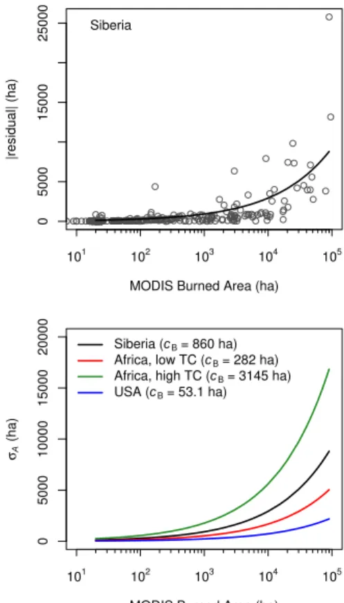
United States using ground truth maps produced manually from high resolution Land-sat imagery. An analysis of the residuals in MODIS vs. LandLand-sat burned areas showed that the variance in the measured area of an individual fire scar is approximately pro-portional to the area of the fire scar (Fig. 2). As the range of burn sizes examined in that study (approximately 0.1 ha to 300 000 ha) spans the range of burned area

possi-5

ble within a 0.5◦ GFED3 grid cell, we may use this result to conservatively model the uncertainty in our binned monthly burned area estimates. Thus

σ_A2(i ,t)₌cB(i)A(i ,t), (3)

where σ_A(i ,t) is the standard deviation of the monthly burned area estimate (here obtained by binning pixels of our 500-m burned area maps) and cB is the

“binned-10

burned-area uncertainty coe_fficient” for the grid cell at locationi. In having estimated the coefficient cB using validation data for individual burns (rather than total burned

area in a grid cell) we are not accounting for the potential canceling of errors due to the presence of multiple burns within the same grid cell, hence our description of this approach as a “conservative” model since it may tend to overestimate the actual

uncer-15

tainty. In extrapolating the results from the three validation regions we used the results for Siberia in BOAS and BONA, the results from the Western United States in TENA, and the results for Southern Africa in SHAF and NHAF, partitioned into low and high tree cover regions using the global VCF data set averaged to 0.5◦spatial resolution. In the remaining GFED regions we used the median value ofcB=571 ha.

20

3.3.2 Regression uncertainties

When using Eq. (1) to indirectly estimate monthly area burned we followed the ap-proach of Giglio et al. (2006b) and regressed the square of the residuals against monthly fire counts for each grid cell. The varianceσRpredicted by this supplementary

fit then provides an estimate of the regression uncertainty, i.e.,

25

(12)

BGD

6, 11577–11622, 2009

trends

L. Giglio et al.

Title Page

Tables Figures

◭ ◮

Back Close

Full Screen / Esc

where cR is the “regression variance coefficient” for the grid cell at location i. We

must also account for the inherent variance in the binned 500-m burned area training observations used in calibrating Eq. (1). We estimate this variance using Eq. (3), but with monthly burned areaA(i ,t) predicted using Eq. (1). Thus

σ_B2(i ,t)=cB(i)A(i ,t). (5)

5

The total one-standard-deviation (“one-sigma”) uncertainty estimate for all future pre-dictions is then the sum of the respective one-sigma uncertainties:

σ_A(i ,t)=σR(i ,t)+σB(i ,t) (6)

Here we do not add the respective uncertainties in quadrature as both terms on the right hand side of Eq. (6) are derived from monthly fire counts and are consequently

10

not independent.

When using Eq. (2) to indirectly estimate monthly burned area the procedure is iden-tical except that a separate regression variance coefficient is now associated with each terminal node of each regression tree, i.e.,

σ_R2(i ,t)₌cR,rNf(i ,t), (7)

15

where the coefficientcR,r is a function of the splitting variables in the regionr regres-sion tree.

3.4 Ancillary fire and burned area data layers

In addition to the gridded monthly burned area and uncertainty estimates described above, GFED3 provides additional ancillary data layers useful for modeling as well as

20

general use of the data set. These include: 1) the distribution of burned area within the grid cell as a function of fractional tree cover from the MODIS VCF product (Hansen et al., 2003), 2) the distribution of burned area within the grid cell across different MODIS land cover classes (Friedl et al., 2002), and 3) the fraction of burned area observed in organic peat (currently our peat map is limited to Borneo and Sumatra,

(13)

BGD

6, 11577–11622, 2009

trends

L. Giglio et al.

Title Page

Tables Figures

◭ ◮

Back Close

Full Screen / Esc

where peat fires are most prevalent). For the MODIS era we compiled these fields using our high quality 500-m MODIS burned area maps for each 0.5◦ grid cell; when these maps were not available (as during the pre-MODIS era) we compiled the fields based on the locations of all 1-km active fire pixels (2.5 km for VIRS) within each grid cell. Based on the utility of fire persistence for identifying deforestation fires, monthly

5

fire persistence was calculated using active fire observations as described in Giglio et al. (2006b) and provided in an additional ancillary data layer.

4 Results

4.1 Local regression

Equation (1) was fitted separately for each sensor to obtain the spatially-dependent

10

regression coefficientsα and β. Because small changes in the exponent β can pro-duce very large changes in the coefficient α (over several orders of magnitude), it is instructive to consider the special case in whichβ is constrained to unity. Under this constraint the coefficient α represents the effective burned area per fire pixel, and is directly comparable across all grid cells. For this special linear case we show the

co-15

efficientsα and the corresponding correlation for each sensor in Fig. 3. For all three sensors the general spatial pattern in the effective burned area per fire pixel reflects an increase inα with an increase in herbaceous vegetation fraction due to the lower densities and higher fire spread rates characteristic of dryer, herbaceous fuels (Sc-holes et al., 1996; van der Werf et al., 2003; Giglio et al., 2006b). A secondary (and

20

independent) feature applicable only to the ATSR sensor is a decrease inα at higher latitudes due to the latitudinal increase in the frequency of satellite overpasses. For the MODIS and VIRS sensors this feature is effectively absent since the gridded MODIS and VIRS fire products are corrected for this variation in overpass frequency character-istic of all polar-orbiting and precessing satellites. Additional factors a_ffectingαinclude

25

(14)

BGD

6, 11577–11622, 2009

trends

L. Giglio et al.

Title Page

Tables Figures

◭ ◮

Back Close

Full Screen / Esc

obscuration.

Comparing across platforms, the MODIS instrument consistently has the least burned area per fire pixel (lowestα) and the highest correlation between monthly fire counts and monthly burned area, while the ATSR-2/AATSR sensor consistently has the most burned area per fire pixel (highestα) and the lowest correlation. The VIRS

sen-5

sor in turn lies between these two extremes. This trend is a result of the lower relative sampling frequencies of the VIRS and ATSR sensors (Giglio et al., 2006b). Conse-quently, more burned area must be assigned to each fire pixel (thus raisingα), and the frequency of unobserved fires is greater (thus reducing the correlation) for these sensors. The impact on the GFED3 burned area data set will be larger uncertainties in

10

the pre-MODIS and especially the pre-VIRS time periods.

4.2 Regional regression trees

Regression trees were constructed for each sensor and each region. A representative example for each sensor is shown for the NH Africa region in Fig. 4. The number of terminal nodes in the Terra MODIS trees ranged from 9 (NHSA) to 16 (BONA, SHSA,

15

NHAF, and BOAS), and for the ATSR ranged from 5 (EURO, SHAF, and SEAS) to 8 (BONA, TENA, MIDE, BOAS, and AUST). For VIRS the largest tree (AUST) contained 16 terminal nodes. (The minimum VIRS tree size is not meaningful to compare be-cause the sensor provides only partial coverage in many extra-tropical regions.) Unlike GFED2, the wide range of sizes does not reflect differences in the quantity of

calibra-20

tion data available for each region, but rather the complexity of the relationship between burned area and fire counts (which is in turn influenced by the size of the region), and the strength of the association between these quantities. The significantly lower corre-lations observed in the tropics for the ATSR, for example, result in smaller trees simply because further splitting of terminal nodes yields no meaningful improvement in the

25

(15)

BGD

6, 11577–11622, 2009

trends

L. Giglio et al.

Title Page

Tables Figures

◭ ◮

Back Close

Full Screen / Esc

4.3 Pre-MODIS correction

As discussed above, both the VIRS and the ATSR provide substantially lower sampling rates compared to the Terra MODIS sensor. In the case of the ATSR this undersampling can be quite severe, and is further exacerbated by the fact that the sensor records only nighttime fires occurring well after the mid-afternoon peak in tropical fire activity

5

(Giglio, 2007). This leads to large numbers of grid cells in which active fires are never detected, yet which contain burned area. In this situation it is impossible for burned area to be allocated to such grid cells via Eq. (1) or (2), and the cumulative effect of such occurrences over large spatial and temporal scales is to underestimate the total area burned. To compensate for this e_ffect, we applied regional correction factors to our

10

monthly VIRS- and ATSR-based burned area estimates to achieve better consistency with our MODIS-based monthly estimates. We denote these factors byγ_r, where the subscriptr denotes the region. The corrected monthly burned area estimateA′(i ,t) in the grid cell at locationi during monthtis then

A′

(i ,t)₌γrA(i ,t), (8)

15

whereA(i ,t) is the uncorrected monthly burned area estimate predicted by Eqs. (1) or (2).

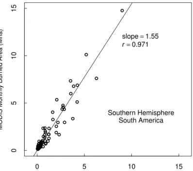
Correction factors were derived by linearly regressing the total monthly burned area derived from MODIS in each region against the corresponding total burned area esti-mated from VIRS and ATSR monthly fire counts, i.e.,

20

X

i∈r

A_MODIS(i ,t)=γ_rX

i∈r

A_VIRS(i ,t), (9)

where A_MODIS(i ,t) is the monthly burned area in each grid cell within region r and month t as derived from the binned 500-m MODIS burned area maps [or monthly MODIS fire counts and either Eqs. (1) or (2) when the 500-m maps are unavailable], andAVIRS(i ,t) is the corresponding uncorrected burned area in each grid cell as

esti-25

(16)

BGD

6, 11577–11622, 2009

trends

L. Giglio et al.

Title Page

Tables Figures

◭ ◮

Back Close

Full Screen / Esc

coefficients are similarly derived for the ATSR. The resulting coefficients γr are then used to correct the initial ATSR and VIRS burned area estimates in each grid cell through Eq. (8). An example regression for the ATSR is shown in Fig. 5. A complete list of regional correction factors is provided in Table 1.

It is important to keep in mind that the correction in Eq. (8) does not restore burned

5

area to those VIRS and ATSR zero-fire-count grid cells that cause the cumulative un-derestimation of burned area in the first place. The correction merely increases the area burned in grid cells already containing burned area, based on the average frac-tion of burned area that is missing (relative to MODIS) in each region. While far from perfect, we deemed this approach preferable to “painting in” missing burned area on

10

the basis of, e.g., a fire climatology.

In propagating uncertainties we must include the effect of the correction factor, in-cluding the uncertainty in the correction factor itself. The uncertainty in our corrected pre-MODIS monthly burned area estimates is then

σ_A′(i ,t)=γ_rA(i ,t)

"

_σ

A(i ,t)

A(i ,t) 2

+

σ

γ,r

γr 2#

1 2

, (10)

15

whereσγ,ris the uncertainty inγr. Here we have assumed that the uncertaintiesσA(i ,t) andσ_γ,r are random and independent, which is valid since inclusion of our VIRS- and ATSR-based burned area estimates in the GFED3 time series was restricted to the pre-MODIS era, hence no pre-MODIS observations were used in fitting Eq. (9).

4.4 Multi-year burned area estimates

20

We used the hybrid approach described in Sect. 3 with the correction described in Sect. 4.3 to produce monthly burned area estimates spanning July 1996 through mid-2009. As the spatial coverage of our ATSR- and VIRS-based estimates overlap in the tropics and sub-tropics, we used the following scheme to merge the estimates from these sensors during the pre-MODIS era. From January 1998 (the first full calendar

(17)

BGD

6, 11577–11622, 2009

trends

L. Giglio et al.

Title Page

Tables Figures

◭ ◮

Back Close

Full Screen / Esc

month of VIRS data) through October 2000 (the last month of the pre-MODIS era) the choice of sensor was made independently for each region based on sensor coverage and the quality of the fit in Eq. (9). Under these criteria, ATSR fire counts were used in all high-latitude regions as well as CEAM, SHAF, CEAS, and EQAS, and VIRS fire counts were used in NHSA, SHSA, NHAF, and AUST. In the remaining regions data

5

from the two sensors were merged, with VIRS observations having precedence when available. Prior to January 1998 the GFED3 burned area time series was produced exclusively from ATSR observations.

Regional monthly burned area time series are shown in Figs. 6 and 7. Here the different colors indicate the proportion of the monthly area burned contributed by each

10

of the di_fferent sensors and methodologies used to produce the multi-year data set. In Fig. 8 we show the spatially explicit 1997–2008 mean annual area burned and the associated uncertainties. It is important to note that the magnitude of the uncertainties in our GFED3 burned area data set are not uniform over time; they are smallest during the MODIS era, when the majority of the burned area estimates are obtained directly

15

from our 500-m burned area maps, larger during the 1998–2000 VIRS/ATSR overlap period, and larger still during the 1996–1997 ATSR-only era. For example, the 1997 global mean burned area uncertainty is nearly seven times larger than the 2007 global mean burned area uncertainty, despite comparable total area burned in both years.

Following Giglio et al. (2006a), we calculated two climatological fields from our

20

monthly burned area estimates as part of our analysis. These were: 1) the seasonal peak in fire activity, defined as the calendar month having the greatest area burned (Fig. 9a), and 2) the 12-month lagged autocorrelation of the full 1996–2008 monthly burned area time series (Fig. 9b), which provides a spatially-explicit measure of the interannual variability and periodicity of fire activity. The seasonal peak shows very

25

(18)

tempo-BGD

6, 11577–11622, 2009

trends

L. Giglio et al.

Title Page

Tables Figures

◭ ◮

Back Close

Full Screen / Esc

ral autocorrelation tends to occur in many parts of the tropics, with the highest values occuring in African savannas, and lower autocorrelation (i.e., greater interannual vari-ability) occurring in regions prone to sporadic burning, including Australia, the United States, and boreal forests of both Asia and North America.

In Table 2 and Fig. 10 we summarize the annual area burned within each GFED

5

region. The most extensive area burned consistently occurred in Northern Hemisphere (NH) and Southern Hemisphere (SH) Africa, with∼250 Mha burned on the continent

annually. This represents on average about 70% of the global area burned each year. The remaining 30% is composed primarily of area burned in Australia, followed by SH South America and Central Asia.

10

At 13 years the duration of our GFED3 data set is still too short to reliably iden-tify regional burned area trends, particularly in light of the major 1997–1998 El-Ni ˜no Southern Oscillation (ENSO) event at the beginning of the time series. Considering only the most obvious trends, however, we note the following with respect to burned area: 1) a very gradual increase (+1.5 Mha yr−1) in SH Africa since 2002; 2) an

incon-15

sistent though comparatively rapid decrease (−6 Mha yr−1) in Australia since 2001; and 3) a gradual decrease (−8 Mha yr−1) in global burned area since 1998, which beginning

in 2001 is primarily a result of the rapid decrease in Australia.

With respect to the impact of ENSO events on fire activity during the GFED3 era, we note a significant association between the Southern Oscillation Index (SOI) and

20

area burned in Equatorial Asia and Australia (Fig. 11). In Equatorial Asia the impact of ENSO activity (as measured by negative values of the SOI) was both positive and im-mediate, with greater burned occurring during ENSO events. This is consistent with the earlier and more detailed analysis of Fuller and Murphy (2006), who reported a strong inverse correlation between the SOI and five years of monthly ATSR fire counts in

25

(19)

BGD

6, 11577–11622, 2009

trends

L. Giglio et al.

Title Page

Tables Figures

◭ ◮

Back Close

Full Screen / Esc

Werf et al., 2008). We found significant (though somewhat weaker) associations in sev-eral other regions, in particular CEAM, TENA, and BOAS, with burned area typically lagging the SOI by five to eight months.

5 Comparison with other satellite-based burned area products

We compared our global burned area data set to the L3JRC, Collection 5 MODIS

5

(MCD45A1), and GLOBCARBON burned area products, as well as the GFED2 burned area data set. We binned the L3JRC and MCD45A1 products to monthly temporal and 0.5◦ spatial resolution to facilitate the comparison. For each data set we calculated the total area burned annually on a regional basis (Fig. 10) and the 2001–2006 mean annual area burned (Fig. 12).

10

5.1 Comparison with GFED2

The annual time series in Fig. 10 indicate that while GFED3 shows only a relatively modest (∼10%) increase in worldwide area burned each year over GFED2, the dif-ference in some regions is substantially larger. The magnitude of these differences can be seen more clearly in Fig. 13, which shows the relative change in mean burned

15

area from GFED2 to GFED3. While the relative change is greatest in the Middle East and Europe, the area burned in these regions represents less than 0.5% of the total area burned worldwide each year and is in this sense comparatively unimportant at the global scale.

Of greater significance is the ∼60% increase in annual burned area in Southern

20

Hemisphere Africa (SHAF), where approximately one third of the total area burned worldwide occurs each year. Based on a separate analysis (not shown) we deter-mined that about 30% of this difference was due to significant omission errors in some of the 500-m burned area training maps used to produce GFED2, where the impact of these errors was amplified by the very small number of training maps available at

(20)

BGD

6, 11577–11622, 2009

trends

L. Giglio et al.

Title Page

Tables Figures

◭ ◮

Back Close

Full Screen / Esc

the time. This lack of training data was ultimately responsible for the remaining 70% of the di_fference as well. This can be seen from Fig. 14, which shows the frequency distribution of the effective burned area per fire pixel (α) for all grid cells within SHAF for the constrained local regression (β=1) described in Sect. 4.1. (Here we consider the constrained case as it permits a direct comparison with GFED2.) Superimposed

5

on the continuous frequency distribution (which qualitatively resembles an exponential distribution) are the discrete values ofα (shown as black vertical lines, with height in-dicating frequency) in each of the seven terminal nodes of the GFED2 SHAF regional regression tree (Fig. 14 inset). Of interest here is the difference in the general shape of each distribution, as well as the significant gaps in the discrete case. Had the

re-10

gression tree been grown with a su_fficiently large training sample, the two distributions would be in much better agreement, with similar shapes and with the discrete values ofαin the (now large) set of terminal nodes spaced much more densely over the con-tinuous distribution. Being limited in size by the small quantity of training data available at the time, however, the SHAF regression tree is too small to adequately represent

15

the entire range of α needed to accurately estimate burned area, with the following consequences: In the 23% of grid cells for which GFED3 has a value ofα below the GFED2 minimum of 1.01 km2/pixel, GFED2 will overestimate burned area. The termi-nal node containing this minimum happens to be the most common destination for the highest tree cover grid cells found in SHAF, thus GFED2 tends to allocate this excess

20

burned area to wooded areas within this region. Conversely, the small number of ter-minal nodes located in the upper half of the continuous distribution leads to a deficit of burned area in the less wooded areas of SHAF, thus in this region GFED2 routinely underestimates the extent of savanna fires.

This same paucity of training data limits the fidelity of the GFED2 regression trees

25

(21)

BGD

6, 11577–11622, 2009

trends

L. Giglio et al.

Title Page

Tables Figures

◭ ◮

Back Close

Full Screen / Esc

exponential distributions obtained through local regression.

To help assess the extent of the improvements incorporated into GFED3, we com-pared burned area estimates from both GFED2 and GFED3 to independent estimates compiled by the Canadian Interagency Forest Fire Centre (CIFFC) and the National Interagency Fire Center (NIFC). The CIFFC provides yearly burned area totals for

5

nine Canadian provinces (British Columbia, Alberta, Manitoba, Newfoundland and Labrador, Northwest Territories, Ontario, Quebec Saskatchewan, and the Yukon Terri-tories). Plots of GFED versus CIFFC burned area (Fig. 15, top) show the significantly improved agreement attained with GFED3 during both the MODIS and pre-MODIS eras. Improvement is also seen in the comparison with NIFC estimates for the United

10

States (Fig. 15, bottom), particularly during the pre-MODIS era.

5.2 Comparison with the MCD45A1, L3JRC, and GLOBCARBON burned area

data sets

To facilitate our comparison with the MCD45A1, L3JRC, and GLOBCARBON prod-ucts, we analyzed spatially explicit differences during 2001–2006 when data from all

15

four products was available (Fig. 16). Focusing first on the L3JRC product, the burned area reported in this data set is consistently many times larger than both the GFED3 and MCD45A1 products in seven regions (Boreal North America, Temperate North America, Central America, Europe, Middle East, Boreal Asia, and Central Asia) and, conversely, consistently about half as large in NH Africa and two thirds as large in SH

20

Africa. The large surplus in seven regions is alarming since the validation performed by Tansey et al. (2008) using 72 Landsat-based reference maps revealed a substantial underestimation of area burned in the L3JRC product (by roughly a factor of two) in all land cover classes they considered with the exception of needle-leaved deciduous forest. This finding might seem to suggest that the GFED3 and MCD45A1 burned area

25

(22)

BGD

6, 11577–11622, 2009

trends

L. Giglio et al.

Title Page

Tables Figures

◭ ◮

Back Close

Full Screen / Esc

(AFS), we conclude that the L3JRC product is significantly overestimating burned area in at least North America (Fig. 17). We note also that while the GFED3 and MCD45A1 annual totals are highly correlated with the independent North American estimates, the L3JRC totals are either uncorrelated or negatively correlated with the indepen-dent estimates. These results are consistent with the findings of Chang and Song

5

(2009) in a recent intercomparison of the L3JRC and MODIS products, although the zero-intercept regression constraint used by the authors inadvertently obscures those instances in which the L3JRC burned areas and the national statistics are inversely related. The L3JRC product also often reports burned area in arid regions containing little burnable vegetation. The proximity of these regions to “pure” deserts suggests

10

that these burned areas might actually be false alarms limited in extent by a static desert mask.

The GLOBCARBON product strongly resembles the L3JRC product, with a similar spatial distribution of burned area, but generally lower magnitude. Like the L3JRC product, it appears to significantly overestimate burned area in the continental United

15

States and Canada, and shares the same poor correlation with independent estimates (Fig. 17). A major di_fference between the two products occurs in Central America, however, where the GLOBCARBON totals are comparable to those of GFED3 and MCD45A1, and the L3JRC totals are about three times larger. In SH Africa, GLOB-CARBON consistently reported the least burned area of all data sets, a result that

20

initially appears to be inconsistent with the Southern Africa validation study of Roy and Boschetti (2009). Based on an analysis of 11 Landsat scenes, the authors found that the L3JRC and GLOBCARBON products successfully mapped 14% and 60%, respec-tively, of the true area burned. Based on this result, one would expect the burned area reported in SHAF to be considerably higher for GLOBCARBON than for the L3JRC

25

(23)

BGD

6, 11577–11622, 2009

trends

L. Giglio et al.

Title Page

Tables Figures

◭ ◮

Back Close

Full Screen / Esc

Africa totals were compiled over a much larger area than the Roy and Boschetti study region (by a factor of about 35), and consequently include very large areas spanning some climatic zones not considered in their analysis for which their results may not be representative.

Focusing next on the GFED3 and MCD45A1 data sets, the annual areas burned for

5

these products have much greater consistency in most regions. We note, however, that the former tends to allocate more burned area along gradients between bare ground and herbaceous vegetation, while the latter tends to allocate more burned area in crop-land. Despite having comparable annual totals in NH and SH Africa, the GFED3 and MCD45A1 products show substantial spatial differences in both regions. Aside from

10

GFED3 again allocating more burned area along bare-herbaceous gradients, the spa-tial trends with respect to vegetation are much less consistent in Africa than elsewhere. The EQAS region warrants particular attention because here GFED3 consistently reports much higher annual burned area totals than either the MCD45A1, L3JRC, or GLOBCARBON products (which are relatively consistent in this case). For this region

15

the “surplus” GFED3 annual burned area is typically 1–2 Mha. The relative discrepancy in EQAS exceeds 100% and is worrisome because comparable relative discrepancies will propagate into any higher-level modeling effort (such as emissions modeling) mak-ing use of the different products. To help explain this discrepancy, we examined daily MODIS surface reflectance imagery from 2002 and 2006 for several MODIS tiles in

20

the region. While extensive burning could be sporadically identified in the imagery, the combination of persistent cloud cover and apparently overly-aggressive cloud and aerosol filtering used in generating the MCD45A1 product restricted mapping to a small fraction of the actual fire season. This was especially true in 2006, when anomalously high fire activity in Southern Borneo peaked unusually late in the fire season and

subse-25

(24)

BGD

6, 11577–11622, 2009

trends

L. Giglio et al.

Title Page

Tables Figures

◭ ◮

Back Close

Full Screen / Esc

to cloud and aerosol contamination, the larger number of (potentially noisier) observa-tions available for use translates into fewer unmapped pixels. These same issues of persistent cloud cover and aerosol contamination are likely to contribute to the rela-tively low burned areas reported for EQAS in the L3JRC and GLOBCARBON products as well.

5

6 Conclusions

We used a combination of active fire observations from multiple satellites, 500-m MODIS burned area maps, local regression, and regional regression trees to produce a hybrid, global, monthly burned area data set from July 1996 through mid-2009. An-nual totals derived from these data showed good agreement with independent anAn-nual

10

estimates available for Canada and the United States (both nationally and in the state of Alaska). Using these data we estimated the global annual burned area for the years 1997–2008 to vary between 330 and 431 Mha, with the maximum occurring in 1998 and the minimum in 2008. The most extensive burning consistently occurred in Africa, with∼250 Mha burned on the continent each year. This represents on average about

15

70% of the total area burned worldwide annually.

By considering the 12-month lagged autocorrelation of the burned area time series, we found that the lowest interannual variability in area burned occurred in the savannas of Southern- and Northern-Hemisphere Africa. Regions of high interannual variability included Australia, the United States, and boreal forests of both Asia and North

Amer-20

ica, where much more sporadic burning is the norm. These results are consistent with earlier efforts to characterize global fire activity using active fire data obtained from satellite-based sensors.

We compared our global burned area data set to the L3JRC, MODIS MCD45A1, and GLOBCARBON burned area products, as well as the GFED2 burned area data

25

(25)

BGD

6, 11577–11622, 2009

trends

L. Giglio et al.

Title Page

Tables Figures

◭ ◮

Back Close

Full Screen / Esc

much lower than the GFED3 and MCD45A1 products in NH and SH Africa. Using in-dependent national burned area statistics, we showed that the L3JRC product appears to be consistently overestimating the area burned in the continental United States and Canada each year by a factor of three to ten. The GLOBCARBON product most closely resembled the L3JRC product, with a similar spatial distribution of burned area but

5

generally lower magnitude. Similarly, our GFED3 data set most closely resembled the MCD45A1 data set, both in terms of the spatial distribution of burned area, as well as the annual area burned in most regions.

Acknowledgements. We thank Mingquan Mu for helpful technical discussions. Both the ATSR World Fire Atlas and the GLOBCARBON burned area product are made available through 10

the European Space Agency. This work was supported by NASA grants NNX08AF64G,

NNX08AE97A, NNX08AL03G, and NNX08AQ04G.

References

Arino, O. and Rosaz, J.-M.: 1997 and 1998 world ATSR fire atlas using ERS-2 ATSR-2 data, in: Proceedings of the Joint Fire Science Conference and Workshop, edited by Neuenschwan-15

der, L. F., Ryan, K. C., and Gollberg, G. E., vol. 1, University of Idaho and the International Association of Wildland Fire, Boise, Idaho, 177–182, 1999. 11581

Breiman, L., Friedman, J. A., Olshen, R. A., and Stone, C. J.: Classification and Regression Trees, Chapman and Hall/CRC, Boca Raton, 1984. 11583

Chang, D. and Song, Y.: Comparison of L3JRC and MODIS global burned area products from 20

2000 to 2007, J. Geophys. Res., 114, D16106, doi:10.1029/2008JD011361, 2009. 11598 Friedl, M. A., McIver, D. K., Hodges, J. C. F., Zhang, X. Y., Muchoney, D., Strahler, A. H.,

Wood-cock, C. E., Gopal, S., Schneider, A., Cooper, A., Baccini, A., Gao, F., and Schaaf, C.: Global land cover mapping from MODIS: algorithms and early results, Remote Sens. Environ., 83, 287–302, 2002. 11580, 11588

25

Fuller, D. O. and Murphy, K.: The ENSO-fire dynamic in insular southeast Asia, Climatic Change, 74, 435–455, 2006. 11594

(26)

BGD

6, 11577–11622, 2009

trends

L. Giglio et al.

Title Page

Tables Figures

◭ ◮

Back Close

Full Screen / Esc

Giglio, L., Kendall, J. D., and Mack, R.: A multi-year active fire data set for the tropics derived from the TRMM VIRS, Int. J. Remote Sens., 24, 4505–4525, 2003. 11581

Giglio, L., Csiszar, I., and Justice, C. O.: Global distribution and seasonality of active fires as observed with the terra and aqua MODIS sensors, J. Geophys. Res., 111, G02016, doi:10.1029/2005JG000142, 2006a. 11593

5

Giglio, L., van der Werf, G. R., Randerson, J. T., Collatz, G. J., and Kasibhatla, P.: Global estimation of burned area using MODIS active fire observations, Atmos. Chem. Phys., 6, 957–974, 2006b,

http://www.atmos-chem-phys.net/6/957/2006/. 11579, 11580, 11581, 11587, 11589, 11590, 11606, 11609

10

Giglio, L., Loboda, T., Roy, D. P., Quayle, B., and Justice, C. O.: An active-fire based burned area mapping algorithm for the MODIS sensor, Remote Sens. Environ., 113, 408–420, doi:10.1016/j.rse.2008.10.006, 2009. 11580, 11581, 11582, 11586, 11607

Hansen, M. C., DeFries, R. S., Townshend, J. R. G., Carroll, M., Dimiceli, C., and Sohlberg, R. A.: Global percent tree cover at a spatial resolution of 500 meters: first results of 15

the MODIS vegetation continuous fields algorithm, Earth Interact., 7(10), doi:10.1175/1087-3562, 2003. 11584, 11588

Justice, C. O., Giglio, L., Korontzi, S., Owens, J., Morisette, J. T., Roy, D., Descloitres, J., Al-leaume, S., Petitcolin, F., and Kaufman, Y.: The MODIS fire products, Remote Sens. Environ., 83, 244–262, 2002. 11580

20

Langmann, B., Duncan, B., Textor, C., Trentmann, J., and van der Werf, G. R.: Vegetation fire emissions and their impact on air pollution and climate, Atmos. Environ., 43, 107–116, doi:10.1016/j.atmosenv.2008.09.047, 2009. 11579

Plummer, S., Arino, O., Simon, M., and Steffen, W.: Establishing an earth observation product

service for the terrestrial carbon community: the GLOBCARBON initiative, Mitigation and 25

Adaptation Strategies for Global Change, 11, 97–11, 2006. 11579

Roy, D. P. and Boschetti, L.: Southern Africa validation of the MODIS, L3JRC,

and GlobCarbon burned-area products, IEEE T. Geosci. Remote, 47, 1032–1044, doi:10.1109/TGRS.2008.2009000, 2009. 11598

Roy, D. P., Jin, Y., Lewis, P. E., and Justice, C. O.: Prototyping a global algorithm for systematic 30

fire-affected area mapping using MODIS time series data, Remote Sens. Environ., 97, 137–

162, 2005. 11599

(27)

prod-BGD

6, 11577–11622, 2009

trends

L. Giglio et al.

Title Page

Tables Figures

◭ ◮

Back Close

Full Screen / Esc

uct – global evaluation by comparison with the MODIS active fire product, Remote Sens. Environ., 112, 3690–3707, doi:10.1016/j.rse.2008.05.013, 2008. 11579

Scholes, R. J., Kendall, J. D., and Justice, C. O.: The quantity of biomass burned in Southern Africa, J. Geophys. Res., 101, 23667–23676, 1996. 11589

Tansey, K., Gr ´egoire, J.-M., Stroppiana, D., Sousa, A., Silva, J., Pereira, J. M. C., Boschetti, L., 5

Maggi, M., Brivio, P. A., Fraser, R., Flasse, S., Ershov, D., Binaghi, E., Graetz, D., and Pe-duzzi, P.: Vegetation burning in the year 2000: global burned area estimates from SPOT VEGETATION data, J. Geophys. Res., 109, D14S03, doi:10.1029/2003JD003598, 2004. 11579

Tansey, K., Gr ´egoire, J.-M., Defourny, P., Leigh, R., Pekel, J.-F., van Bogaert, E., and 10

Bartholom ´e, E.: A new, global, multi-annual (2000–2007) burnt area product at 1 km resolu-tion, Geophys. Res. Lett., 35, L011401, doi:10.1029/2007GL031567, 2008. 11579, 11597 van der Werf, G. R., Randerson, J. T., Collatz, G. J., and Giglio, L.: Carbon emissions from fires

in tropical and subtropical ecosystems, Glob. Change Biol., 9, 547–562, 2003. 11589 van der Werf, G. R., Randerson, J. T., Giglio, L., Collatz, G. J., Kasibhatla, P. S., and Arel-15

lano Jr., A. F.: Interannual variability in global biomass burning emissions from 1997 to 2004, Atmos. Chem. Phys., 6, 3423–3441, 2006,

http://www.atmos-chem-phys.net/6/3423/2006/. 11579, 11606

van der Werf, G. R., Randerson, J. T., Giglio, L., Gobron, N., and Dolman, A. J.: Climate controls on the variability of fires in the tropics and subtropics, Global Biogeochem. Cy., 22, GB3028, 20

doi:10.1029/2007GB003122, 2008. 11594

Vermote, E. F. and Justice, N. Z. E. S. C. O.: Operational atmospheric correction of the MODIS data in the visible to middle infrared: first results, Remote Sens. Environ., 83, 97–111, 2002. 11580

Wolfe, R. E., Roy, D. P., and Vermote, E.: MODIS land data storage, gridding, and compositing 25

(28)

BGD

6, 11577–11622, 2009

trends

L. Giglio et al.

Title Page

Tables Figures

◭ ◮

Back Close

Full Screen / Esc

Table 1. Monthly ATSR and VIRS burned area correction factors (γ_r) and linear correlation

coefficients (r).

ATSR VIRS

Region γ_r r γ_r r

Boreal North America 1.35 0.941 – –

Temperate North America 1.52 0.953 1.50 0.902

Central America 1.39 0.965 1.35 0.954

NH South America 1.42 0.856 1.22 0.890

SH South America 1.55 0.971 1.25 0.972

Europe 1.75 0.952 – –

Middle East 1.30 0.908 2.38 0.841

NH Africa 1.84 0.905 1.14 0.988

SH Africa 2.13 0.972 1.11 0.961

Boreal Asia 1.36 0.889 – –

Central Asia 1.70 0.980 – –

Southeast Asia 1.39 0.775 1.45 0.921

Equatorial Asia 1.40 0.961 1.43 0.966

(29)

BGD

6, 11577–11622, 2009

trends

L. Giglio et al.

Title Page

Tables Figures

◭ ◮

Back Close

Full Screen / Esc

Table 2.1997–2008 estimated annual regional and worldwide area burned.

Area Burned (×104km2=Mha)

Region 1997 1998 1999 2000 2001 2002 2003 2004 2005 2006 2007 2008 Mean

BONA 0.9 4.5 1.5 0.7 0.3 3.2 2.0 5.0 2.9 1.9 1.5 1.4 2.2

TENA 0.5 1.1 1.8 2.2 1.2 1.4 1.3 0.7 1.7 2.4 2.7 1.5 1.5

CEAM 0.9 3.2 1.3 1.7 1.0 1.0 1.7 0.8 1.9 1.3 1.1 1.2 1.4

NHSA 1.7 2.8 2.0 2.4 2.0 1.1 3.3 3.2 1.8 1.5 2.5 1.8 2.2

SHSA 16.0 38.9 30.9 15.8 19.4 21.3 16.1 18.7 22.1 12.5 33.8 13.4 21.6

EURO 0.4 0.8 0.6 1.2 1.1 0.4 0.9 0.5 0.6 0.5 1.0 0.5 0.7

MIDE 0.6 0.9 0.8 0.6 1.2 1.0 0.9 0.8 0.7 0.9 1.2 0.6 0.9

NHAF 152.4 148.7 143.5 145.9 114.4 126.1 128.0 116.4 139.9 115.2 123.4 117.7 131.0

SHAF 111.6 153.1 123.1 118.3 117.3 113.9 126.6 127.1 134.1 122.2 124.2 131.5 125.2

BOAS 3.1 12.9 4.7 7.2 5.8 8.1 15.9 1.6 2.8 4.3 3.2 12.0 6.8

CEAS 17.4 14.6 8.1 11.0 15.0 25.0 12.8 15.6 15.1 17.5 12.5 14.0 14.9

SEAS 3.9 7.9 9.5 4.5 4.5 7.7 6.3 10.7 7.1 5.9 9.9 7.0 7.1

EQAS 9.4 2.6 0.6 0.4 0.7 2.4 0.8 1.2 1.1 2.7 0.5 0.4 1.9

AUST 40.5 39.0 80.2 81.7 88.3 73.1 29.0 60.4 24.9 53.1 48.7 26.6 53.8

(30)

BGD

6, 11577–11622, 2009

trends

L. Giglio et al.

Title Page

Tables Figures

◭ ◮

Back Close

Full Screen / Esc

Fig. 1. Map of the 14 regions used in this study, after Giglio et al. (2006b) and van der Werf

(31)

BGD

6, 11577–11622, 2009

trends

L. Giglio et al.

Title Page

Tables Figures

◭ ◮

Back Close

Full Screen / Esc

0

5000

15000

25000

MODIS Burned Area (ha)

|residual| (ha)

101 102 103 104 105 Siberia

0

5000

10000

15000

20000

MODIS Burned Area (ha) σA

(ha)

101 102 103 104 105 Siberia (cB = 860 ha)

Africa, low TC (cB = 282 ha)

Africa, high TC (cB = 3145 ha)

USA (cB = 53.1 ha)

Fig. 2. Top: example of fitted residuals from Giglio et al. (2009) Siberian validation data.

(32)

BGD

6, 11577–11622, 2009

trends

L. Giglio et al.

Title Page

Tables Figures

◭ ◮

Back Close

Full Screen / Esc

(a) ₀ ₁ (km₂ ₃ ₄ ₅

2_pixel-1₎

(b) _0.0 _0.2 _0.4 _0.6 _0.8 _1.0

(c) ₀ ₅ ₁₀(km ₁₅ ₂₀ ₂₅ ₃₀

2_pixel-1₎

(d) _0.0 _0.2 _0.4 _0.6 _0.8 _1.0

(e) ₀ ₁₀ (km₂₀ ₃₀ ₄₀ ₅₀

2_pixel-1₎

(f) _0.0 _0.2 _0.4 _0.6 _0.8 _1.0

ATSR VIRS Terra MODIS

Fig. 3. Effective burned area per fire pixel (left column) and corresponding linear correlation

(right column) for the constrained linear case (β=1) for the Terra MODIS(a, b), VIRS(c, d)and

ATSR(e, f)sensors. Note di_fferent scales used in (a), (c), and (e). The spatial coverage of the

VIRS is restricted to within approximately 38◦

(33)

BGD

6, 11577–11622, 2009

trends

L. Giglio et al.

Title Page

Tables Figures

◭ ◮

Back Close

Full Screen / Esc

Fig. 4. Example of regression trees relating monthly fire counts to monthly burned area

ob-tained for the Terra MODIS, VIRS, and ATSR sensors in the Northern Hemisphere Africa re-gion. The left fork is taken when the condition at a split is satisfied. The upper and lower

numbers in each terminal node (leaf) are the respective values of the parametersα_r (km2) and

β_r appearing in Eq. (2) for the node. As in Giglio et al. (2006b), the subscript “f” has been

dropped from the splitting variablesT_f (percent tree cover),H_f (percent herbaceous cover),B_f

(34)