doi:10.5194/bg-13-3717-2016
© Author(s) 2016. CC Attribution 3.0 License.
Biomass burning fuel consumption dynamics in the tropics and
subtropics assessed from satellite
Niels Andela1,2, Guido R. van der Werf1, Johannes W. Kaiser3, Thijs T. van Leeuwen4,5,6, Martin J. Wooster7,8, and Caroline E. R. Lehmann9
1Faculty of Earth and Life Sciences, VU University, Amsterdam, the Netherlands
2Biospheric Sciences Laboratory, NASA Goddard Space Flight Center, Greenbelt, MD 20771, USA 3Max-Planck-Institut für Chemie, Mainz, Germany
4SRON Netherlands Institute for Space Research, Utrecht, the Netherlands 5Institute for Marine and Atmospheric Research Utrecht, Utrecht, the Netherlands
6VanderSat B.V., Space Business Park, Huygensstraat 34, 2201 DK, Noordwijk, the Netherlands
7King’s College London, Environmental Monitoring and Modelling Research Group, Department of Geography,
London, WC2R 2LS, UK
8NERC National Centre for Earth Observation (NCEO), UK
9School of GeoSciences, University of Edinburgh, Edinburgh, EH9 3JN, UK
Correspondence to:Niels Andela ([email protected])
Received: 13 November 2015 – Published in Biogeosciences Discuss.: 18 January 2016 Revised: 25 May 2016 – Accepted: 1 June 2016 – Published: 28 June 2016
Abstract. Landscape fires occur on a large scale in (sub)tropical savannas and grasslands, affecting ecosystem dynamics, regional air quality and concentrations of atmo-spheric trace gasses. Fuel consumption per unit of area burned is an important but poorly constrained parameter in fire emission modelling. We combined satellite-derived burned area with fire radiative power (FRP) data to derive fuel consumption estimates for land cover types with low tree cover in South America, Sub-Saharan Africa, and Aus-tralia. We developed a new approach to estimate fuel con-sumption, based on FRP data from the polar-orbiting Moder-ate Resolution Imaging Spectroradiometer (MODIS) and the geostationary Spinning Enhanced Visible and Infrared Im-ager (SEVIRI) in combination with MODIS burned-area es-timates. The fuel consumption estimates based on the geosta-tionary and polar-orbiting instruments showed good agree-ment in terms of spatial patterns. We used field measure-ments of fuel consumption to constrain our results, but the large variation in fuel consumption in both space and time complicated this comparison and absolute fuel consumption estimates remained more uncertain. Spatial patterns in fuel consumption could be partly explained by vegetation pro-ductivity and fire return periods. In South America, most
studies especially designed to validate satellite-based prod-ucts, or airborne remote sensing, may further improve confi-dence in the absolute fuel consumption estimates which are quickly becoming the weakest link in fire emission estimates.
1 Introduction
Landscape fires play an important role in many ecosys-tems across the globe, with (sub)tropical savannas of inter-mediate productivity being most frequently burned (Bow-man et al., 2009). Within those (sub)tropical ecosystems, hu-mans are responsible for most of the ignitions and fires have been actively managed for thousands of years (Archibald et al., 2010, 2012; Stott, 2000), partly aided by the vege-tation traits of these regions which make them inherently flammable (Archibald et al., 2009). Landscape fires promote open-canopy grassy vegetation over closed canopy woody vegetation (Bond et al., 2005; Lehmann et al., 2011; Sc-holes and Archer, 1997), providing competitive advantages to grassy rather than woody species in frequently burning landscapes (Sankaran et al., 2008). This fire-driven tree– grass competition is further affected by the occurrence of different vegetation traits on the continents (Lehmann et al., 2014; Moncrieff et al., 2014; Staver et al., 2011). Due to the large scale at which biomass burning occurs, inter-annual variability in landscape fires is directly related to (green-house) gas concentrations in the atmosphere (Langenfelds et al., 2002) and affects regional air quality (Aouizerats et al., 2015; Crutzen et al., 1979; Langmann et al., 2009; Tur-quety et al., 2009). Fire regimes and fire management vary widely across (sub)tropical regions (Archibald et al., 2013), while ongoing socio-economic developments are expected to increasingly affect landscape fires and vegetation patterns during the coming century (Andela and van der Werf, 2014; Chen et al., 2013; Grégoire et al., 2013). Fuel consump-tion per unit area burned (kg m−2), hereafter called fuel con-sumption for brevity, is a key indicator of the consequences of changing management practices, vegetation characteris-tics and climate on fire regimes, as well as a key parameter required in fire emission estimates. Yet, spatiotemporal dy-namics of fuel consumption on a continental scale remain largely unmeasured and poorly understood (van Leeuwen et al., 2014).
With global annual burned area exceeding the size of In-dia (Giglio et al., 2013) or even the European Union (Ran-derson et al., 2012), satellite remote sensing is an important source of data to understand the spatiotemporal dynamics of fire. Over the last decade, several new satellite observing sys-tems have become operational, greatly improving our under-standing of fire dynamics and fire emission estimates. For example, vegetation productivity (Running et al., 2004) and fire return periods (Archibald et al., 2013) can now be es-timated using satellite imagery and data. Broadly speaking,
two types of satellite datasets are available to study fire dy-namics. These are satellite-derived estimates of burned area that are based on changes in surface reflectance over time (Giglio et al., 2006b, 2013) and active fire observations often accompanied by information on fire radiative power (FRP; Giglio et al., 2006a; Roberts and Wooster, 2008).
Both data types have advantages and disadvantages for the purpose of estimating fire emissions. Burned area remains visible for several days to months after the fire occurred, al-lowing observations of fires that were obscured by clouds during the satellite overpass, as long as cloud cover is not too persistent (Roy et al., 2008). However, small fires are generally not detected by the burned-area algorithm (Ran-derson et al., 2012) and fuel consumption has to be modelled if burned area is used to calculate emissions (van der Werf et al., 2010). Active fire observations, on the other hand, often include FRP associated with the detected fire, which can be used to estimate fire radiative energy (FRE), which is directly related to dry matter burned (Wooster et al., 2005). When FRP data of geostationary instruments are used, the full fire diurnal cycle is observed and FRE and dry matter burned can be estimated by integrating the FRP observations over time (Roberts et al., 2005). However, geostationary satellites are located relatively far from the Earth and therefore have a rela-tively coarse pixel size. Consequently, fires with low FRP fall below their detection threshold (Freeborn et al., 2009). Polar-orbiting instruments, like the Moderate Resolution Imaging Spectroradiometer (MODIS), are located closer to the Earth and therefore have a higher spatial resolution and sensitiv-ity to fires with low FRP. However, with approximately four daily observations under ideal conditions, the MODIS instru-ments provide relatively poor sampling of the fire diurnal cy-cle (Ellicott et al., 2009; Freeborn et al., 2011; Vermote et al., 2009). On top of the orbit-specific limitations, active fire ob-servations from both polar-orbiting and geostationary instru-ments are sensitive to cloud cover, and radiation of surface fires may be partly obscured by tree cover (Freeborn et al., 2014a).
der Werf et al., 2010). The satellite-derived fuel consumption estimates of Roberts et al. (2011) were considerably lower than the ones from GFED in savanna regions, which may partly be explained by the low sensitivity of the SEVIRI in-strument to small fires and an overestimate by GFED3. How-ever, spatial patterns were also different, indicating that such methods can provide new insights into the distribution of fuel consumption and of fuel build-up processes.
The objective of this study is to gain further insights into the spatial distribution and drivers of fuel consumption. Initially, fuel consumption is estimated across Sub-Saharan Africa by building upon the previous work of Roberts et al. (2009, 2011) that combined active fire FRP data from the geostationary SEVIRI instrument with burned-area data from MODIS. We used a similar approach, but with longer time series (2010–2014), in an attempt to provide more statisti-cally representative fuel consumption estimates, particularly in less frequently burning grid cells. Then we used a simi-lar method but now based on MODIS FRP data to expand our study region to include South America and Australia, in addition to Sub-Saharan Africa. In situ fuel consump-tion observaconsump-tions were used to calibrate the MODIS-derived fuel consumption estimates to match field-measured values. Because FRP observations may be partly obscured by tree cover (Freeborn et al., 2014a), we limited our study to low tree cover land cover classes. Results were compared to the SEVIRI-derived fuel consumption estimates and the estimate derived using the biochemical GFED modelling framework. Finally, we used the spatial distribution of our fuel consump-tion estimates to explore the drivers of fuel consumpconsump-tion in the study regions.
2 Data
In this study we combined burned-area data (Sect. 2.1) with FRP data to derive fuel consumption estimates. We com-menced by following the approach of Roberts et al. (2011), based on FRP data provided by the geostationary SEVIRI instrument (Sect. 2.2), and then developed a new method us-ing the FRP data from the polar-orbitus-ing MODIS instruments (Sect. 2.3). Information on land cover type, fire return periods and net primary productivity (NPP) was used to better under-stand the spatial variation in fuel consumption, while results were also compared to fuel consumption estimates extracted from the GFED4s dataset (Sect. 2.4). Both methods to derive fuel consumption were based on the native resolution of the FRP data, but end results were rescaled to 0.25◦resolution for comparison to drivers and in the case of the MODIS FRP detections to include a representative sample size.
2.1 MODIS burned area
The MCD64A1 burned-area dataset, based on land surface spectral reflectance observations made by the MODIS
instru-ments aboard the Terra and Aqua satellites, provides daily 500 m resolution global burned-area estimates from August 2000 onwards (Giglio et al., 2009, 2013). Partly because of the relatively high spatial resolution of the MODIS instru-ments, MODIS-based burned-area data were found to per-form best out of several burned-area products (Padilla et al., 2014; Roy and Boschetti, 2009). Despite this relatively good performance, the burned-area product still often misses the smallest fires, which according to Randerson et al. (2012) may comprise a large fraction (over one-third) of the overall global burned area.
We estimated the mean fire return period based on the 14 years of MCD64A1 burned-area data by recording how many times each 500 m resolution MODIS grid cell had burned during the 2001–2014 period. The fire return period is es-timated as 14 divided by the number of times that a given grid cell burned during the 14-year study period. This method yields best results for frequently burning grid cells, where the accuracy is thought to be high. For grid cells burning only once during the 14 years it is likely that in many cases the actual fire return period may in fact be longer, leading to an underestimation of fire return periods. For grid cells without any burned-area observations no fire return period could be calculated. We then calculated the mean fire return period for each 0.25◦ grid cell as the mean return period of all 500 m grid cells within each 0.25◦ grid cell, weighted by burned area. When estimating the mean fire return period per 0.25◦ grid cell, a 500 m grid cell with a fire return period of 1 year (burning 14 times during the study period) was thus assigned a weight 14 times larger than a 500 m grid cell that burned only once during the study period (having a fire return pe-riod of 14 years). We decided to weight the fire return pepe-riod by burned area to facilitate the interpretation of the mean fuel consumption conditions, which will in a similar way be dom-inated by the most frequently burning grid cells.
2.2 SEVIRI FRP data
dis-semination service (http://www.eumetsat.int), both in real-time and archived form.
2.3 MODIS FRP data
The MODIS instruments aboard the polar-orbiting Terra (MOD) and Aqua (MYD) satellites provide global FRP data at 1 km resolution (Giglio et al., 2006a). To calculate fuel consumption we used the MOD14 and MYD14 version 005 active fire data for the full period that both satellites were in orbit (2003–2014). The 1 km resolution translates into a higher sensitivity to small fires (i.e. low FRP), although the FRP sensitivity of MODIS decreases towards the swath edges (Freeborn et al., 2011). Because of the importance of a large sample size for our analysis, we included the MODIS FRP data from all active fire detections (low to high confi-dence active fire pixels).
The number of daily overpasses of the MODIS instru-ments is lowest in the tropics and increases towards the poles due to orbital convergence. Cloud cover permitting, the two MODIS instruments provide around four daily observa-tions in the (sub)tropics. We combined information from the MOD03 and MYD03 geolocation datasets associated with each MODIS overpass with the MOD14 and MYD14 cloud cover data in order to derive the mean daily MODIS detection opportunity (i.e. cloud-free overpasses) during the burning season in a similar way to the processing used in the Global Fire Assimilation System (GFAS; Kaiser et al., 2012). Be-cause of the large size of the MOD03 and MYD03 data, we based this part of the analysis on 4 years of data (2009–2012), enough to calculate a representative mean value. MODIS data are freely available and can be downloaded from NASA at http://reverb.echo.nasa.gov.
2.4 Other datasets
We derived information on land cover type from the MODIS MCD12C1 version 051 product, using the University of Maryland land cover classification (Friedl et al., 2002). In this study we focussed on low tree cover vegetation types including savannas, woody savannas, grasslands, shrublands and croplands. Forests and bare or sparsely vegetated areas were excluded. Because the land cover fraction having closed shrublands was small and contained very little of the overall fire activity, we merged open and closed shrublands into one “shrubland” class. The dominant land cover type was based on 2003–2012 data, because post-2012 data were not avail-able to us at the time of the study.
Net Primary Production (NPP) was derived from the Terra MODIS MOD17A3 version 055 1 km annual product (Run-ning et al., 2004), and we used the mean NPP over 2003– 2010 (post-2010 data were not available). Units of NPP were in g C m−2yr−1, and for comparison to estimates of fuel con-sumption in units of dry matter (DM) burned per square
me-tre we assumed a vegetation (fuel) carbon content of 45 % (Andreae and Merlet, 2001; Barbosa and Fearnside, 2005).
Fuel consumption estimates from field studies were used to calibrate and evaluate the fuel consumption estimates from satellite. Peer reviewed studies were compiled into a field observation database for several biomes by van Leeuwen et al. (2014), and here we used their values for the savanna biome, including grasslands and (woody) savannas.
Finally, we compared our results to modelled fuel con-sumption estimates over the same period (2003–2014) ex-tracted from the GFED4s dataset (0.25◦ spatial resolution). Methods used in GFED4s are based on GFED3.1 (van der Werf et al., 2010) but with two main improvements. The first one is the inclusion of small fire burned area in addition to the burned area observed by the MCD64A1 product (Rander-son et al., 2012) and the second one is further tuning of the model to better match fuel consumption estimates from the database of van Leeuwen et al. (2014). This involved mostly faster turnover rates of leaf and litter in the model to lower fuel consumption rates in low tree cover regions. GFED data can be downloaded from http://globalfiredata.org/.
3 Methods
3.1 Converting SEVIRI FRP to fuel consumption using laboratory measurements
Roberts et al. (2011) combined estimates of dry matter burned (kg), based on 1 year of FRP data from the geosta-tionary Meteosat SEVIRI instrument, with MODIS-derived burned area mapping (m2)to derive fuel consumption
esti-mates (kg m−2)for Africa. Here we followed a similar
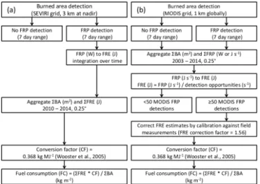
ap-proach, but now including 5 years of SEVIRI data (2010– 2014), to get a better understanding of fuel consumption in infrequently burning zones and to derive more representative mean fuel consumption estimates in general. An overview of this method is given in the flow chart of Fig. 1a and explained in more detail below.
First, the daily burned-area data (500 m resolution) were reprojected to the native SEVIRI imaging grid (3 km reso-lution at nadir). Because of the uncertainty in the burn date in the burned-area product (Boschetti et al., 2010; Giglio et al., 2013), and the fact that a fire can burn for multiple days, we followed Roberts et al. (2011) and assumed that all FRP detections within one week of the burned area observations (before or after; i.e. in total 15 days) in a given grid cell be-longed to the same fire. Roberts et al. (2011) investigated the distribution of active fire detections in the days around the “day of burn” as determined by the burned-area dataset and showed that > 80 % of the SEVIRI active fire detections occurred within 2 days before or after the day of burn, af-ter which the sensitivity rapidly decreases. Use of a 15-day time window thus includes nearly all FRE that can be asso-ciated with a given fire, while the possible effect of small fires with observed FRP but without corresponding burned area (burning within the same pixel and time window) on the fuel consumption estimates is likely small. Grid cells having only burned-area observations but no corresponding FRP de-tections are likely related to fires having relatively low FRP or those that were obscured by clouds (Roberts et al., 2011). These areas (3 % of annual burned area) were excluded from our analysis. Moreover, about half (54 %) of the burned-area detections showed over 20 % cloud cover and/or missing data during the 15-day accumulation period, possibly reducing FRE estimates. We decided not to exclude these data so as to maintain as large a sample as possible, but we investigated the impact of this effect via a comparison of results including and excluding partial cloud cover and missing data.
As a second step, the 15 min interval SEVIRI FRP detec-tions were integrated over time to calculate FRE. This FRE was then converted into dry matter burned using the conver-sion factor (0.368 kg MJ−1)based on lab experiments of var-ious fuel types by Wooster et al. (2005). We limited the study to the spatial distribution of mean fuel consumption and cal-culated fuel consumption (FC) for each 0.25◦grid cell (x, y) based on
FC(SEVIRI)x,y=
P2014
2010DM_burnedx,y
P2014 2010BAx,y
, (1)
whereP20142010DM_burned corresponds to the sum of dry mat-ter burned of each SEVIRI grid cell within the coarser 0.25◦
grid over the study period with a corresponding burned-area observation, andP20142010BA is the sum of burned area (BA) for each 0.25◦ grid cell with corresponding FRE over the study period.
3.2 Converting MODIS FRP to fuel consumption using in situ measurements
With approximately four daily overpasses, MODIS provides only a sample of daily fire activity and FRP. Various ap-proaches have been developed to derive FRE (J) and dry mat-ter burned (kg) estimates from the MODIS FRP data (e.g. El-licott et al., 2009; Freeborn et al., 2009, 2011; Kaiser et al., 2012; Vermote et al., 2009). However, methods to convert MODIS FRP to FRE usually work at the relatively coarse spatial and/or temporal scale (e.g. 0.5◦monthly) required to
accumulate a statistically valid number of FRP observations. The sensitivity of the MODIS burned-area product to “small fires” is considerably worse than that of the MODIS active fire product (Randerson et al., 2012), and within each rela-tively large grid cell the proportion of FRP observations that originate from these small (unmapped) burned areas remains unknown. Therefore, these methods cannot directly be used to estimate fuel consumption. The method developed here to derive FRE is similar to the one used within the GFAS version 1 (Heil et al., 2010; Kaiser et al., 2012), but obser-vations of “small fires” (having FRP detections but no cor-responding burned area) were discarded (by working at the native MODIS 1 km resolution). Because the objective here was to estimate fuel consumption per unit area burned instead of total dry matter burned, the impact of ignoring the small-est fires is small, as long as fuel consumption in such fires is of a similar magnitude or their relative fraction is low. An overview of the method is shown in the flow chart of Fig. 1b, and explained in more detail below.
The FRP recorded by the polar-orbiting MODIS instru-ments are affected by the MODIS scan geometry (Free-born et al., 2011), cloud cover, tree cover (Free(Free-born et al., 2014b), and the fire diurnal cycle and daily number and tim-ing of overpasses (Andela et al., 2015). Hence, whilst a sin-gle MODIS FRP detection is somewhat representative of the overall fire activity in a certain grid cell, its value is also influenced by these other factors (e.g. Andela et al., 2015; Boschetti and Roy, 2009; Freeborn et al., 2009). Moreover, temporal variations in fuel consumption may be consider-able, driven by climate, vegetation type, management, and fire return periods (Hély et al., 2003a; Savadogo et al., 2007; Shea et al., 1996). Minimizing the impact of these types of perturbations is in part why methods developed to es-timate FRE from MODIS FRP generally require the accu-mulation of MODIS FRP observations over relatively coarse spatiotemporal scales (e.g. Freeborn et al., 2009; Vermote et al., 2009). We further investigated the combined effect of all these factors on the FRP data by studying the distribution of FRP observations for a frequently burning grid cell in Africa. Following the methods applied within GFAS (Heil et al., 2010; Kaiser et al., 2012), FRE was estimated by assuming that the observed daily fire activity (i.e. FRP) at cloud-free MODIS overpasses is representative of daily fire activity. To create a sufficiently large and “representative” sample size, burned-area detections and FRP detections with correspond-ing burned area were aggregated to a 0.25◦spatial resolution for the full period that both Aqua and Terra were in orbit (2003–2014). Subsequently the total emitted FRE (J) over the study period was calculated per grid cell as the sum of FRP (W or J s−1)multiplied by the mean duration between two
MODIS detection opportunities (s) during the burning season (calculated using the mean number of cloud-free overpasses per day weighted by monthly burned area). This way we im-plicitly correct for variation in the daily detection opportu-nity caused by cloud cover and/or the MODIS orbits (e.g. Andela et al., 2015; Kaiser et al., 2012). For further analy-sis we only include those 0.25◦grid cells containing at least 50 MODIS FRP detections (together responsible for 96 % of annual burned area).
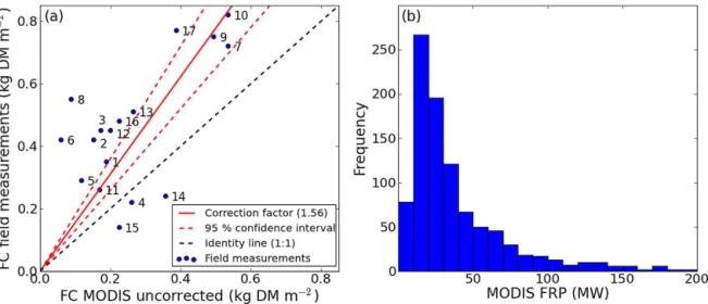
Similar to the method based on the SEVIRI data we used the 0.368 kg MJ−1conversion factor to derive fuel consump-tion (Wooster et al., 2005). However, because of the un-certainties in the FRE estimates, we calibrated our results against field measurements. We used simple linear regression forced through the origin between the uncorrected MODIS-derived fuel consumption (kg m−2)and the corresponding
field measurements of fuel consumption compiled by van Leeuwen et al. (2014) to derive a correction factor between the MODIS-derived FRE per unit area burned (MJ m−2)
and the emitted FRE at the Earth’s surface. Bootstrapping (n=10 000, bias-corrected and accelerated bootstrap) was used to study the uncertainty associated with this correction factor. From the field measurement database we included all measurements conducted in grasslands, savannas and woody
Figure 1. Methods to derive 0.25◦ fuel consumption estimates based on two different approaches.(a)The pathway used to com-bine FRP data of the geostationary SEVIRI instrument with burned-area data to derive fuel consumption (Roberts et al., 2011; Sect. 3.1). (b) The pathway used to derive fuel consumption by combining FRP data of the polar-orbiting MODIS instruments with burned-area data (Sect. 3.2). Note that FRP detections without correspond-ing burned area, associated with small fires, are excluded in both processing chains.
savannas (Table 1). The results were also compared to the results based on the approach using the SEVIRI instrument outlined in Sect. 3.1. However, in that case we did not apply the FRE correction factor so as to better understand the im-pact of the different sensor characteristics and methods used here on the fuel consumption estimates.
4 Results
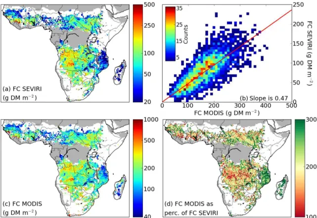
4.1 Comparing SEVIRI- and MODIS-derived fuel consumption
Figure 2.Comparison of fuel consumption (FC) estimates derived by combining FRP and burned-area data.(a)Fuel consumption derived using SEVIRI FRP data.(b)Correlation between fuel consumption estimates based on the SEVIRI and MODIS FRP data.(c)Fuel con-sumption derived using MODIS FRP data.(d)MODIS-based fuel consumption estimates as a percentage of the SEVIRI-based estimates. For comparison both SEVIRI- and MODIS-based estimates are shown for the same period (2010–2014) and the MODIS FRE data are un-corrected (see Sect. 4.2). Note that on average MODIS-derived FC is about twice as large as SEVIRI-derived FC. Grid cells with dominant land cover “forest” or “bare or sparsely vegetated” were excluded from our analysis and are masked grey, while water and grid cells with less than 50 MODIS FRP detections are shown in white in all figures.
(e.g. Mozambique and Madagascar), likely because of the decreasing sensitivity of the SEVIRI instrument at the greater off-nadir angle over this region (e.g. Freeborn et al., 2014b), and second, the relative fraction of FRE emitted during peri-ods that FRP values were below the SEVIRI detection thresh-old, a function of the absolute FRP values and the shape of the fire diurnal cycle. Fires with high FRP (related to high fire spread rates and/or fuel consumption) are often equally well observed by both instruments (i.e. red colouring in Fig. 2d), while areas with low fuel consumption are often character-ized by a larger differences between the MODIS and SE-VIRI estimates (i.e. green colouring in Fig. 2d). To prevent these differences from affecting our estimated correlation too much, we only included frequently burning grid cells (burned area≥15 % yr−1)and those that have a surface area of the SEVIRI FRP-PIXEL product grid cells below 12 km2 (min-imum value is 9 km2 at nadir) during the linear regression shown in Fig. 2b. This resulted in reasonable correlation (r2=0.42;n=6569). Partial cloud cover and missing data were also affecting the analysis, and we found that 54 % of the annual burned area occurred during periods of reduced
data availability (below 80 % during the 15-day time win-dow). When excluding these events, the absolute difference between MODIS- and SEVIRI-based fuel consumption be-came somewhat smaller (i.e. the slope in Fig. 2b bebe-came 0.59), demonstrating that periods of reduced observations were partly responsible for the underestimation in SEVIRI-derived fuel consumption. However, by excluding this 54 % of the data, the correlation between MODIS- and SEVIRI-based fuel consumption was reduced (r2=0.28) due to the heterogeneous nature of fuel consumption.
4.2 Converting MODIS FRP to fuel consumption using in situ measurements
factor ranges from 1.30 to 1.80. In addition the coefficient of determination (r2)between both datasets is considered rea-sonable (0.41), something we return to in the discussion.
Figure 3b shows the distribution of MODIS FRP detec-tions for a frequently burning 0.25◦ grid cell in northern Africa for the 2003–2014 study period. As discussed in the methods, a single MODIS FRP detection is often not rep-resentative of the actual fuel consumption rate or fire activ-ity, and it is more reasonable to take a representative sam-ple (we used a minimum of 50 active fire pixel detections). For this particular 0.25◦grid cell (Fig. 3b), over the full pe-riod there were 967 MODIS FRP detections, having a sum of 39.7 GW, while total burned area was 5.7×10⁹m2. Dur-ing the burnDur-ing season, the two MODIS instruments together observed the grid cell 2.8 times a day on average. The esti-mated FRE per unit area burned was therefore 0.22 MJ m−2.
After applying the correction factor of 1.56 (see Fig. 3a), the estimated FRE per unit area burned becomes 0.34 MJ m−2
and fuel consumption for the grid cell shown in Fig. 3b is 125 g DM m−2. To put this value into context, for this grid cell the mean NPP was 732 g DM m−2yr−1and the mean fire return period 1.75 years over the study period.
Table 1 provides an overview of the field studies used to calibrate the MODIS-based FRE estimates (Fig. 3a), and corresponding 0.25◦ fuel consumption estimates based on MODIS FRP detections. Most fuel consumption estimates based on field measurements are similar in magnitude to the ones derived here, although there are a few prominent out-liers (numbers 6, 8, 14 and 15). The field studies correspond-ing to numbers 15 and 16 were carried out within the same 0.25◦grid cell and illustrate that individual case studies are
not always directly comparable with our 0.25◦fuel
consump-tion estimates due to the large spatial heterogeneity of fuel consumption.
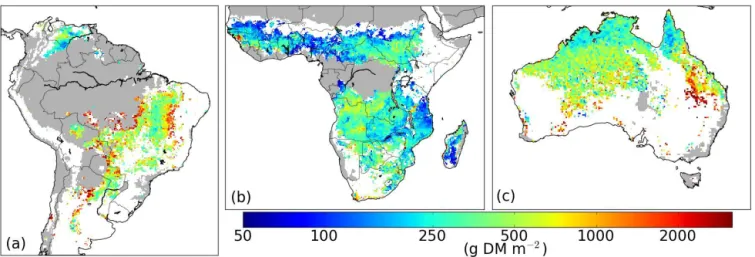
Fuel consumption for the three study regions was de-rived by applying the correction factor (Fig. 3a; 1.56) to the FRE per unit area burned (MJ m−2)as estimated using the MODIS FRP detections over the full period study period (2003–2014; Fig. 4). South America generally showed rel-atively high fuel consumption, with the fringes of the defor-estation areas having by far the highest values (Fig. 4a). Sub-Saharan Africa has relatively low fuel consumption com-pared to Australia and South America, with lowest fuel con-sumption found in eastern Africa and agricultural regions in western Africa (e.g. Nigeria; cf. Figs. 4b and A1h in the Appendix). Australia shows a surprising pattern where fuel consumption according to our approach in frequently burn-ing savannas in northern Australia appears to be lower than fuel consumption in the drier interior (Figs. 4c and A1c). The same pattern is observed in some arid regions of southern Africa where fires have long return periods (e.g. Namibia; Figs. 4b and A1b).
4.3 Drivers and dynamics of fuel consumption
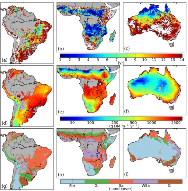
For each continent we assessed whether most fires occurred in productive or low-productivity systems, and whether short or long fire return periods were most common (Fig. 5a–c). Then we explored the distribution of fuel consumption as a function of productivity and fire return periods (Fig. 5d–f), followed by the possible role of land cover type in explaining these patterns (Fig. 5g–i). We found that biomass burning on the three continents occurred under very different conditions in terms of productivity and fire return periods. Within the South American study region most fires occurred in relatively productive savannas (NPP of 800–1600 g DM m−2yr−1)and were characterized by relatively long fire return periods (3– 8 years). Fuel consumption in this region was higher than under similar conditions (in terms of NPP and fire return pe-riod) in Sub-Saharan Africa and Australia. African biomass burning was dominated by (woody) savanna fires of annual and biennial return periods which were observed over a wide range of NPP (500–2000 g DM m−2yr−1). For the lower pro-ductivity African savannas and grasslands, we did not find large differences in fuel consumption between savannas that burn annually or biennially and savannas with somewhat longer return periods (3–8 years). Only African savannas with fire return periods above 8 years showed again a some-what higher fuel consumption. Strikingly, in the more pro-ductive African savannas, fuel consumption declined with longer fire return periods.
In Australia, most burned area occurred in the savan-nas of intermediate-productivity (500–1200 g DM m−2yr−1)
and low-productivity hummock grasslands (< 500 g DM m−2
yr−1; Australian Native Vegetation Assessment, 2001),
which were classified as shrublands by the MODIS land cover dataset. While in Sub-Saharan Africa most fires in the lower productivity regions were fuelled by grasses that form well-connected fuel beds, in Australia most fires occurred in poorly connected hummock grasslands that functionally act like shrublands. Both in Sub-Saharan Africa and in Australia, regions classified as shrubs faced longer fire return peri-ods than grasslands and savannas but eventually burned with higher fuel consumption. But even when productivity and fire return periods were similar the fuel consumption in the low-productivity (< 500 g DM m−2yr−1)hummock grasslands of Australia was consistently higher than fuel consumption of the low-productivity grasslands in Sub-Saharan Africa.
Figure 3.Relationship between MODIS FRP detections and fuel consumption (FC).(a)Comparison of MODIS-derived fuel consumption without correction for uncertainties in the FRE estimates with field measurements of fuel consumption. The slope between the uncorrected MODIS-derived FC and the FC from field measurements (red line; slope is 1.56) is used to correct the MODIS-derived FRE per unit area burned and estimate absolute fuel consumption. The red dashed lines indicate the bootstrapped 95 % confidence interval of the slope (1.30– 1.80), here used as an estimate of uncertainty. The blue dots and numbers refer to the individual field studies (van Leeuwen et al., 2014; Table 1).(b)Distribution of MODIS FRP detections (binned in classes of 10 MW wide) for a frequently burning 0.25◦grid cell in northern Africa (10.00–10.25◦N, 24.00–24.25◦E).
Table 1. Fuel consumption estimates for grasslands, savannas and woody savannas, based on field studies compiled by van Leeuwen et al. (2014) and the corresponding 0.25◦fuel consumption estimates derived here. For the field studies, numbers in parentheses show the standard deviation.Nis the number of active fire detections by MODIS (2003–2014) for each 0.25◦grid cell.
No. Lat Long FC (g DM m−2) FC (g DM m−2) N Description Reference
(Fig. 3a) Field study MODIS
1 25.15◦S 31.14◦E 350 (140) 294 226 Lowveld sour bushveld savanna Shea et al. (1996) and Ward et al. (1996)
2 12.35◦S 30.21◦E 420 (100) 237 1487 Dambo, miombo, chitemene Shea et al. (1996) and Ward et al. (1996) 3 16.60◦S 27.15◦E 450 (–) 269 216 Semi-arid miombo Shea et al. (1996) and Ward et al. (1996)
4 14.52◦S 24.49◦E 220 (120) 405 880 Dambo and miombo Hoffa et al. (1999)
5 15.00◦S 23.00◦E 290 (90) 183 407 Dambo and floodplain Hély et al. (2003b)
6 12.22◦N 2.70◦W 420 (70) 92 177 Grazing and no grazing Savadogo et al. (2007)
7 15.84◦S 47.95◦W 720 (90) 832 126 Different types of cerrado Ward et al. (1992) 8 8.56◦N 67.25◦W 550 (190) 138 232 Protected savanna for 27 years Bilbao and Medina (1996) 9 15.51◦S 47.53◦W 750 (–) 768 69 Campo limpo and campo sujo Miranda et al. (1996) 10 15.84◦S 47.95◦W 820 (280) 832 126 Different types of cerrado De Castro and Kauffman (1998) 11 3.75◦N 60.50◦W 260 (90) 263 35 Different types of cerrado Barbosa and Fearnside (2005)
12 12.40◦S 132.50◦E 450 (130) 311 1885 Woodland Cook et al. (1994)
13 12.30◦S 133.00◦E 510 (–) 413 1277 Tropical savanna Hurst et al. (1994)
14 12.43◦S 131.49◦E 240 (110) 555 433 Grass and woody litter Rossiter-Rachor et al. (2008) 15 12.38◦S 133.55◦E 140 (160) 351 1357 Early and late season fires Russell-Smith et al. (2009) 16 12.38◦S 133.55◦E 480 (–) 351 1357 Grass and open woodland Meyer et al. (2012)
17 17.65◦N 81.75◦E 770 (260) 603 20 Woodland Prasad et al. (2001)
best comparison was found in zones of most frequent fire and short fire return periods (compare Fig. 6 with Fig. A1a–c).
5 Discussion
Understanding the global distribution of fuel consumption per unit area burned, here referred to as fuel consumption for brevity, and fuel build-up mechanisms is important for making landscape management decisions, understanding the
Figure 4.Distribution of fuel consumption based on MODIS-derived FRE per unit of area burned (2003–2014) and calibrated against field studies.(a)South America,(b)Sub-Saharan Africa and(c)Australia.
Figure 5.Distribution of burned area(a–c), fuel consumption(d– f)and dominant land cover type(g–i), all binned as a function of fire return periods and net primary productivity (NPP) for the three study regions (South America, Sub-Saharan Africa and Australia). Bins with burned area below 500 km2yr−1 are masked in white. Abbreviations of land cover type stand for cropland (Cr), woody savanna (WSa), savanna (Sa), grassland (Gr) and shrubland (Sh).
heterogeneous (e.g. Boschetti and Roy, 2009; Hély et al., 2003a; Roberts et al., 2011; Savadogo et al., 2007). Con-sequently, obtaining representative field measurements is labour-intensive, and only a limited number of studies have been carried out (van Leeuwen et al., 2014). Satellite-derived estimates of the spatial distribution of fuel consumption can therefore form an important addition to the scarce field mea-surements and may guide future field campaigns.
Here we discuss the pros and cons of the fuel consumption estimates presented in this paper and the current challenges for such an exercise (Sect. 5.1). We then discuss the drivers of fuel consumption in the three study regions, and compare the results found here to fuel consumption estimates of the GFED4s data (Sect. 5.2).
geosta-tionary data (compare Fig. 2a and c), providing confidence in the spatial distribution of the fuel consumption estimates. However, many differences were also present (Fig. 2d). We found that a large part of the differences could be attributed to the different sensors characteristics and methods used here. The shape of the fire diurnal cycle, for example, affects both MODIS-based fuel consumption estimates due to the lim-ited number of daily overpasses but also the SEVIRI-derived fuel consumption estimates because it directly affects the rel-ative fraction of daily fire activity that falls below the SE-VIRI detection threshold. After excluding grid cells at higher off-nadir angles of the SEVIRI instrument and of infrequent fire occurrence, we found an r2 of 0.42 between both ap-proaches. Finally, a large structural difference was observed, and SEVIRI-derived fuel consumption was about half of the MODIS-derived fuel consumption. Such structural dif-ferences likely occur due to the different sensitivities of the instruments (Freeborn et al., 2009, 2014b). As compared to the MODIS instruments, the SEVIRI instrument likely un-derestimates fire activity in areas where a relatively large fraction of fire activity falls below the detection threshold (e.g. small fires, or fires partly obscured by trees; as discussed by Freeborn et al., 2009, 2014b, Roberts and Wooster, 2008 and Roberts et al., 2011). In our analysis a small part of the structural difference could also be explained by the fact that we did not correct for cloud cover and/or missing data in the SEVIRI-based FC estimates. Not surprisingly, the best com-parison between both methods was found in areas of high fuel consumption rates (Fig. 2d), for example areas where fires can spread over large areas to form large fire fronts (Archibald et al., 2013), and areas of high fuel consumption; these fires with high FRP are likely to be well observed by both instruments.
When deriving fuel consumption estimates based on the SEVIRI instrument, Roberts et al. (2011) found fuel con-sumption estimates around 3.5 times lower than modelled values of GFED3.1 (van der Werf et al., 2010). Other stud-ies that calculated fire emissions using the SEVIRI instru-ment found similar low estimates compared to GFED (e.g. Roberts and Wooster, 2008). Following previous studies, we find that about half of this discrepancy can be attributed to SEVIRI failing to detect the more weakly burning fires that ultimately are responsible for around half of the emitted FRE (Freeborn et al., 2009, 2014b). Similarly, MODIS-derived FRE estimates are also affected by the sensor characteristics and methods used here. We therefore decided to correct for such issues by calibrating the FRE per unit area burned based on the MODIS instruments directly against field observa-tions before converting them to fuel consumption. When us-ing the conversion factor found by Wooster et al. (2005) and the uncorrected MODIS FRE estimates, a slope of 1.56 was found during linear regression between MODIS-derived fuel consumption and fuel consumption estimates based on field measurements (Fig. 3a). Because of the large spatiotemporal variation in fuel consumption and the relatively low sample
size, the 95 % confidence interval of the bootstrapped correc-tion factor was 1.30–1.80. The uncertainty associated with the correction factor is thus around±16 %, although other factors may further affect the uncertainty in our fuel con-sumption estimates as discussed below. The need for a FRE correction factor (1.56) may for a large part be explained by sensor-specific limitations (Giglio et al., 2006a) that likely lead to underestimations of total FRE, particularly due to the reduced sensitivity of the MODIS instruments towards the swath edges (Freeborn et al., 2011). The fire diurnal cycle in combination with the timing of the MODIS overpasses and partial cloud cover may also have affected absolute FRE estimates and thus the FRE correction factor derived here (Andela et al., 2015). Although Freeborn et al. (2011) find a similar correction to be needed due to the decreasing sen-sor sensitivity with increasing scan angle, the number of field measurements was limited and our calibration was strongly influenced by a few field studies in more productive savan-nas. The correlation of the field observations and the 0.25◦ long-term average fuel consumption estimates derived here (Fig. 3a;r2=0.41) was affected by various factors. Most im-portantly, fuel consumption is both spatially and temporarily highly heterogeneous (e.g. Govender et al., 2006; Hély et al., 2003a; Hoffa et al., 1999), so even in the case of accurate fuel consumption estimates from both field measurements and from satellite, large scatter is likely observed. In addition, the fuel consumption estimates derived here are mostly rep-resentative of midday burning during the peak burning sea-son because FRE emitted during these periods will dominate the signal. Finally, direct comparison with the field studies was impossible because most field studies were carried out before the launch of the MODIS and SEVIRI instruments (van Leeuwen et al., 2014).
5.2 Drivers and dynamics of fuel consumption
Fuel consumption depends on the amount of fuel available for burning and the combustion completeness. In arid ar-eas available fuel and thus fuel consumption are often lim-ited by precipitation. Across these arid and semi-arid ar-eas precipitation generally determines vegetation produc-tivity and tree cover. Grasses in these more arid ecosys-tems often have a combustion completeness above 80 % (van Leeuwen et al., 2014), and fuel consumption and fuel loads will generally be similar. In more humid regions, how-ever, fuel moisture may limit fuel consumption by low-ering fire spread and the combustion completeness (Stott, 2000; van der Werf et al., 2008). In our three study regions (South America, Sub-Saharan Africa and Australia) fires oc-curred under very different conditions in terms of NPP and fire return periods (Fig. 5a–c), partially as a result of the different distributions of NPP across the study regions. In South America most burned area occurred in regions with fire return periods between 3 and 8 years and intermedi-ate productivity (800–1600 g DM m−2yr−1). In Africa the vast majority of burned area was found in areas with short fire return periods (1–3 years) and a wide range of pro-ductivity (500–2000 g DM m−2yr−1). In Australia the ma-jority of fires occurred in the more arid low-productivity zones (< 500 g DM m−2yr−1), while annually burning re-gions were uncommon and restricted to the humid higher productivity zones (typical fire return periods were in the range 2 to 10 years). Although climate and vegetation shape the boundary conditions for fires to occur, most ignitions are of human origin (Archibald et al., 2012; Scholes and Archer, 1997; Scholes et al., 2011; Stott, 2000) and the differences between the continents are expected to be partly the result of different management practices. Overall, a pattern of in-creasing fuel consumption towards more productive regions and longer return periods was observed (Fig. 5d–f). Conse-quently, fuel consumption in Africa, with short return pe-riods, was relatively low compared to Australia or South America. However, increases in fuel consumption with in-creasing time between fires and NPP were far from linear and other drivers also played a large role (e.g. Shea et al., 1996).
In more arid regions, we found a clear difference between ecosystems where most fuel exists of grasses opposed to re-gions that were classified as shrubs. In Africa, the rere-gions with NPP below 500 g DM m−2yr−1 are dominated by
sa-vannas or grasslands, while in Australia these regions are classified as shrubs (Fig. 5h and i). In the specific case of Australia, much of the interior is actually dominated by hum-mock grasslands (rather than shrubs), grasses that function-ally act like shrubs (Australian Native Vegetation Assess-ment, 2001) and are therefore classified as being shrublands in the University of Maryland classification. Grasses may form well-connected fuel beds, resulting in short (often an-nual or biennial) fire return periods (Archibald et al., 2013;
Beerling and Osborne, 2006; Scholes and Archer, 1997), while fire return periods in shrublands (or hummock grass-lands) were generally longer (Fig. 5). But on top of the dif-ferences in fire return periods between these low-productivity ecosystems, the grass species that were dominant in most of Africa showed a rather slow fuel build-up compared to shrubs or the Australian hummock grasses even when fire re-turn periods and productivity were similar (Fig. 5e and f). A possible explanation for the relatively slow fuel build-up in African grasslands and savannas as opposed to Australian hummock grasslands and shrublands could be grazing by livestock or wildlife and human management (Savadogo et al., 2007; Scholes et al., 2011). Shea et al. (1996) report a large impact of wildlife, ranging from insects to grazers, on fuel build-up processes in various study sites in Africa, and such effects will differ among continents given that neither South America nor Australia have the diverse and dominant mega-herbivore fauna of Africa. Other differences may come from non-fire-related decomposition rates, which depend on plant species and climate (Gupta and Singh, 1981).
ar-Figure 6. Fuel consumption estimated by GFED4s as a percentage of fuel consumption derived here (based on MODIS-derived FRE, calibrated against in situ measurements).(a)South America,(b)Sub-Saharan Africa and(c)Australia.
eas are experiencing increases in tree cover (Wigley et al., 2010). A clear example was South America, where the appar-ent fuel build-up (Fig. 5d) appears largely driven by high fuel consumption in active deforestation areas (Fig. 4; see Hansen et al., 2013). The effect of human management on fuel loads was also clearly visible in Africa’s agricultural areas (e.g. Nigeria), where fuel loads were typically low (Figs. 4, 5e and h).
Finally, the fuel consumption estimates derived here were compared to the modelled fuel consumption estimates of GFED4s. Within GFED fuel build-up is largely driven by NPP and fire return periods, while biomass build-up is dis-tributed over two different pools: herbaceous and woody (van der Werf et al., 2010). This differentiation is impor-tant, because in savanna ecosystems most fires burn in the grass layer, leaving the older well-established woody vege-tation largely untouched (Scholes and Archer, 1997). Fuel consumption estimates derived here and by GFED were com-parable in annual or biennial burning savannas (Figs. 6 and A1a–c). This is encouraging, because from an emissions per-spective the modelling of fuel consumption has to be most accurate in areas that burn annually or biennially where little long-term fuel build-up takes place. For arid areas in general, but especially for shrublands and the hummock grasslands in Australia, the fuel consumption estimates derived here were considerably larger than the ones estimated by GFED. Part of this difference may be caused by GFED using a universal fuel build-up mechanism for all types of grasses and shrub-lands (van der Werf et al., 2010), which according to our find-ings seems oversimplified. In fact, hummock grasses act like shrubs with bare soil between the mounds of hummock grass (Australian Native Vegetation Assessment, 2001); such be-haviour likely results in very different fuel build-up dynamics which may vary strongly depending on the wet season inten-sity as opposed to other grasses that form a well-connected fuel bed. The enhanced fuel consumption in arid and
semi-arid drylands found here confirms the important role of semi-arid and semi-arid drylands in the inter-annual variability in the global carbon cycle (Poulter et al., 2014).
biogeochemical models, while providing improved insights into the underlying processes.
6 Conclusions
Satellite-derived fuel consumption estimates (with units of kilograms of dry matter per square metre burned) provide a unique opportunity to challenge current understanding of spatiotemporal variation in fuel consumption that to date is mostly based on field studies and modelling. The fuel con-sumption estimates based on fire radiative power (FRP) data of the geostationary SEVIRI and polar-orbiting MODIS in-struments showed good agreement in terms of spatial pat-terns, suggesting that these estimates were generally robust. When converting fire radiative energy (FRE) estimates de-rived from MODIS and SEVIRI to fuel consumption using a conversion factor based on laboratory measurements and mapped burned area, fuel consumption estimates based on MODIS FRP data were about twice as high as the ones based on the SEVIRI data. This can likely be attributed to SE-VIRI failing to detect large parts of the emitted FRE by more weakly burning or (highly numerous) smaller fires, which ul-timately are responsible for around half of the emitted FRE. On top of that, when we calibrated the fuel consumption es-timates based on MODIS FRP detections to field observa-tions, we found that a correction factor of 1.56 was needed for them to match. This discrepancy likely stems from under-estimation of FRE based on the MODIS instruments, for ex-ample related to the decreased sensitivity of the instruments towards the swath edges. Our best estimates of fuel consump-tion based on MODIS-derived FRE using the correcconsump-tion fac-tor based on field observations were similar in magnitude to modelled fuel consumption estimates from GFED4s, but dis-crepancies were found in the spatial patterns. However, the limited number of field studies combined with the high spa-tiotemporal heterogeneity of fuel consumption complicated the comparison of field studies with long-term, coarse-scale satellite-derived products, and uncertainty in absolute esti-mates remained therefore considerable. Field studies espe-cially designed to validate satellite-derived fuel consumption estimates, aiming for example at NPP or fire return period transects, possibly using air-based remote sensing, could im-prove (confidence in) absolute fuel consumption estimates in the future.
Dominant biomass burning conditions in South America, Sub-Saharan Africa and Australia were highly different in terms of NPP and fire return periods, partly driving fuel con-sumption patterns. In South America most fires occurred in savannas with relatively long fire return periods, resulting in relatively high fuel consumption compared to the other study regions. In contrast, most burned area in Sub-Saharan Africa stemmed from (woody) savannas that burned annually or biennial with relatively low fuel consumption. Australian biomass burning was dominated by relatively unproductive (hummock) grasslands with a wide range of fire return peri-ods, while savannas with fire return periods of 2–3 years also contributed.
Besides NPP and fire return periods, vegetation type played an important role in determining the fuel build-up mechanism. Grasslands favoured short fire return peri-ods and were generally characterized by low fuel build-up rates. Shrublands, or grassy species that functionally act like shrubs, on the other hand, were generally character-ized by longer return periods, but gradual fuel build-up oc-curred over the years eventually leading to higher fuel con-sumption. Similarly, land management had a marked effect on fuel consumption. In the major deforestation regions of South America, fires consumed woody biomass during the MODIS era, increasing fuel consumption estimates. Western African fuel consumption was clearly suppressed in some ar-eas, likely associated with agriculture and/or grazing. These results demonstrate that the modelling of fuel consumption is complex, while the relation between climate, vegetation and fuel consumption may vary across the continents depending on, for example, the presence of certain species. During fu-ture investigations, satellite-derived fuel consumption esti-mates may be used as a reference dataset for biochemical models and may help to better understand the interaction be-tween climate, vegetation patterns, landscape management and fuel consumption.
7 Data availability
Appendix A
Acknowledgements. The authors would like to thank the two reviewers for their constructive remarks and the data providing agencies (NASA and EUMETSAT LSA SAF) for making their data publicly available. This study was funded by the EU in the FP7 and H2020 projects MACC-II and MACC-III (contract nos. 283576 and 633080) and the European Research Council (ERC), grant number 280061.
Edited by: K. Thonicke
References
Andela, N. and van der Werf, G. R.: Recent trends in African fires driven by cropland expansion and El Niño to La Niña transition, Nature Climate Change, 4, 791–795, 2014.
Andela, N., Kaiser, J. W., van der Werf, G. R., and Wooster, M. J.: New fire diurnal cycle characterizations to improve fire ra-diative energy assessments made from MODIS observations, At-mos. Chem. Phys., 15, 8831–8846, doi:10.5194/acp-15-8831-2015, 2015.
Andreae, M. and Merlet, P.: Emission of trace gases and aerosols from biomass burning, Global Biogeochem. Cy., 15, 955–966, 2001.
Aouizerats, B., van der Werf, G. R., Balasubramanian, R., and Betha, R.: Importance of transboundary transport of biomass burning emissions to regional air quality in Southeast Asia during a high fire event, Atmos. Chem. Phys., 15, 363–373, doi:10.5194/acp-15-363-2015, 2015.
Archibald, S., Roy, D. P., van Wilgen, B. W., and Scholes, R. J.: What limits fire? An examination of drivers of burnt area in Southern Africa, Glob. Change Biol., 15, 613–630, 2009. Archibald, S., Scholes, R. J., Roy, D. P., Roberts, G., and Boschetti,
L.: Southern African fire regimes as revealed by remote sensing, Int. J. Wildland Fire, 19, 861–878, 2010.
Archibald, S., Staver, A. C., and Levin, S. A.: Evolution of human-driven fire regimes in Africa, P. Natl. Acad. Sci. USA, 109, 847– 852, 2012.
Archibald, S., Lehmann, C. E. R., Gómez-Dans, J. L., and Brad-stock, R. A.: Defining pyromes and global syndromes of fire regimes, P. Natl. Acad. Sci. USA, 110, 6442–6447, 2013. Australian Native Vegetation Assessment: National Land and Water
Resources Audit, Canberra, Australia, 2001.
Barbosa, R. I. and Fearnside, P. M.: Above-ground biomass and the fate of carbon after burning in the savannas of Roraima, Brazilian Amazonia, Forest Ecol. Manag., 216, 295–316, 2005.
Beerling, D. J. and Osborne, C. P.: The origin of the savanna biome, Glob. Change Biol., 12, 2023–2031, 2006.
Bilbao, B. and Medina, E.: Types of grassland fires and nitro-gen volatilization in tropical savannas of Venezuela, in: Biomass burning and global change: Biomass burning in South America, Southeast Asia, and temperate and boreal ecosystems and the oil fires of Kuwait, edited by: Levine, J. S., 1996.
Bond, W. J.: What Limits Trees in C4Grasslands and Savannas?, Annu. Rev. Ecol. Evol. S., 39, 641–659, 2008.
Bond, W. J., Woodward, F. I., and Midgley, G. F.: The global distri-bution of ecosystems in a world without fire, New Phytol., 165, 525–537, 2005.
Boschetti, L. and Roy, D. P.: Strategies for the fusion of satel-lite fire radiative power with burned area data for fire ra-diative energy derivation, J. Geophys. Res., 114, D20302, doi:10.1029/2008JD011645, 2009.
Boschetti, L., Roy, D. P., Justice, C. O., and Giglio, L.: Global as-sessment of the temporal reporting accuracy and precision of the MODIS burned area product, Int. J. Wildland Fire, 19, 705–709, 2010.
Bowman, D. M. J. S., Balch, J. K., Artaxo, P., Bond, W. J., Carlson, J. M., Cochrane, M. A., D’Antonio, C. M., Defries, R. S., Doyle, J. C., Harrison, S. P., Johnston, F. H., Keeley, J. E., Krawchuk, M. A., Kull, C. A., Marston, J. B., Moritz, M. A., Prentice, I. C., Roos, C. I., Scott, A. C., Swetnam, T. W., van der Werf, G. R., and Pyne, S. J.: Fire in the Earth system, Science, 324, 481–484, 2009.
Chen, Y., Morton, D. C., Jin, Y., Gollatz, G. J., Kasibhatla, P. S., van der Werf, G. R., Defries, R. S., and Randerson, J. T.: Long-term trends and interannual variability of forest, savanna and agricul-tural fires in South America, Carbon Manag., 4, 617–638, 2013. Cook, G. D.: The fate of nutrients during fires in a tropical savanna,
Aust. J. Ecol., 19, 359–365, 1994.
Crutzen, P. J., Heidt, L. E., Krasnec, J. P., Pollock, W. H., and Seiler, W.: Biomass burning as a source of atmospheric gases CO, H2, N2O, NO, CH3Cl and COS, Nature, 282, 253–256, 1979. De Castro, E. A. and Kauffman, J. B.: Ecosystem structure in
the Brazilian Cerrado: a vegetation gradient of aboveground biomass, root mass and consumption by fire, J. Trop. Ecol., 14, 263–283, 1998.
Ellicott, E., Vermote, E., Giglio, L., and Roberts, G.: Estimating biomass consumed from fire using MODIS FRE, Geophys. Res. Lett., 36, L13401, doi:10.1029/2009GL038581, 2009.
Freeborn, P. H., Wooster, M. J., Roberts, G., Malamud, B. D., and Xu, W.: Development of a virtual active fire product for Africa through a synthesis of geostationary and polar orbiting satellite data, Remote Sens. Environ., 113, 1700–1711, 2009.
Freeborn, P. H., Wooster, M. J., and Roberts, G.: Addressing the spatiotemporal sampling design of MODIS to provide estimates of the fire radiative energy emitted from Africa, Remote Sens. Environ., 115, 475–489, 2011.
Freeborn, P. H., Cochrane, M. A., and Wooster, M. J.: A Decade Long, Multi-Scale Map Comparison of Fire Regime Parame-ters Derived from Three Publically Available Satellite-Based Fire Products: A Case Study in the Central African Republic, Remote Sens., 6, 4061–4089, 2014a.
Freeborn, P. H., Wooster, M. J., Roberts, G., and Xu, W.: Evalu-ating the SEVIRI Fire Thermal Anomaly Detection Algorithm across the Central African Republic Using the MODIS Active Fire Product, Remote Sens., 6, 1890–1917, 2014b.
Friedl, M. A., McIver, D. K., Hodges, J. C. F., Zhang, X. Y., Mu-choney, D., Strahler, A. H., Woodcock, C. E., Gopal, S., Schnei-der, A., Cooper, A., Baccini, A., Gao, F., and Schaaf, C.: Global land cover mapping from MODIS: algorithms and early results, Remote Sens. Environ., 83, 287–302, 2002. (data available at: http://reverb.echo.nasa.gov)
doi:10.1029/2005JG000142, 2006a. (data available at: http:// reverb.echo.nasa.gov)
Giglio, L., van der Werf, G. R., Randerson, J. T., Collatz, G. J., and Kasibhatla, P.: Global estimation of burned area using MODIS active fire observations, Atmos. Chem. Phys., 6, 957– 974, doi:10.5194/acp-6-957-2006, 2006b.
Giglio, L., Loboda, T., Roy, D. P., Quayle, B., and Justice, C. O.: An active-fire based burned area mapping algorithm for the MODIS sensor, Remote Sens. Environ., 113, 408–420, 2009. (data avail-able at: http://modis-fire.umd.edu)
Giglio, L., Randerson, J. T., and van der Werf, G. R.: Analy-sis of daily, monthly, and annual burned area using the fourth-generation global fire emissions database (GFED4), J. Geophys. Res.-Biogeo., 118, 317–328, doi:10.1002/jgrg.20042, 2013. Govender, N., Trollope, W. S. W., and van Wilgen, B. W.: The effect
of fire season, fire frequency, rainfall and management on fire intensity in savanna vegetation in South Africa, J. Appl. Ecol., 43, 748–758, 2006.
Grégoire, J. M., Eva, H. D., Belward, A. S., Palumbo, I., Simonetti, D., and Brink, A.: Effect of land-cover change on Africa’s burnt area, Int. J. Wildland Fire, 22, 107–120, 2013.
Gupta, S. R. and Singh, J. S.: The effect of plant species, weather variables and chemical composition of plant material on decom-position in a tropical grassland, Plant Soil, 59, 99–117, 1981. Hansen, M. C., Potapov, P. V., Moore, R., Hancher, M., Turubanova,
S. A., Tyukavina, A., Thau, D., Stehman, S. V., Goetz, S. J., Loveland, T. R., Kommareddy, A., Egorov, A., Chini, L., Justice, C. O., and Townshend, J. R. G.: High-resolution global maps of 21st-century forest cover change, Science, 342, 850–853, 2013. Heil, A., Kaiser, J. W., van der Werf, G. R., Wooster, M. J., Schultz,
M. G., and van der Gon, H. D.: Assessment of the Real-Time Fire Emissions (GFASv0) by MACC, Tech. Memo. 628, ECMWF, Reading, UK, 2010.
Hély, C., Dowty, P. R., Alleaume, K. K., Korontzi, S., Swap, R. J., Shugart, H. H., and Justice, C. O.: Regional fuel load for two cli-matically contrasting years in southern Africa, J. Geophys. Res., 108, 8475, doi:10.1029/2002JD002341, 2003a.
Hély, C., Alleaume, S., Swap, R. J., Shugart, H. H., and Justice, C. O.: SAFARI-2000 characterization of fuels, fire behavior, com-bustion completeness, and emissions from experimental burns in infertile grass savannas in western Zambia, J. Arid Environ., 54, 381–394, 2003b.
Hoffa, E. A., Ward, D. E., Hao, W. M., Susott, R. A., and Waki-moto, R. H.: Seasonality of carbon emissions from biomass burn-ing in a Zambian savanna, J. Geophys. Res., 104, 13841–13853, doi:10.1029/1999JD900091, 1999.
Hurst, D. F., Griffith, D. W. T., Carras, J. N., Williams, D. J., and Fraser, P. J.: Measurements of trace gases emitted by Australian savanna fires during the 1990 dry season, J. Atmos. Chem., 18, 33–56, 1994.
Kaiser, J. W., Heil, A., Andreae, M. O., Benedetti, A., Chubarova, N., Jones, L., Morcrette, J.-J., Razinger, M., Schultz, M. G., Suttie, M., and van der Werf, G. R.: Biomass burning emis-sions estimated with a global fire assimilation system based on observed fire radiative power, Biogeosciences, 9, 527–554, doi:10.5194/bg-9-527-2012, 2012.
Langenfelds, R. L., Francey, R. J., Pak, B. C., Steele, L. P., Lloyd, J., Trudinger, C. M., and Allison, C. E.: Interannual growth rate varations of atmpospheric CO2and its13C, H2, CH4 and CO
between 1992 and 1999 linked to biomass burning, Global Bio-geochem. Cy., 16, 1048, doi:10.1029/2001GB001466, 2002. Langmann, B., Duncan, B., Textor, C., Trentmann, J., and van der
Werf, G. R.: Vegetation fire emissions and their impact on air pollution and climate, Atmos. Environ., 43, 107–116, 2009. Lehmann, C. E. R., Archibald, S. A., Hoffmann, W. A., and Bond,
W. J.: Deciphering the distribution of the savanna biome., New Phytol., 191, 197–209, 2011.
Lehmann, C. E. R., Anderson, T. M., Sankaran, M., Higgins, S. I., Archibald, S., Hoffmann, W. A., Hanan, N. P., Williams, R. J., Fensham, R. J., Felfili, J., Hutley, L. B., Ratnam, J., San Jose, J., Montes, R., Franklin, D., Russell-Smith, J., Ryan, C. M., Duri-gan, G., Hiernaux, P., Haidar, R., Bowman, D. M. J. S., and Bond, W. J.: Savanna vegetation-fire-climate relationships differ among continents, Science, 343, 548–552, 2014.
Le Page, Y., Oom, D., Silva, J. M. N., Jönsson, P., and Pereira, J. M. C.: Seasonality of vegetation fires as modified by human action: observing the deviation from eco-climatic fire regimes, Global Ecol. Biogeogr., 19, 575–588, 2010.
Meyer, C. P., Cook, G. D., Reisen, F., Smith, T. E. L., Tattaris, M., Russell-Smith, J., Maier, S. W., Yates, C. P., and Wooster, M. J.: Direct measurements of the seasonality of emission fac-tors from savanna fires in northern Australia, J. Geophys. Res.-Atmos., 117, D20305, doi:10.1029/2012JD017671, 2012. Miranda, H. S., Rocha e Silva, E. P., and Miranda, A. C.:
Compor-tamento do fogo em queimadas de campo sujo, in: Impactos de Queimadas em Areas de Cerrado e Restinga, edited by: Miranda, H. S., Saito, C. H., and Dias, B. F. S., Universidade de Brasilia, Brasilia, DF, Brazil, 1–10, 1996.
Moncrieff, G. R., Lehmann, C. E. R., Schnitzler, J., Gambiza, J., Hiernaux, P., Ryan, C. M., Shackleton, C. M., Williams, R. J., and Higgins, S. I.: Contrasting architecture of key African and Australian savanna tree taxa drives intercontinental structural di-vergence, Global Ecol. Biogeogr., 23, 1235–1244, 2014. Padilla, M., Stehman, S. V., Litago, J., and Chuvieco, E.: Assessing
the temporal stability of the accuracy of a time series of burned area products, Remote Sens., 6, 2050–2068, 2014.
Poulter, B., Frank, D., Ciais, P., Myneni, R. B., Andela, N., Bi, J., Broquet, G., Canadell, J. G., Chevallier, F., Liu, Y. Y., Running, S. W., Sitch, S., and van der Werf, G. R.: Contribution of semi-arid ecosystems to interannual variability of the global carbon cycle, Nature, 509, 600–603, 2014.
Prasad, V. K., Kant, Y., Gupta, P. K., Sharma, C., Mitra, A. P., and Badarinath, K. V. S.: Biomass and combustion characteristics of secondary mixed deciduous forests in Eastern Ghats of India, At-mos. Environ., 35, 3085–3095, 2001.
Randerson, J. T., Chen, Y., van der Werf, G. R., Rogers, B. M., and Morton, D. C.: Global burned area and biomass burning emissions from small fires, J. Geophys. Res., 117, G04012, doi:10.1029/2012JG002128, 2012.
Roberts, G., Wooster, M. J., Perry, G. L. W., Drake, N., Rebelo, L.-M., and Dipotso, F.: Retrieval of biomass combustion rates and totals from fire radiative power observations: Application to southern Africa using geostationary SEVIRI imagery, J. Geo-phys. Res., 110, D21111, doi:10.1029/2005JD006018, 2005. Roberts, G., Wooster, M. J., and Lagoudakis, E.: Annual and diurnal
Roberts, G., Wooster, M. J., Freeborn, P. H., and Xu, W.: Integration of geostationary FRP and polar-orbiter burned area datasets for an enhanced biomass burning inventory, Remote Sens. Environ., 115, 2047–2061, 2011.
Roberts, G. J. and Wooster, M. J.: Fire Detection and Fire Charac-terization Over Africa Using Meteosat SEVIRI, IEEE T. Geosci. Remote, 46, 1200–1218, 2008.
Rossiter-Rachor, N. A., Setterfield, S. A., Douglas, M. M., Hutley, L. B., and Cook, G. D.: Andropogon gayanus (gamba grass) in-vasion increases fire-mediated nitrogen losses in the tropical sa-vannas of northern Australia, Ecosystems, 11, 77–88, 2008. Roy, D. P. and Boschetti, L.: Southern Africa Validation of the
MODIS, L3JRC, and GlobCarbon Burned-Area Products, IEEE T. Geosci. Remote, 47, 1032–1044, 2009.
Roy, D. P., Boschetti, L., Justice, C. O., and Ju, J.: The collection 5 MODIS burned area product – Global evaluation by comparison with the MODIS active fire product, Remote Sens. Environ., 112, 3690–3707, 2008.
Running, S. W., Nemani, R. R., Heinsch, F. A., Zhao, M., Reeves, M., and Hashimoto, H.: A Continuous Satellite-Derived Measure of Global Terrestrial Primary Production, Bioscience, 54, 547– 560, 2004. (data available at: http://reverb.echo.nasa.gov) Russell-Smith, J., Murphy, B. P., Meyer, C. P., Cook, G. D., Maier,
S., Edwards, A. C., Schatz, J., and Brocklehurst, P.: Improving estimates of savanna burning emissions for greenhouse account-ing in northern Australia: Limitations, challenges, applications, Int. J. Wildland Fire, 18, 1–18, 2009.
Sankaran, M., Hanan, N. P., Scholes, R. J., Ratnam, J., Augustine, D. J., Cade, B. S., Gignoux, J., Higgins, S. I., Le Roux, X., Lud-wig, F., Ardo, J., Banyikwa, F., Bronn, A., Bucini, G., Caylor, K. K., Coughenour, M. B., Diouf, A., Ekaya, W., Feral, C. J., Febru-ary, E. C., Frost, P. G. H., Hiernaux, P., Hrabar, H., Metzger, K. L., Prins, H. H. T., Ringrose, S., Sea, W., Tews, J., Worden, J., and Zambatis, N.: Determinants of woody cover in African sa-vannas, Nature, 438, 846–849, 2005.
Sankaran, M., Ratnam, J., and Hanan, N.: Woody cover in African savannas: The role of resources, fire and herbivory, Global Ecol. Biogeogr., 17, 236–245, 2008.
Savadogo, P., Zida, D., Sawadogo, L., Tiveau, D., Tigabu, M., and Odén, P. C.: Fuel and fire characteristics in savanna-woodland of West Africa in relation to grazing and dominant grass type, Int. J. Wildland Fire, 16, 531–539, 2007.
Scholes, R. J. and Archer, S. R.: Tree-grass interactions in savannas, Annu. Rev. Ecol. Syst., 28, 517–544, 1997.
Scholes, R. J., Archibald, S., and von Maltitz, G.: Emissions from Fire in Sub-Saharan Africa: the Magnintude of Sources, Their Variability and Uncertainty, Glob. Environ. Res., 15, 53–63, 2011.
Shea, R. W., Shea, B. W., Kauffman, J. B., Ward, D. E., Hask-ins, C. I., and Scholes, M. C.: Fuel biomass and combus-tion factors associated with fires in savanna ecosystems of South Africa and Zambia, J. Geophys. Res., 101, 23551–23568, doi:10.1029/95JD02047, 1996.
Staver, A. C., Archibald, S., and Levin, S. A.: The Global Extent and Determinants of Savanna and Forest as Alternative Biome States, Science, 334, 230–232, 2011.
Stott, P.: Combustion in tropical biomass fires: a critical review, Prog. Phys. Geog., 24, 355–377, 2000.
Turquety, S., Hurtmans, D., Hadji-Lazaro, J., Coheur, P.-F., Cler-baux, C., Josset, D., and Tsamalis, C.: Tracking the emission and transport of pollution from wildfires using the IASI CO re-trievals: analysis of the summer 2007 Greek fires, Atmos. Chem. Phys., 9, 4897–4913, doi:10.5194/acp-9-4897-2009, 2009. van der Werf, G. R., Randerson, J. T., Giglio, L., Gobron, N., and
Dolman, A. J.: Climate controls on the variability of fires in the tropics and subtropics, Global Biogeochem. Cy., 22, GB3028, doi:10.1029/2007GB003122, 2008.
van der Werf, G. R., Randerson, J. T., Giglio, L., Collatz, G. J., Mu, M., Kasibhatla, P. S., Morton, D. C., DeFries, R. S., Jin, Y., and van Leeuwen, T. T.: Global fire emissions and the contribution of deforestation, savanna, forest, agricultural, and peat fires (1997–2009), Atmos. Chem. Phys., 10, 11707–11735, doi:10.5194/acp-10-11707-2010, 2010. (data available at: http: //globalfiredata.org)
van Leeuwen, T. T., van der Werf, G. R., Hoffmann, A. A., Detmers, R. G., Rücker, G., French, N. H. F., Archibald, S., Carvalho Jr., J. A., Cook, G. D., de Groot, W. J., Hély, C., Kasischke, E. S., Kloster, S., McCarty, J. L., Pettinari, M. L., Savadogo, P., Al-varado, E. C., Boschetti, L., Manuri, S., Meyer, C. P., Siegert, F., Trollope, L. A., and Trollope, W. S. W.: Biomass burning fuel consumption rates: a field measurement database, Biogeo-sciences, 11, 7305–7329, doi:10.5194/bg-11-7305-2014, 2014. Vermote, E., Ellicott, E., Dubovik, O., Lapyonok, T., Chin, M.,
Giglio, L., and Roberts, G. J.: An approach to estimate global biomass burning emissions of organic and black carbon from MODIS fire radiative power, J. Geophys. Res., 114, D18205, doi:10.1029/2008JD011188, 2009.
Ward, D. E., Susott, R. A., Kauffman, J. B., Babbitt, R. E., Cummings, D. L., Dias, B., Holben, B. N., Kaufman, Y. J., Rasmussen, R. A., and Setzer, A. W.: Smoke and fire characteristics for cerrado and deforestation burns in Brazil: BASE-B experiment, J. Geophys. Res., 97, 14601–14619, doi:10.1029/92JD01218, 1992.
Ward, D. E., Hao, W. M., Susott, R. A., Babbitt, R. E., Shea, R. W., Kauffman, J. B., and Justice, C. O.: Effect of fuel composition on combustion efficiency and emission factors for African savanna ecosystems, J. Geophys. Res., 101, 23569– 23576, doi:10.1029/95JD02595, 1996.
Wigley, B. J., Bond, W. J., and Hoffman, M. T.: Thicket expansion in a South African savanna under divergent land use: Local vs. global drivers?, Glob. Change Biol., 16, 964–976, 2010. Wooster, M., Roberts, G., Perry, G. L. W., and Kaufman, Y.:
Re-trieval of biomass combustion rates and totals from fire radiative power observations: FRP derivation and calibration relationships between biomass consumption, J. Geophys. Res., 110, D24311, doi:10.1029/2005JD006318, 2005.