www.atmos-chem-phys.net/10/12173/2010/ doi:10.5194/acp-10-12173-2010
© Author(s) 2010. CC Attribution 3.0 License.
Chemistry
and Physics
Comparison of global inventories of CO emissions from biomass
burning derived from remotely sensed data
D. Stroppiana1, P. A. Brivio1, J.-M. Gr´egoire2, C. Liousse3, B. Guillaume3, C. Granier4,5,6, A. Mieville4, M. Chin5, and G. P´etron6,7
1CNR-IREA, Consiglio Nazionale delle Ricerche – Istituto per il Rilevamento Elettromagnetico dell’Ambiente, Milano, Italy 2Joint Research Centre (JRC) of the European Commission, Institute for Environment and Sustainability (IES), Global Environment Monitoring Unit (GEM), Ispra (VA), Italy
3Laboratoire d’A´erologie, UMR 5560, Toulouse, France 4Service d’A´eronomie/CNRS, Paris, France
5NASA/Goddard Space Flight Center, Greenbelt, MD, USA
6NOAA Global Monitoring Division, Earth System Research Laboratory, Boulder, CO, USA
7University of Colorado, Cooperative Institute for Research in Environmental Sciences, Boulder, CO, USA Received: 6 July 2010 – Published in Atmos. Chem. Phys. Discuss.: 22 July 2010
Revised: 30 November 2010 – Accepted: 12 December 2010 – Published: 22 December 2010
Abstract. We compare five global inventories of monthly CO emissions named VGT, ATSR, MODIS, GFED3 and MOPITT based on remotely sensed active fires and/or burned area products for the year 2003. The objective is to highlight similarities and differences by focusing on the geographi-cal and temporal distribution and on the emissions for three broad land cover classes (forest, savanna/grassland and agri-culture). Globally, CO emissions for the year 2003 range be-tween 365 Tg CO (GFED3) and 1422 Tg CO (VGT). Despite the large uncertainty in the total amounts, some common spa-tial patterns typical of biomass burning can be identified in the boreal forests of Siberia, in agricultural areas of East-ern Europe and Russia and in savanna ecosystems of South America, Africa and Australia. Regionally, the largest differ-ence in terms of total amounts (CV>100%) and seasonality is observed at the northernmost latitudes, especially in North America and Siberia where VGT appears to overestimate the area affected by fires. On the contrary, Africa shows the best agreement both in terms of total annual amounts (CV=31%)
and of seasonality despite some overestimation of emissions from forest and agriculture observed in the MODIS inven-tory. In Africa VGT provides the most reliable seasonality. Looking at the broad land cover types, the range of contribu-tion to the global emissions of CO is 64–74%, 23–32% and 3–4% for forest, savanna/grassland and agriculture,
respec-Correspondence to: D. Stroppiana ([email protected])
tively. These results suggest that there is still large uncer-tainty in global estimates of emissions and it increases if the comparison is carried by out taking into account the temporal (month) and spatial (0.5◦×0.5◦ cell) dimensions. Besides
the area affected by fires, also vegetation characteristics and conditions at the time of burning should also be accurately parameterized since they can greatly influence the global es-timates of CO emissions.
1 Introduction
increased fires in the boreal regions and in the tropics and to a strong atmospheric CO anomaly (Langenfelds et al., 2002; Novelli et al., 2003; van der Werf et al., 2004). Moreover, CO is an important sink for hydroxyl radicals (OH) and it is a precursor of ozone (O3)and for these reasons it plays a key role in chemical transport models of atmospheric pollutants (Jain, 2007).
The remaining fraction of total carbon emitted by fires (5%) is released as particulate matter (Reid et al., 2005). Even if lower in percent, these particles have a strong ef-fect on the radiation budget. The aerosols released by the combustion process scatter and absorb incoming solar radi-ation and change the atmospheric radiradi-ation budget (Hobbs et al., 1997; Podgorny et al., 2003) besides their influence on cloud formation and on cloud microphysical processes (Langmann et al., 2009). Black carbon, which constitutes 5–10% of the particle emissions from fires (Liousse et al., 1996; Reid et al., 2005) and has a direct effect on absorbing radiation in the atmosphere, can also reduce albedo when de-posited on snow and ice, thus inducing a positive radiative forcing (global warming). Also, land cover change, which is one of the main causes of vegetation fires, itself induces a change of surface albedo.
These are only some of the major and complex processes that impact on the global climate and have been discussed in a number of studies (Innes et al., 2000). Also, climate vari-ability and change itself can influence fire frequency (Wester-ling et al., 2006). Finally, let us note that recent publications have pointed out that fires can be a source of extremely toxic products such as mercury (Friedli et al., 2009).
Great uncertainty still exists in the assessment of gas and particulate emissions because of the higher temporal dy-namic of vegetation fires with respect to other sources such as fossil fuel combustion (Liousse et al., 2004; Langmann et al., 2009); fires vary from place to place and from year to year and are characterized by high seasonality (Anyamba et al., 2003; H´ely et al., 2003; Boschetti et al., 2004; Michel et al., 2005). Remotely sensed data potentially have all the characteristics for quantifying seasonal and inter-annual in-formation on the emissions from vegetation fires because of their global and quasi continuous coverage (Cooke et al., 1996; Generoso et al., 2003). Moreover, the high frequency of acquisition of satellite data is particularly suited for com-pounds such as CO since its average global lifetime in the atmosphere is about two months.
Two approaches have so far been developed to estimate CO emissions from fires. The bottom-up approach relies on the model provided by Seiler and Crutzen (1980) and has been widely applied at continental and global scales with var-ious spaceborne sensors (Barbosa et al., 1999; Stroppiana et al., 2000; Conard et al., 2002; Schultz, 2002; Michel et al., 2005; van der Werf et al., 2006; Yan et al., 2006; Konare et al., 2008, Liousse et al., 2010). In this approach, estimates of the surface burned by fires is converted into emitted gases and aerosols with a multiplicative model of parameters which
take into account the amount of biomass available for burn-ing, the biomass actually burned by the fire and the amount of gases and aerosols emitted for each unit of burned biomass. These parameters are generally land cover type dependent.
From the late Nineties, inversion models have been de-veloped to derive emissions from CO concentrations mea-sured in the atmosphere (Manning et al., 1997; Bergam-aschi et al., 2000; P´etron et al., 2002). Exploitation of re-motely sensed concentrations of atmospheric gases is more recent and has rapidly increased with the use of the NASA-MOPITT (Measurements OF Pollution In The Troposphere) instrument (Chevallier et al., 2009; P´etron et al., 2004; Liu et al., 2005; Arellano et al., 2006). The latter is also known as top-down approach and consists of estimating carbon surface fluxes from the atmospheric concentrations.
Large differences in both the geographic distribution and temporal dynamics of global and regional CO emission esti-mates are reported in literature; these differences are primar-ily due to uncertainties in the input data on burned area and fuel loads (Langmann et al., 2009) and in either modeling or inversion techniques (P´etron et al., 2004).
Recent developments in remote sensing have made widely available global datasets of active fires and burned areas, which can be exploited for the estimation of emission. Ac-tive fire counts (the number of acAc-tive fires per grid cell) have been used for a long time for depicting temporal and spatial patterns of vegetation fires (Cooke et al., 1996; Dwyer et al., 2000) as well as for quantifying the area burned (Giglio et al., 2006). Since active fire mapping relies on the detection of the high thermal emission from the flaming front of the fire, it is an important source of information for the detection of small events and of fires burning below dense canopies. However, active fire mapping is significantly affected by the presence of clouds at the time of observation and is a sample of the total daily fire activity. By integrating the perimeter of the area affected by the fire, a burned area product should provide a better quantification of the area affected by the fire. Burned area mapping is less affected by could cover due to the persistence of the burned signal. However, burned area mapping can be rather difficult over large areas especially where the remotely sensed signal can be confused with other surface targets (e.g. low albedo surfaces such as shadows, water and some types of soil). Since neither active fire counts nor burned area mapping can provide a satisfying global pic-ture of the geographical and temporal variability of vegeta-tion fires, both are still used by the scientific community for the estimation of the emission.
savanna/grassland and agriculture. The comparison of global inventories of CO emissions from biomass burning is of par-ticular interest for the atmospheric science community since emissions from fires are the least known input to models of atmospheric circulation (Bian et al., 2007).
Despite the large literature on regional estimates, very few studies have attempted so far to compare global datasets of burned areas or pyrogenic emissions from fires and even fewer have specifically addressed the issue of comparing both spatial and temporal distributions (Bian et al., 2007; Jain, 2007; Chang and Song, 2009). The inventories anal-ysed here are derived from different burned area and/or ac-tive fire products and satellite sensors; four of them are based on a bottom-up approach while a fifth dataset is derived with a top-down approach which exploits the concentrations of at-mospheric gases as measured by the MOPITT instrument and inverse modelling techniques. We also analyze the distribu-tion of CO sources among forest, savanna/grassland and agri-culture land cover classes for the VGT, ATSR and MODIS products. We focused on CO emissions because biomass burning is the major source of this chemical compound in the troposphere. Moreover, CO emissions are often used as a reference for the estimation of other pollutants during the combustion process (Andreae and Merlet, 2001).
2 Data and methods
The five CO inventories (Table 1) can be divided into three categories. In the first category, three inventories (VGT, ATSR and MODIS) were built directly from recent global fire products derived from satellite time series which were processed to map either the occurrence of fire events or the area burned. These inventories used common land cover map and set of biomass densities, burning efficiency coefficients and emission factors. The common land cover map selected for this work is the Global Land Cover 2000 (GLC2000) (Bartholom´e and Belward, 2005) built from the 1 km SPOT VEGETATION imagery. The GLC2000 has a spatial reso-lution comparable to those of the remotely sensed fire infor-mation used to build the inventories analysed in this study. Although other land cover maps are available with a finer resolution (e.g. Globcover) we deemed this spatial detail un-suitable for our purposes.
The fourth inventory (GFED3) was also derived from a satellite fire product but with a different set of data for the fuel load, burning efficiency and emission factors. The fifth inventory (MOPITT) was derived from remotely sensed CO observations coupled with an active fire dataset.
2.1 Global CO inventories
2.1.1 The VGT inventory
This inventory was built by the Centre National de la Recherche Scientifique-Laboratoire d’A´erologie
(CNRS-LA) to derive gaseous and particulate emissions for the 2000–2007 period (Liousse et al., 2010). It is based on the L3JRC burned area product (Tansey et al., 2008) derived from the 1 km daily images of the VEGETATION (VGT) sensor onboard the SPOT (Satellite Pour l’Observation de la Terre) satellites. Developed by a consortium of four Eu-ropean research institutions, the Universities of Leicester, Lisbon, Louvain-la-Neuve, and the European Commission Joint Research Centre (EC-JRC), this data set provides the area burned globally on a daily time step for seven years (2000 to 2007) at a resolution of 1 km. A further calibra-tion was applied to the estimated burned area for the decid-uous broad-leaved tree (GLC03) and the deciddecid-uous shrub cover (GLC12) land cover classes of the GLC2000. Cor-rections to the 1 km burned area map derived from L3JRC were based on the analysis of high resolution satellite data (Landsat Thematic Mapper). Monthly CO was estimated for each land cover type using the Biomass Density (BD [kgm-2]), Burning Efficiency (BE [unitless]) and Emission Factor (EF [gCOkg-1]) values reported in Mieville et al. (2010) and Liousse et al. (2010).
2.1.2 The ATSR inventory
This inventory was extracted from the Inventory for Chem-istry Climate studies (GICC) produced by the CNRS-SA (Centre National de la Recherche Scientifique-Service d’A´eronomie) and CNRS-LA in the context of the ACCENT-GEIA program (http://www.accent-network.org/). Emis-sions of several chemical species from biomass burning for the period 1997–2005 have been quantified in three steps (Mieville et al., 2010). First, the Global Burnt Area 2000 (GBA2000) product was used to derive CO emissions for the year 2000. GBA2000 was released by the EC-JRC in partnerships with eight research institutions (Gr´egoire et al., 2003) and provides the area burned globally, for each month of the year 2000, as derived from 1 km VGT images (Tansey et al., 2004). The resulting emissions from BD, BE and EF described in Mieville et al. (2010) and Liousse et al. (2010) were re-gridded to a 0.5◦
×0.5◦resolution and used to
Table 1. Remotely sensed CO emission inventories considered in this analysis for the year 2003.
Inventory Fire observations Global product EO system Reference
VGT Burned area L3JRC 2000-07a SPOT-VGT Liousse et al. (2010) ATSR Nighttime active fires WFA 1996-05b AATSR Mieville et al. (2010) MODIS Active fires MODIS 2001-04c,d MODIS Chin et al. (2002) GFED3 Burned area MODIS 2000-09e MODIS Van der Werf et al. (2010) MOPITT Active fires WFA 1996-05b MOPITT P´etron et al. (2004)
aTansey et al., 2008;bArino and Plummer, 2001;cJustice et al., 2002;dGiglio et al., 2006;eGiglio et al., 2006.
90◦N) based on the assumption that within the same
latitu-dinal band and vegetation class all fire pixels of the WFA product represent the same average burned surface, and thus the same average emitted CO. Finally, the WFA time series of night-time fire counts was translated into CO emissions for the 1997–2005 period using the same set of coefficients as the VGT inventory.
2.1.3 The MODIS inventory
This inventory is based on the 8-day fire counts at 1-km reso-lution derived from the MODIS (Moderate Resoreso-lution Imag-ing Spectroradiometer) sensor onboard the Terra and Aqua satellites (Justice et al., 2002). It uses the Version 4 of the monthly Climate Modeling Grid (CMG) (NASA/University of Maryland, 2002) fire product at 0.5◦
×0.5◦ resolution,
from January 2001 to December 2004. The conversion fac-tors proposed by Giglio et al. (2006) were used to build a set of monthly burnt area estimates for the year 2003 (Chin et al., 2002). The MODIS CO inventory was finally derived using the same coefficients as the VGT and ATSR inventories and reported in Mieville et al. (2010) and Liousse et al. (2010). 2.1.4 The GFED3 inventory
The Global Fire Emissions Database version 3 (GFED3) re-cently released (van der Werf et al., 2010), provides emis-sions from biomass burning at 0.5◦
×0.5◦spatial resolution
and a monthly time step globally for the period 1997–2009. The source fire information is the burned area dataset, which is composed of daily burned area maps derived from 500 m MODIS data (Giglio et al., 2009; Giglio et al., 2010). With respect to the dataset used for the GFED version 2 (Giglio et al., 2006), in the GFED3 burned areas are directly derived from the satellite images and the use of active fire counts is restricted to those cases where the 500 m direct measure-ments are not available. The fire activity is combined with a global biogeochemical model to describe the vegetation com-pound. Compared to the previous GFED2 dataset, several changes have been applied to the algorithm for the param-eterization of the vegetation. In the GFED3 inventory the emission estimates are generally lower and the differences are more evident at the regional scale rather than at the global
scale; these differences are fully detailed in van der Werf et al. (2010).
2.1.5 The MOPITT inventory
The MOPITT instrument measures the CO content of the tro-posphere and the emission inventory was built using a top-down model (P´etron et al., 2004). A set of a-priori sources of CO emissions was combined with the global chemistry and transport Model for OZone and Related chemical Trac-ers (MOZART; Horowitz et al., 2003), which is character-ized by a 2.1◦
×2.8◦ resolution, to relate perturbations in
the CO surface emissions to perturbations in the CO tropo-spheric amounts for 63 trace gases. This relationship needs to be “inverted” to transform the differences between the ob-served and the modeled CO distributions into corrections of the specified a-priori CO fluxes (P´etron et al., 2004). The inversion is designed to produce the best linear unbiased es-timate of the emissions by solving a weighted least squares problem. The technique is described in detail in P´etron et al. (2002). Inversion is done for fifteen large regions over the globe. The a-priori emissions from technological activities and biofuel use have no seasonality and are based on annual estimates from the EDGAR-3 inventory (Emission Database for Global Atmospheric Research) (Olivier and Berdowski, 2001); the a-priori emissions from biomass burning were de-rived on a monthly basis from the ATSR fire counts (P´etron et al., 2004). The dataset was interpolated to a resolution of 0.5◦
×0.5◦to be consistent with the other datasets.
2.2 Inventory comparison
The five inventories are compared over the globe and six continental windows: North America (180–50◦W, 30–
75◦N), Europe (30◦W–45◦E, 26–71◦N), Northern Asia
(45–180◦E, 26–71◦N), South America (117–33◦W, 30–
50◦S), Africa (30◦W–63◦E, 26◦N–50◦S) and South East
Asia (63–180◦E, 26◦N–50◦S) (Boschetti et al., 2004). We
first compare maps of annual CO and totals over geographi-cal areas. Since totals may hide compensation effects (Gen-eroso et al., 2003), we also analyse the spatial agreement of annual totals by computing the coefficient of determination (R2)by regressing all 0.5◦
sum of the monthly 2003 values) of the geographical win-dows and the globe. We also compare seasonality (month by month emissions) as provided by the five inventories.
A further analysis is carried out only for the VGT, ATSR and MODIS estimates which were made available per land cover type: we look at the distribution of the emissions among three broad land cover types and derived by grouping the GLC2000 classes where fires occur: forest (GLC2000 classes 1, 2, 4, 5, 6, 9), savanna/grassland (GLC2000 classes 11 to 14) and agriculture (GLC2000 classes 16 to 18) (Mieville et al., 2010). Vegetation characteristics, particu-larly the high variability of the amount of biomass available for burning, can in fact have a significant weight on the dis-tribution of emissions in space and time (Michel et al., 2005).
3 Results and discussion
3.1 Geographical distribution of CO emissions
Maps of CO emissions for the year 2003 from the five inven-tories are presented in Fig. 1 and annual totals for the conti-nental windows and the globe are summarized in Table 2. In Fig. 1 we also present (lower right corner) the map of agree-ment, which shows for each 0.5◦
×0.5◦cell the number of
inventories with total CO emissions greater than zero. The global amounts range from about 365 Tg CO (GFED3) to 1422 Tg CO (VGT), with VGT almost two times greater than the second largest value given by MODIS (769.6 Tg CO). Figure 1 clearly depicts the extreme pictures given by VGT, with extensive sources of CO in the Northern Hemisphere, and by both ATSR and GFED3 with the lowest emissions. In the case of ATSR, the lower rate of emission sources can be ascribed to the use of night-time active fires, which represent an under-sampling of the total daily fire activity. In the case of GFED3, the reasons are more difficult to be identified due to the interaction of the estimates of the area burned and fuel consumption. Van der Werf et al. (2010) compared GFED3 to GFED2 and found that changes of these two factors play differently at the regional scale to produce a lower global rate of CO emissions. From the analysis of the GFED2 inventory (data not shown) we hypothesize that the lower estimate of the area burned in GFED3 might play a key role in the re-duced estimates of CO. The MOPITT inventory shows the greatest number of 0.5◦ cells with emissions from biomass
burning; however, this is due to the original resolution of the product (2.1◦
×2.8◦), which might bias spatial
compari-son with the other inventories derived at a higher resolution. This effect is also highlighted in the agreement map of Fig. 1 where grey cells correspond to MOPITT emissions and are widespread over the globe. In the agreement map the blue re-gions mainly correspond to areas where only VGT and MO-PITT have sources of CO emissions from biomass burning; the red regions are instead the areas where all datasets inden-tify the presence of sources of CO emissions.
With the exception of VGT, estimates compared in this work are within the ranges given by previous studies. The GFED2 dataset (van der Werf et al., 2006) gives for the pe-riod 1997–2004 a minimum for global CO emissions from vegetation fires of 337.6 Tg CO in 2000 and a maximum of 592.2 Tg CO in 1998; for 2003 it provides an estimate of 398 Tg CO emitted from biomass burning. Bian et al. (2007) compared six inventories of CO emissions from biomass burning and found annual totals to range between 489 Tg CO and 518 Tg CO. According to IPCC (2001), the contribution from vegetation fires to the CO global budget ranges between 300 and 700 Tg CO/year although this source is recognized as the most variable part of the CO budget. Jain (2007) compared three global burned area datasets (GLOBSCAR, GBA2000 and GFED2) and found the annual CO emissions to be in the range 320.6–390.4 Tg CO/year although the esti-mates for the year 2000 might not be representative because of a below average fire activity in some regions of the globe (van der Werf et al., 2010).
In all of the northern continental windows VGT shows the greatest annual totals due to the highest rate of emission sources in Alaska, Western and Eastern US, Western Europe and Russia (Fig. 1). Only the VGT inventory identifies boreal fires in Northern Asia as the most important source of CO (39%) with the African contribution ranked second (21%) (Table 2). In North America and Europe the Coefficient of Variation (CV=σ/µ) for annual totals is above 145% and
it is 88% in Northern Asia mainly due to the contribution of a large area of high CO emissions from VGT (above 0.1 Tg CO/year/0.5◦ cell) in Siberia. If the VGT inventory is left
Table 2. Total CO emissions [Tg] for the globe and the continental windows and the percentage [%] computed with respect to the global
totals. MOPITT values are highlighted in grey as it is the only top-down model.
Total CO [Tg] Percentage [%]
VGT ATSR MODIS GFED3 MOPITT VGT ATSR MODIS GFED3 MOPITT
N. America 277.6 48.1 19.2 14.8 25.5 19 9 2 4 4
Europe 87.8 7.3 13.2 1.6 9.3 6 1 2 0 2
N. Asia 559.1 139.5 241.6 78.4 102.0 39 25 31 21 17
S. America 121.7 93.1 35.6 53.4 121.9 9 17 5 15 21
Africa 302.7 201.7 367.4 164.7 274.8 21 37 48 45 46
South East Asia 74.0 57.9 92.6 52.6 60.5 5 11 12 14 10
Global 1422.0 547.5 769.6 365.3 594.0 100 100 100 100 100
Fig. 1. Maps of CO emissions [Tg] for the year 2003 for 0.5◦grid cells; in the right lower corner the map of agreement (i.e. the number of
inventories for each cell with CO emissions greater than zero; grey=1, blue=2, green=3, yellow=4, red=5). The agreement map has
been filtered with a median filter (3×3).
In the southern continental windows the inventories appear to have a more similar geographical distribution of emission sources (Fig. 1). In South America totals from VGT and MO-PITT coincide (121 Tg CO, Table 2) but sources (i.e. fires) are located in different areas of the continent. In fact, VGT shows emissions from the Argentinean savannas whereas all the other inventories agree in pointing out the highest emis-sions from biomass burning in the savannas south of the Amazonian forest (Fig. 1). Further analyses should be car-ried out to clearly identify the source of error in the L3JRC burned area dataset, which leads to this overestimation.
The inventories best agree over Africa (164.7–367.4 Tg CO, CV=31%) and South East Asia (52.6–92.60 Tg CO, CV=24%) where MODIS provides the greatest estimates. The geographical distribution of emission sources is also very similar with three regions of intense burning: Central African Republic, Western Africa and, in the south of the continent, the region encompassing Democratic Republic of Congo, Zambia and Mozambique. Emissions from African vegetation fires cover 37% of the global CO emissions ac-cording to ATSR and between 45% and 49% acac-cording to GFED3, MODIS and MOPITT inventories. Africa remains a key continent for the global carbon cycle although it accounts for 14% of the global population and only 3% of the global emissions from fossil fuel use (Williams et al., 2007) that in-creases if regional specificities (biofuel, two wheel emissions . . . ) are taken into account (Assamoi and Liousse, 2009). In this continent in fact emissions due to biomass burning and land use change are comparable to emissions from fossil fuel use and are not negligible in the total balance (Canadell et al., 2009; Williams et al., 2007). Vegetation fires from southern Africa most contribute to the total continental bud-get of emitted CO between 54% (MOPITT) and 63% (VGT). Only for the MODIS inventory burning in the northern Africa produces a greater proportion of emissions (52%) with re-spect to the south (48%). The proportions between north and south are generally the opposite when the area burned, rather than the emissions, is analysed because of the ex-tensive and frequent fires which occur in the Sudania and Guineo-Congolia/Sudania eco-regions; however, the land cover classes affected by fires in the south, more specifically in the Zambezian eco-region, are characterized by greater fuel loads, which result in greater fuel consumption (Roberts et al., 2009). When considering the emissions [Tg CO] for the northern part of the continent, we observe the follow-ing rankfollow-ing in decreasfollow-ing order: MODIS (191.2), MOPITT (126.4), VGT (112.55), ATSR (89.1) and GFED3 (74.1). For southern Africa, the ranking is: VGT (190.3), MODIS (176.4), MOPITT (148.9), ATSR (112.6) and GFED3 (90.7). Looking at the maps of Fig. 1, the VGT inventory signif-icantly underestimates biomass burning in Western Africa (i.e. along the border between Guinea and Mali) despite the calibration applied for correcting this underestimation by the L3JRC burned area product for GLC2000 classes 3 (open de-ciduous broadleaved tree cover) and 12 (dede-ciduous closed-open shrubs). These lower emissions from VGT were ob-served also by Tansey et al. (2008).
In Africa ATSR shows a lower number of emissions sources although the spatial pattern is similar to that of the other inventories; it is likely that the use of night-time ac-tive fires leads to an underestimation of the burned area as a consequence of the strong diurnal cycle of fires (Roberts et al., 2009). Moreover, the temporal sampling due to the short duration of fires is enhanced in the case of polar orbit-ing satellites, which are characterized by a limited overpass frequency. This is particularly true in the case of savanna
fires in Africa which are characterized by a very low tempo-ral persistence (Roberts et al., 2009). Some of the limitations involved in the use of hot spots for emission estimation could be overcome with the Fire Radiative Power (FRP) approach proposed by Wooster et al. (2005). The Fire Radiative En-ergy (FRE), resulting from the integration over time of the FRP, can in fact be directly linked to the fuel consumption. Moreover, the use of the frequent images from the SEVIRI (Spinning Enhanced Visible and InfraRed Imager) sensor on-board the Meteosat Second Generation (MSG) platform can integrate fire information over the day to reduce the effect of temporal sampling. This approach can be successfully ap-plied for monitoring biomass burning in open vegetation of Africa where fire size and intensity are suitable for the lower spatial resolution of the SEVIRI sensor.
Finally, GFED3 is confirmed to be the lowest estimate among all despite the larger proportion of 0.5◦ cells with
CO emissions greater than zero with respect to, for exam-ple, ATSR: indeed most of these cells have low emission val-ues (orange colour key). Previous studies have observed the underestimation of the GFED2 dataset and in particular in tropical areas (Kopacz et al., 2010).
In South East Asia MODIS provides the highest estimates (92.6 Tg CO) followed by VGT (74.0 Tg CO), ATSR and MOPITT with totals around 60 Tg CO and GFED3 (52.6 Tg CO). Chang and Song (2009) found that the L3JRC burned area product underestimates burning in low and sparse veg-etation covers of semi-arid Australia but our maps in Fig. 1 show a very similar distribution of CO sources over continen-tal Australia with higher values given by VGT. The greatest total for this window from MODIS is due to emissions in forested regions of Southern China, Myanmar, Cambodia, Northern Laos and Vietnam. GFED3, ATSR and MOPITT have the same geographical distribution but lower emission values compared to MODIS. On the contrary, VGT shows high emissions along the northern border of the Sichuan Basin in China; in this area the evergreen forest is fragmented and mixed with herbaceous vegetation. We think that the L3JRC product might erroneously map as burned some ar-eas covered by herbaceous vegetation. The contribution of South East Asia to the global emissions of CO is not negli-gible (10–15%) and it can be even more important in terms of burned area for its frequent and extensive fires in tropical savannas (Chang and Song, 2009).
Table 3. The coefficient of determination R2derived by regressing CO estimates for the 0.5◦cells for each window and the globe. In the
parenthesis the number of cells used in the regression after discarding cells with zero emissions in both products.
VGT ATSR MODIS GFED3 MOPITT
N. Am. VGT 1
ATSR 0.04 (9067) 1
MODIS 0.08 (9254) 0.49 (3217) 1
GFED3 0.03 (9092) 0.24 (1694) 0.31 (3154)
MOPITT 0.02 (13 040) 0.05 (12 376) 0.07 (12 371) 0.03 (12 371) 1
Europe VGT 1
ATSR 0.08 (5017) 1
MODIS 0.21 (5197) 0.40 (3115) 1
GFED3 0.16 (5047) 0.36 (1983) 0.71 (3033)
MOPITT 0.05 (10 526) 0.03 (10 448) 0.05 (10 449) 0.03 (10 447) 1
N. Asia VGT 1
ATSR 0.08 (14 112) 1
MODIS 0.14 (14 579) 0.38 (6650) 1
GFED3 0.16 (14 277) 0.22 (4975) 0.43 (6473)
MOPITT 0.10 (19 579) 0.12 (19 331) 0.22 (19 320) 0.18 (19 319) 1
S. Am. VGT 1
ATSR 0.00 (5309) 1
MODIS 0.00 (6410) 0.20 (5497) 1
GFED3 0.00 (5598) 0.1 (4370) 0.57 (5479)
MOPITT 0.00 (13 636) 0.17 (13 625) 0.17 (13 627) 0.08 (13 626) 1
Africa VGT 1
ATSR 0.27 (5100) 1
MODIS 0.44 (5895) 0.37 (5290) 1
GFED3 0.47 (5455) 0.26 (4668) 0.49 (5255)
MOPITT 0.44 (13 634) 0.21 (13 626) 0.47 (13 630) 0.45 (13 625) 1
South East Asia VGT 1
ATSR 0.14 (4401) 1
MODIS 0.43 (5567) 0.12 (4613) 1
GFED3 0.09 (5007) 0.04 (3660) 0.15 (4562)
MOPITT 0.07 (16 257) 0.09 (16 257) 0.05 (16 257) 0.02 (16 257) 1
Global VGT 1
ATSR 0.11 (43 018) 1
MODIS 0.20 (46 873) 0.28 (28 255) 1
GFED3 0.11 (44 453) 0.13 (21 248) 0.29 (27 812)
MOPITT 0.13 (89 275) 0.15 (88 195) 0.21 (88 169) 0.15 (88 160) 1
correlation is between VGT and MODIS (R2=0.43). In
Africa the similar geographical distribution of emissions shown in Fig. 1 and discussed above is confirmed by the out-come of this analysis of correlation. Note that a greater value of R2means a high spatial correlation of the annual totals between two inventories but not necessarily a good ment in terms of absolute values. Vice versa a good agree-ment in terms of total emissions might hide a significant dif-ference in the spatial distributions of CO sources such as in the case of South America between VGT and MOPITT (Ta-ble 2). However, the regression relationships can be used
for inter-calibration of the products. With the exception of Africa, MOPITT is least correlated to the other inventories as pictured by this analysis.
At the global level, the agreement is very low suggesting that similarities are better highlighted at the regional scale. The maximumR2is achieved between MODIS and GFED3 (R2=0.33). The MOPITT inventory is best correlated to
Fig. 2. Seasonality of CO emissions [Tg CO month−1] for each continental window from the five inventories.
3.2 Seasonality of CO emissions
The temporal distribution of monthly emissions (i.e. season-ality) is an important input parameter for both biomass burn-ing studies and models of the circulation of atmospheric pol-lutants (Kopacz et al., 2010); especially in the case of chem-ical compounds such as CO which is characterized by a life-time in the atmosphere of about two months (Crutzen and Zimmermann, 1991).
Figure 2 shows monthly emission estimates given by the five inventories for the continental windows. Accord-ing to four out of five inventories, in North America fire CO emissions start in June and last four/five months until September/October; the season peak occurs in August with an amount of emitted CO which varies largely: 19.1, 4.8, 7.0 and 11.3 Tg CO according to ATSR, MODIS, GFED3, and MOPITT, respectively. VGT shows emissions through-out the year with peaks in May (73.9 Tg CO) and Octo-ber (32.6 Tg CO) although emissions in August are in the range of the other inventories (16.6 Tg CO). In Europe, emis-sions are observed from the ATSR, MODIS and MOPITT inventories from June to September with a first peak in spring (April) and a second one in summer (August); abso-lute values of emissions are low with summer maxima be-low 4 Tg CO. In agreement with the other inventories, VGT identifies spring emissions from biomass burning although somewhat overestimated (22.7 Tg CO) and it alone shows fire activity at the end of the year (November and
and MODIS although the original resolution of the product (2.1◦
×2.8◦) makes the spatial comparison less reliable. In
Northern Asia only VGT is characterized by a second peak in September/October when the other inventories detect very low emissions.
VGT emissions are of one order magnitude greater com-pared to the other inventories in Europe and Northern Asia with 22.7 and 12.3 Tg CO in April and November and 129.8 and 113.4 Tg CO in May and October, respectively. It is ac-cepted that the L3JRC product overestimates burned areas and therefore emissions at the northernmost latitudes espe-cially outside the fire season (Chang and Song, 2009). In particular, the effect of snow melting in spring and vege-tation senescence in autumn (yellowing and falling leaves) on the spectral signal may have led to mistakenly mapped burned areas. The fact that CO sources in the VGT inven-tory for the northern continental windows are located in land cover classes of deciduous forests reinforces this hypothesis. However, field data would be necessary to confirm it. The validation exercise carried out by Tansey et al. (2008) does not provide accuracy outside the fire season and the authors themselves suggest a careful use of this data in off-season time.
In the southern windows, the seasonal distribution of monthly emissions is much more similar among the invento-ries. The best seasonal agreement is reached for Africa: the greatest emissions during the Northern and Southern burning seasons appear clearly from Fig. 2 in December/January and July/August, respectively, for all inventories. However, VGT provides the greatest estimates in July (66.1 Tg CO) due to fires mapped in southern savannas where the other invento-ries seem to underestimate. The other inventoinvento-ries have the greatest monthly emissions in December and January due to fires in the northern savanna belt. In these two months, the MODIS inventory, for example, has significant emissions from fires in the broadleaved evergreen forest and in mixed savanna/crop areas (GLC2000 classes 1 and 18). Among all, GFED3 generally shows the lowest estimates as it was ob-served for the previous GFED2 (Kopacz et al., 2010).
In South America, the highest emissions are in the sea-sons March to May and June to September for the regions north and south of the Equator, respectively. All inventories agree with this trend, except VGT which appears to iden-tify emissions from fires throughout the year with emissions also in January and February and comparable to those re-leased during the summer months. In particular, 50% and 68% of emissions in January and February, respectively, are due to fires in the evergreen needle-leaved forests (GLC2000 class 4). Moreover, in the VGT inventory there is a contribu-tion from fires in sparse herbaceous and shrub covers of Ar-gentina (GLC2000 class 14) through the year which results in the anomalous emissions already highlighted in Fig. 1. These difference might be due to a reduced accuracy of the L3JRC burned area product in sparse vegetation as pointed out for other regions of the globe. Indeed, according to the L3JRC
the area burned in this land cover in 2003 is about 22% of the total area burned in South America (data not shown): the low biomass density, however, leads to a contribution in terms of emitted CO of about 5%. In this continent the lowest emis-sions are given by MODIS with monthly estimates always below 5 Tg of CO confirming that the underestimation of the area burned from MODIS in South America might be equally distributed during the year.
Finally, in South East Asia VGT seasonality is quite differ-ent from the other invdiffer-entories and, like in South America, it depicts emissions from fires throughout the year with a min-imum in December/January. On the contrary, MODIS shows a peak in January (21.25 Tg CO) due to much more exten-sive burning (72%) in forested areas (GLC2000 class1: ev-ergreen broadleaved forest). This peak represents emissions from bushfires, which severely affected the state of Victoria in January 2003; fires started by lightning at the beginning of the month and burned for almost two months to form the largest fire in Victoria since 1939.
In the southern continental windows the apparent contin-uous burning throughout the year is a consequence of the fact that these windows contain the equatorial line that fur-ther splits them into norfur-thern and soufur-thern areas with alter-nate dry and wet seasons and therefore different timing of burning. A narrower season for the emissions can instead be observed during summer in the northern windows. Note that CO seasonality may be decoupled from seasonality of burned areas due to fires occurring in different land cover classes with different fuel loads and composition (van der Werf et al., 2006). We did not observe any systematic de-lay of the season peaks between the bottom-up approaches and the MOPITT dataset; delay which, on the contrary, was pointed out by previous studies (van der Werf et al., 2006; P´etron et al., 2004; Arellano et al., 2006).
Our results confirm finding by Generoso et al. (2003) who pointed out that global estimates within large regions can be corrected whereas the exact spatial and temporal description can be improved. In fact our analyses highlight the com-pensation effects hiding behind synthetic totals of emissions. Also Michel et al. (2005) compared emissions from different sources of remotely sensed burned area products over Asia and found a higher difference in terms of seasonality than in terms of total quantities.
3.3 CO emissions per land cover
Table 4. Spatial distribution [106km2] and proportion [%] of the area covered by each class for the continental windows and for the globe.
South East
Land cover N. America Europe N. Asia S. America Africa Asia Globe
Forest 7.67 45 3.05 33 10.10 41 8.80 46 4.08 21 3.83 25 37.53 36
Sav&Grass 7.29 43 2.33 25 9.71 39 5.46 29 11.08 58 7.52 49 43.37 41
Agriculture 2.05 12 3.87 42 5.02 20 4.70 25 4.05 21 4.15 27 23.85 23
Table 5. Contribution to the total annual CO emissions of forest, savanna/grassland and agriculture over the continental windows and the
globe [Tg/y, %]. In the last column, for the globe we also provide percentage of burned area [BA%] in each class.
South East
N. America Europe N. Asia S. America Africa Asia Globe
Emissions Tg/y % Tg/y % Tg/y % Tg/y % Tg/y % Tg/y % Tg/y % BA %
Forest
VGT 260.3 18 71.7 5 499.1 35 87.0 6 106.2 7 30.1 2 1054.3 74 26
ASTR 45.4 8 5.3 1 122.8 22 63.9 12 93.9 17 20.9 4 352.3 64 19
MODIS 18.5 2 10.5 1 220.0 29 31.8 4 208.8 27 71.7 9 561.2 73 27
Savanna and Grassland
VGT 13.3 1 4.6 0 43.7 3 32.5 2 187.1 13 43.1 3 324.3 23 56
ATSR 2.4 0 0.8 0 10.5 2 23.0 4 101.3 19 35.0 6 173.0 32 63
MODIS 0.6 0 1.1 0 13.4 2 2.3 0 138.3 18 19.0 2 174.7 23 53
Agriculture
VGT 3.1 0 11.5 1 16.4 1 2.3 0 9.4 1 0.7 0 43.4 3 18
ATSR 0.3 0 1.2 0 6.2 1 6.1 1 6.4 1 2.0 0 22.2 4 18
MODIS 0.1 0 1.6 0 7.0 1 1.5 0 20.3 3 1.9 0 32.4 4 21
savanna/grassland and agriculture biomes; for the globe the percentage of burned area responsible for the emission is also shown.
More than 70% of the global CO emissions from vegeta-tion fires in 2003 came from forests as estimated from the VGT and MODIS inventories and 64% according to ATSR whilst the area burned accounted only for between 19–27%. Note that, similar proportional contributions over the globe may hide a large difference in terms of the amount of emit-ted CO, such as in the case of VGT and MODIS (73–74%; 1054.3–561.2 Tg CO). In the forest biome, VGT provides the greatest estimates for all continents except Africa and South East Asia; yet we have already discussed the high uncertainty of emissions given by VGT in boreal regions. VGT estimates are significantly higher than the other two inventories in the GLC02 (deciduous broadleaved closed forest) and GLC05 (deciduous needle-leaved forest) land cover classes. MODIS estimates are the greatest in South East Asia due to the con-tribution in December–February (ten times greater than VGT and ATSR) of the evergreen broadleaved forest (GLC2000 class 1) as also observed in Fig. 2. Discarding the VGT
per-centage contribution, which might be biased by uncertainty, fires in the boreal forests of the Russian Federation are the source of 22–29% of the global CO emitted from biomass burning in 2003. The same inventories show that tropical forests in South America and Africa together are responsible of about 30% of the global annual emissions. ATSR shows that 12% of the global emissions are due to fires in South American forests whereas MODIS shows a similar contribu-tion of forests in South East Asia.
not only in forest canopies but also over savannas and grass-lands.
Finally, agricultural fires which account for about 20% of the total burned area, are responsible of only 3–4% of the global CO emissions. The difference in terms of Teragrams is of the same order of magnitude as in the other biomes: VGT is two fold the lowest estimate provided by the other two inventories. Although agricultural fires little contribute compared to the other two biomes globally, they might be-come significant at the continental scale. For example, in Europe their contribution is in the range 8–10%. For these fires, a major issue is that the majority of the burned areas are small compared to the sensor’s pixel size and may therefore remain undetected. Our analyses show that, only in agricul-tural areas of South East Asia, ATSR and MODIS estimates are systematically greater than VGT and overall the highest estimate is given by MODIS in Africa (20.3 Tg CO).
These results confirm findings by Michel et al. (2005) who highlighted that the inter-annual difference in total amounts of CO emissions in Asia from different remotely sensed burned area products is often given by the forest classes which, with high biomass densities, greatly contribute to the total emissions. Moreover, forests more than other land cov-ers play a key role in the global budget of reduced chemical species, such as CO, which are the product of the incom-plete combustion of live biomass (see also emission factors in Mieville et al., 2010). Despite an increase in the accu-racy of burned area maps, an accurate parameterization of vegetation characteristics and conditions at the time of fire occurrence is necessary.
The seasonality of CO emissions per land cover type is shown in Fig. 3. First of all, it highlights the anomalies of the seasonality given by the VGT inventory over the north-ern windows due to the lower reliability of the L3JRC burned area product outside the fire season (Chang and Song, 2009). All of the three broad land covers contribute to the anoma-lous peaks of CO emissions in spring and autumn although forests play a key role due to the greater amount of biomass involved in burning. Note that in Northern Asia the anomaly seems to be restricted to the September/October period. In agriculture regions of the northern windows CO emissions have two peaks although VGT overestimates; the most simi-lar trend between the inventories can be observed for North-ern Asia with intense emissions in May and October due to fires in permanent agriculture regions of Russia, Ukraine and Kazakhstan: here fires before planting and after harvest are a quite common land management (Korontzi et al., 2006). In Europe, where agriculture fires are important, the three in-ventories provide a different seasonality and only VGT well highlights the two peaks typical of managed areas (spring and autumn).
In South America the lack of seasonality of emissions from VGT shown in Fig. 2 is due to the forest class whereas over savannas the three inventories have a clear but different seasonality. It is confirmed the underestimation of MODIS
burned areas in all of the three classes in this continent. In South-America ATSR estimates in agricultural lands are greater than the others and show peaks in March and Septem-ber: the detailed classes contributing to these two maxima are the shrub/grass and crop mosaic (GLC2000 class 18) and cultivated/managed areas (GLC2000 class 16), respectively, with almost 0.7 Tg CO each.
In Africa emissions show a good agreement in seasonal-ity with the exception of the June to August emissions due to fires in southern savannas and observed only in the VGT inventory. We believe that the seasonality provided by VGT estimates is more reliable and confirms the temporal dynam-ics reported by other studies (Roberts et al., 2009). Our results highlight that in Northern Africa VGT and MODIS provide estimates of the same order of magnitude (see De-cember/January emissions) thus suggesting that underesti-mation by VGT might be produced by forest regions rather than savannas. In forests, MODIS overestimates emissions in January thus leading to the anomaly already highlighted in Fig. 2.
In South East Asia a good agreement between VGT and ATSR is reached for forest and between MODIS and ATSR from agricultural fires in terms of both emission amounts and seasonality.
4 Conclusions
Fig. 3. Seasonality of CO emissions [Tg CO month−1] for the six continental windows and the three broad land cover types (forest,
savanna/grassland and agriculture).
considered to underestimate emissions especially over trop-ical regions. Some of the global spatial patterns typtrop-ical of biomass burning are given by all inventories: boreal forest fires in central and eastern Siberia, agricultural fires in East-ern Europe and Russia and savannas burning in South Amer-ica, Africa and Australia. Africa and Northern Asia are con-firmed to be the most important contributors to global CO emissions from biomass burning.
The comparison of VGT, ATSR and MODIS per broad land cover types shows that forests due to the higher fuel loads and therefore fuel consumption contribute 64–74% to the global CO emissions despite accounting for only 19– 27% of the total area burned. On the contrary, fires in
sa-vannas and grasslands, which contribute with 53–63% to the global burned area, are responsible for 23–32% of the global emissions of CO. Finally, fires related to agricultural prac-tices account for about 20% of the total burned area but only 3–4% of the global CO emissions. Although at the global scale agricultural fires little contribute compared to the other two biomes, they might become significant at the continental level: in Europe their contribution is in the range 8–10%.
seasonality has anomalous peaks of CO emissions in spring and autumn in North America and Europe; the other invento-ries agree in identifying the season peak in summer (August) although with an amount of CO which varies largely (4.8– 19.1 Tg CO). Yet we believe that in some agricultural regions Europe and Russia VGT better describes practices related to burning before planting and after harvest (spring and au-tumn). In Northern Asia VGT overestimation is due to emis-sion sources identified in central and eastern Siberia although a better agreement with the other inventories is achieved for the occurrence of the spring peak. The validation of the L3JRC burned area product did not provide further insights about the source of overestimation outside the fire season and therefore the use of the VGT inventory should be supervised. A much better agreement is observed for the southern con-tinental windows with the best correlation in terms of geo-graphical distribution and seasonality achieved over Africa. The range for annual CO emissions in this continent is 164.7–367.4 Tg CO (CV=31%); Africa is confirmed to be the most important contributor to global emissions by four out of five inventories. Seasonality is consistent among the inventories; the higher emissions from VGT, compared to the other inventories, in June to August are due to burning in the savannas of southern Africa. Indeed, we believe that, in this case, VGT provides the most reliable seasonality. In the MODIS inventory overestimation occurs in forest and agri-culture land cover types of Africa in December/January.
In South America the VGT inventory, despite an estimate of the annual emissions consistent with the other invento-ries, shows an anomalous geographical location of the emis-sion sources (i.e. savannas in Argentina rather than in Brazil). However, further analyses should be carried out to clearly in-dentify the sources for the observed difference. In the same continent MODIS provides the lowest estimates and above all significantly low CO emissions from fires in savannas. Previous studies have pointed out that cloud cover and the loss of fires under the forest canopy might be the source of underestimation. Therefore VGT and MODIS inventories are less reliable than the other inventories over South Amer-ica.
In South East Asia the range of total emissions is 52.6-92.6 Tg CO with the lowest uncertainty (CV=24%). Among
the inventories the highest estimates are given by MODIS followed by VGT. MODIS clearly depicts the high CO emis-sions from bushfires occurred in the Victoria state in January 2003.
Although the assessment of the accuracy of the estimates is beyond the scope of our analysis, we conclude that a large uncertainty in the global pictures of emissions from biomass burning still exists. The variability increases at the regional scale and if the geographical and seasonal distributions of the emission sources are analysed. A rate of agreement be-tween some of the inventories at a time can be observed but it changes from region to region and it is therefore far from being global. The difference in the area burned might be the
first source of uncertainty although it impacts on the emis-sion estimates as a function of the fuel load characteristics. There is a clear need of improving not only the accuracy of remotely sensed burned area products but also the description of vegetation characteristics and conditions especially over forests, which so greatly contribute to the CO budget. The use of the FRP for the estimation of the fuel consumption of vegetation fires is certainly a very promising approach for the future. It overcomes the limitations involved in the use of more traditional approaches, which rely on burned area mapping and on the assessment of the pre-fire fuel amounts.
Acknowledgements. The authors would like to acknowledge D.
Si-monetti for post-processing the L3JRC global product over Africa and C. Zambrano for the processing of CO inventories in the prelim-inary phases of the project. This work has been done in the frame of ACCENT European network (http://www.accent-network.org) together with the GEIA (Global Emissions Inventory Activity of IGBP). We acknowledge the anonymous reviewers for their useful comments.
Edited by: P. Middleton
References
Andreae, M. O. and Merlet, P.: Emission of trace gases and aerosols from biomass burning, Global Biogeochem. Cy., 15, 955–966, 2001.
Anyamba, A., Justice, C. O., Tucker, C. J., and Mahoney, R.: Sea-sonal to interannual variability of vegetation and fires at SA-FARI 2000 sites inferred from advanced very high resolution radiometer time series data, J. Geophys. Res., 108(D13), 8507, doi:10.1029/2002JD002464, 2003.
Arellano, A. F., Kasibhatla, P. S., Giglio, L., van der Werf, G. R., Randerson, J. T., and Collatz, G. J.: Time-dependent inversion estimates of global biomass-burning CO emis-sions using Measurement of Pollution in the Troposphere (MOPITT) measurements, J. Geophys. Res., 111, D09303, doi:10.1029/2005JD006613, 2006.
Arino, O. and Plummer, S.: The Along Track Scanning Radiometer World Fire Atlas – Detection of night-time fire activity, IGBP-DIS Working Paper #23, Postdam, Germany, 2001.
Assamoi, E. and Liousse, C.: Focus on the impact of two wheel vehicles on African combustion aerosols emissions, Atmos. En-viron., 44, 3985–3996, 2010.
Barbosa, P. M., Stroppiana, D., Gr´egoire, J.-M., and Pereira, J. C. M.: An assessment of vegetation fire in Africa (1981-1991): burned area, burned biomass, and atmospheric emissions, Global Biogeochem. Cy., 13(4), 933–950, 1999.
Bartholom´e, E. and Belward, A.: GLC2000: a new approach to global land cover mapping from Earth observation data, Int. J. Remote Sens., 26(9), 1959–1977, 2005.
Bergamaschi, P., Hein, R., Heimann, M., and Crutzen, P. J.: Inver-sion modeling of the global CO cycle: 1. InverInver-sion of CO mixing ratios, J. Geophys. Res., 105(D2), 1909–1927, 2000.
in biomass burning sources, J. Geophys. Res., 112(D2), D23308, doi:10.1029/2006JD008376, 2007.
Boschetti, L., Eva, H. D., Brivio, P. A., and Gr´egoire, J.-M.: Lessons to be learned from the comparison of three satellite-derived biomass burning products, Geophys. Res. Lett., 31(21), L21501, doi:10.1029/2004GL021229, 2004.
Canadell, J. G., Raupach, M. R., and Houghton, R. A.: Anthro-pogenic CO2emissions in Africa, Biogeosciences, 6, 463–468, doi:10.5194/bg-6-463-2009, 2009.
Chang, D. and Song, Y.: Comparison of L3JRC and MODIS global burned area products from 2000 and 2007, J. Geophys. Res., 114, D16106, doi:10.1029/2008JD011361, 2009.
Chevallier, F., Fortems, A., Bousquet, P., Pison, I., Szopa, S., De-vaux, M., and Hauglustaine, D. A.: African CO emissions be-tween years 2000 and 2006 as estimated from MOPITT observa-tions, Biogeosciences, 6, 103–111, doi:10.5194/bg-6-103-2009, 2009.
Chin, M., Ginoux, P., Kinne, S., Torres, O., Holben, B. N., Duncan, B. N., Martin, R. V., Logan, J. A., Higurashi, A., and Nakajima, T.: Tropospheric Aerosol Optical Thickness from the GOCART Model and Comparisons with Satellite and Sun Photometer Mea-surements, J. Atmos. Sci., 59, 461–483, 2002.
Conard, S. G., Sukhinin, A. I., Stocks, B. J., Cahoon, D. R., Davi-denko, E. P., and Ivanova, G. A.: Determining effects of area burned and fire severity on carbon cycling and emissions in Siberia, Climatic Change, 55, 197–211, 2002.
Cooke, W. F., Koffi, B., and Gr´egoire, J. M.: Seasonality of vege-tation fires in Africa from remote sensing data and application to a global chemistry model, J. Geophys. Res., 101, 21051–21065, 1996.
Crutzen, P. J. and Zimmermann, P. H.: The changing photochem-istry f the troposphere, Tellus, 43AB, 136–151, 1991.
Crutzen, P. J., Heidt, L. E., Krasnec, J. P., Pollock, W. H., and Seiler, W.: Biomass burning as a source of atmospheric gases CO, H2, N2O, NO, CH3CL and COS. Nature, 282, 253–256, 1979. Dwyer, E., Pinnock, S., Gr´egoire, J.-M., and Pereira, J. M. C.:
Global spatial and temporal distribution of vegetation fires as de-termined from satellite observations, Int. J. Remote Sens., 21, 1289–1302, 2000.
Edwards, D. P , Emmons, L. K., Hauglustaine, D. A., Chu, A., Gille, J. C., Kaufman, Y. J., Petron, G., Yurganov, L. N., Giglio, L., Deeter, M. N., Yudin, V., Ziskin, D. C., Warner, J., Lamarque, J. -F., Francis, G. L., Ho, S. P., Mao, D., Chen, J., Grechko, E. I., and Drummond, J. R.: Observations of carbon monoxide and aerosols from the Terra satellite: Northern Hemisphere variabil-ity, J. Geophys. Res., 109, D24202, doi:10.1029/2004JD004727, 2004.
Friedli, H. R., Arellano, A. F., Cinnirella, S., and Pirrone, N.: Initial estimates of mercury emissions to the atmosphere from global biomass burning, Environ. Sci. Technol., 43, 3507–3513, 2009. Generoso, S., Br´eon, F.-M., Balkanski, Y., Boucher, O., and Schulz,
M.: Improving the seasonal cycle and interannual variations of biomass burning aerosol sources, Atmos. Chem. Phys., 3, 1211– 1222, doi:10.5194/acp-3-1211-2003, 2003.
Giglio, L., van der Werf, G. R., Randerson, J. T., Collatz, G. J., and Kasibhatla, P.: Global estimation of burned area using MODIS active fire observations, Atmos. Chem. Phys., 6, 957– 974, doi:10.5194/acp-6-957-2006, 2006.
Giglio, L., Loboda, T., Roy, D. P., Quayle, B., and Justice, C.
O.: An active-fire based burned area mapping algorithm for the MODIS sensor, Remote Sens. Environ., 113, 408–420, doi:10.1016/j.rse.2008.10.006, 2009.
Giglio, L., Randerson, J. T., van der Werf, G. R., Kasibhatla, P. S., Collatz, G. J., Morton, D. C., and DeFries, R. S.: Assess-ing variability and long-term trends in burned area by mergAssess-ing multiple satellite fire products, Biogeosciences, 7, 1171–1186, doi:10.5194/bg-7-1171-2010, 2010.
Gr´egoire, J.-M., Tansey, K., and Silva, J. M. N.: The GBA2000 initiative: Developing a global burned area database from SPOT-VEGETATION imagery, Int. J. Remote Sens., 24(6), 1369–1376, 2003.
H´ely, C., Dowty, P. R., Alleaume, S., Caylor, K. K., Korontzi, S., Swap, R. J., Shugart, H. H., and Justice, C. O.: Regional fuel load for two climatically contrasting years in southern Africa, J. Geophys. Res., 108(D13), 8475, doi:10.1029/2002JD002341, 2003.
Hobbs, P. V., Reid, J. S., Kotchenruther, R. A., Ferek, R. J., and Weiss, R.: Direct Radiative forcing by smoke from biomass burning, Science, 275, 1776–1778, 1997.
Horowitz, L., Walters, S., Mauzerall, D., Emmons, L., Rasch, P., Granier, C., Tie, X., Lamarque, J.-F., Schultz, M., Tyn-dall, G., Orlando, J., and Brasseur, G.: A global simulation of tropospheric ozone and related tracers: Description and eval-uation of MOZART, version 2, J. Geophys. Res., 108, 4784, doi:10.1029/2002JD002853, 2003.
Innes, J. L., Beniston, M., and Verstraete, M. M. (Eds.): Biomass burning & its inter-relations with the climate system, The Nether-lands: Kluwer Academic Publishers, 2000.
IPCC-Intergovernmental Panel on Climate Change 2001, Climate Change 2001, The scientific basis, available at: http://www.ipcc. ch/ipccreports/tar/wg1/index.htm, 2001.
IPCC-Intergovernmental Panel on Climate Change 2007, Climate Change 2007, The physical science basis, http://www.ipcc.ch/ ipccreports/ar4-wg1.htm, 2007.
Jain, A. K.: Global estimation of CO emissions using three sets of satellite data for burned area, Atmos. Environ., 41, 6931–6940, 2007.
Justice, C. O., Giglio, L., Korontzi, S., Owens, J., Morisette, J., Roy, D., Descloitres, J., Alleaume, S., Petitcolin, F., and Kaufman, T.: The MODIS fire products, Remote Sens. Environ., 83, 244–262, 2002.
Konare, A., Liousse, C., Guillaume, B., Solmon, F., Assamoi, P., Rosset, R., Gregoire, J. M., and Giorgi, F.: Combus-tion particulate emissions in Africa: regional climate modeling and validation, Atmos. Chem. Phys. Discuss., 8, 6653–6681, doi:10.5194/acpd-8-6653-2008, 2008.
Kopacz, M., Jacob, D. J., Fisher, J. A., Logan, J. A., Zhang, L., Megretskaia, I. A., Yantosca, R. M., Singh, K., Henze, D. K., Burrows, J. P., Buchwitz, M., Khlystova, I., McMillan, W. W., Gille, J. C., Edwards, D. P., Eldering, A., Thouret, V., and Nedelec, P.: Global estimates of CO sources with high resolu-tion by adjoint inversion of multiple satellite datasets (MOPITT, AIRS, SCIAMACHY, TES), Atmos. Chem. Phys., 10, 855–876, doi:10.5194/acp-10-855-2010, 2010.
doi:10.1029/2005GB002529, 2006.
Langenfelds, R. L., Francey, R. J., Pak, B. C., Steele, L. P., Lloyd, J., Trudinger, C. M., and Allison, C. E.: Interannual growth rate variations of atmospheric CO2and its d13C, H2, CH4and CO between 1992 and 1999 linked to biomass burning, Global Bio-geochem. Cy., 16, 1048, doi:10.1029/2001GB001466, 2002. Langmann, B., Duncan, B., Textor, C., Trentmann, J., and van der
Werf, G. R.: Vegetation fire emissions and their impact on air pollution and climate, Atmos. Environ, 43, 107–116, 2009. Liousse, C., Penner, J. E., Walton, J. J., Eddleman, H., Chuang,
C., and Cachier, H.: Modelling Biomass burning aerosols, in: Biomass Burning and Global Change, edited by: dir. Levine J. S., MIT Press (Cambridge), 492–508, 1996.
Liousse, C., Andreae, M. O., Artaxo, P., Barbosa, P., Cachier, H., Gr´egoire, J. M. , Hobbs, P., Lavou´e, D., Mouillot, F., Penner, J., and Scholes, M.: Deriving Global Quantitative Estimates for Spatial and Temporal Distributions of Biomass Burning Emis-sions, in: Emissions of Atmospheric Trace Compounds, edited by: Granier, C., Artaxo, P., and Reeves, C., Kluwer Academic Publishers, Dordrecht, The Netherlands, 544 pp., 2004. Liousse, C., Guillaume, B., Gr´egoire, J.M. , Mallet, M. , Galy,
C. , Poirson, A. , Solmon, F. , Pont, V., Mariscal, A. , Dun-gal, L., Rosset, R., Yobou´e, V., Bedou, X., Serc¸a, D., Konar´e, A., Granier, C., and Mieville, A.: African Aerosols Modeling during the EOP-AMMA campaign with updated biomass burn-ing emission inventories, to be submitted to Atmos. Chem. Phys. Discuss., 2010.
Liu, J., Drummond, J. R., Li, Q., Gille, J. C., and Ziskin, D. C.: Satellite mapping of CO emission from forest fires in Northwest America using MOPITT measurements, Remote Sens. Environ., 95, 502–516, 2005.
Manning, M. R., Brenninkmeijer, C. A. M., and Allan, W.: The at-mospheric carbon monoxide budget of the southern hemisphere: implication of13C/12C measurements, J. Geophys. Res., 102, 10673–10682, 1997.
Mieville, A., Granier, C., Liousse, C., Guillaume, B., Mouillot, F., Lamarque, J.-F., Gr´egoire, J.-M., and P´etron, G.: Emissions of gases and particles from biomass burning during the 20th cen-tury using satellite data and an historical reconstruction, Atmos. Environ., 44, 1469–1477, 2010.
Michel, C., Liousse, C., Gr´egoire, J.-M., Tansey, K., Carmichael, G. R., and Woo, J.-H.: Biomass burning emission inventory from burn area data given by the SPOT-VEGETATION system in the fram of TRACE-P and ACE-Asia campaigns, J. Geophys. Res., 110, D09304, doi:10.1029/2004JD005461, 2005.
Mollicone, D., Eva, H., and Achard, F.: Human role in Russian wild fires, Nature, 440, 436–437, 2006.
Mota, B. W., Pereira, J. M. C., Oom, D., Vasconcelos, M. J. P., and Schultz, M.: Screening the ESA ATSR-2 World Fire At-las (1997–2002), Atmos. Chem. Phys. Discuss., 5, 4641–4677, doi:10.5194/acpd-5-4641-2005, 2005.
NASA/University of Maryland: MODIS Hotspot / Active Fire Detections. Data set. MODIS Rapid Response Project, NASA/GSFC [producer], University of Maryland, Fire Infor-mation for Resource Management System [distributors], avail-able at: http://maps.geog.umd.edu/firms/firedata.htm (last ac-cess: December 2010), 2002.
Novelli, P. C., Masarie, K. A., Lang, P. M., Hall, B. D., Myers, R. C., and Elkins, J. W.: Reanalysis of tropospheric CO trends:
Effects of the 1997–1998 wildfires, J. Geophys. Res.-Atmos., 108(D15), 4464, doi:10.1029/2002JD003031, 2003.
Olivier, J. G. J. and Berdowski J. J. M.: Global emissions sources and sinks, in: The Climate System, edited by: Berdowski, J., Guicherit, R., and Heij, B. J., A. A. Balkema, Brookfield, Vt., 33–78, 2001.
P´etron, G., Granier, C., Khattatov, B., Larmarque, J.-F., Yudin, V., Muller, J.-F., and Gille, J.: Inverse modeling of carbon monoxide surface emissions using CMDL network observations, J. Geo-phys. Res., 107(D24), 4762, doi:10.1029/2001JD002049, 2002. P´etron, G., Granier, C., Khattatov, B., Yudin, V.,
Lamar-que, J.-F., Emmons, L., Gille, J., and Edwards, D. P.: Monthly CO surface sources inventory based on the 2000– 2001 MOPITT satellite data, Geophys. Res. Lett., 31, L21107, doi:10.1029/2004GL020560, 2004.
Podgorny, I. A., Li, F., and Rammanathan, V.: Large aerosol radia-tive forcing due to the 1997 Indonesian forest fire, Geophys. Res. Lett., 30, GL015979, doi:10.1029/2002GL015979, 2003. Reid, J. S., Koppmann, R., Eck, T. F., and Eleuterio, D. P.: A review
of biomass burning emissions part II: intensive physical proper-ties of biomass burning particles, Atmos. Chem. Phys., 5, 799– 825, doi:10.5194/acp-5-799-2005, 2005.
Roberts, G., Wooster, M. J., and Lagoudakis, E.: Annual and diur-nal african biomass burning temporal dynamics, Biogeosciences, 6, 849–866, doi:10.5194/bg-6-849-2009, 2009.
Seiler, W. and Crutzen, P. J.: Estimate of gross and net fluxes of carbon between the biosphere and the atmosphere from biomass burning, Climate Change, 2, 207–247, 1980.
Schultz, M. G.: On the use of ATSR fire count data to estimate the seasonal and interannual variability of vegetation fire emissions, Atmos. Chem. Phys., 2, 387–395, doi:10.5194/acp-2-387-2002, 2002.
Stroppiana, D., Brivio, P. A., and Gr´egoire, J.-M.: Modelling the impact of vegetation fires, detected from NOAA-AVHRR data, on tropospheric chemistry in tropical Africa. In Biomass burning & its inter-relations with the climate system, The Netherlands: Kluwer Academic Publishers, 193–213, 2000.
Tansey, K., Gr´egoire, J. M., Stroppiana, D., Sousa, A., Silva, J., Pereira, J. M. C., Boschetti, L., Maggi, M., Brivio, P. A., Fraser, R., Flasse, S., Ershov, D., Binaghi, E., Graetz, D., and Peduzzi, P.: Vegetation burning in the year 2000: Global burned area estimates from SPOT vegetation data, J. Geophys. Res., 109, D14S03, doi:10.1029/2003JD003598, 2004.
Tansey, K., Gr´egoire, J. M., Defourny, P., Leigh, R., Pekel, J. F., Van Bogaert, E., and Bartholom`e, E.: A new, global, multi-annual (2000–2007) burnt area product at 1 km resolution, Geophys. Res. Lett., 35, L01401, doi:10.1029/2007GL031567, 2008. van der Werf, G. R., Randerson, J. T., Collatz, G. J., Giglio, L.,
Kasibhatla, P. S., Arellano, A. F., Olsen, S. C., and Kasichke, E.: Continental-scale partitioning of fire emissions during the 1997 to 2001 El Nino/La Nina period, Science, 303, 73–76, 2004. van der Werf, G. R., Randerson, J. T., Giglio, L., Collatz, G. J.,
Kasibhatla, P. S., and Arellano Jr., A. F.: Interannual variabil-ity in global biomass burning emissions from 1997 to 2004, At-mos. Chem. Phys., 6, 3423–3441, doi:10.5194/acp-6-3423-2006, 2006.
deforestation, savanna, forest, agricultural, and peat fires (1997– 2009), Atmos. Chem. Phys., 10, 11707–11735, doi:10.5194/acp-10-11707-2010, 2010.
Westerling, A. L., Hidalgo, H. G., Cayan, D. R., and Swet-nam, T. W.: Warming and earlier spring increase west-ern U.S. forest wildfire activity, Science, 313, 940–943, doi:10.1126/science.1128834, 2006.
Williams, C. A., Hanan, N. P., Neff, J. C., Scholes, R. J., Berry, J. A., Denning, A. S., and Baker, D. F.: Africa and the global carbon cycle, Carbon Balance and Management, 2(3), doi:10.1186/1750-0680-2-3, 2007.
Wooster, M. J., Roberts, G., Perry, G. L. W., and Kaufman, Y. J.: Retrieval of biomass combustion rates and totals from fire radiative power observations: FRP derivation and cali-bration relationships between biomass consumption and fire radiative energy release, J. Geophys. Res., 110, D24311, doi:10.1029/2005JD006318, 2005.
Yan, X., Ohara, T., and Akimoto, H.: Bottom-up estimate of biomass burning in mainland China, Atmos. Environ., 40, 5262– 5273, 2006.
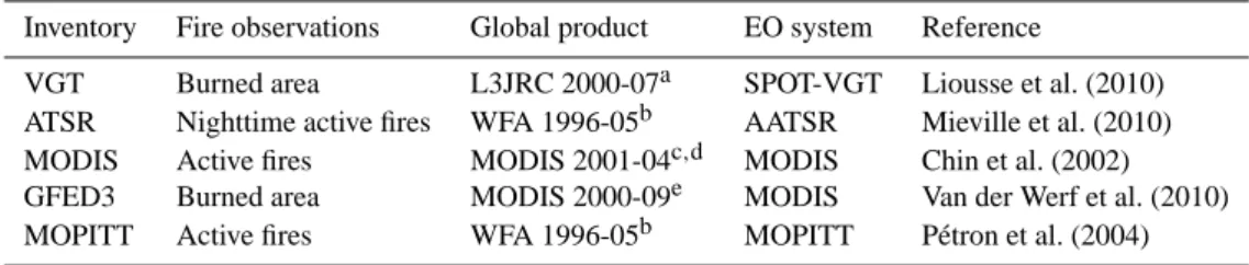
![Fig. 1. Maps of CO emissions [Tg] for the year 2003 for 0.5 ◦ grid cells; in the right lower corner the map of agreement (i.e](https://thumb-eu.123doks.com/thumbv2/123dok_br/16357652.190011/6.892.152.743.367.761/fig-maps-emissions-cells-right-lower-corner-agreement.webp)
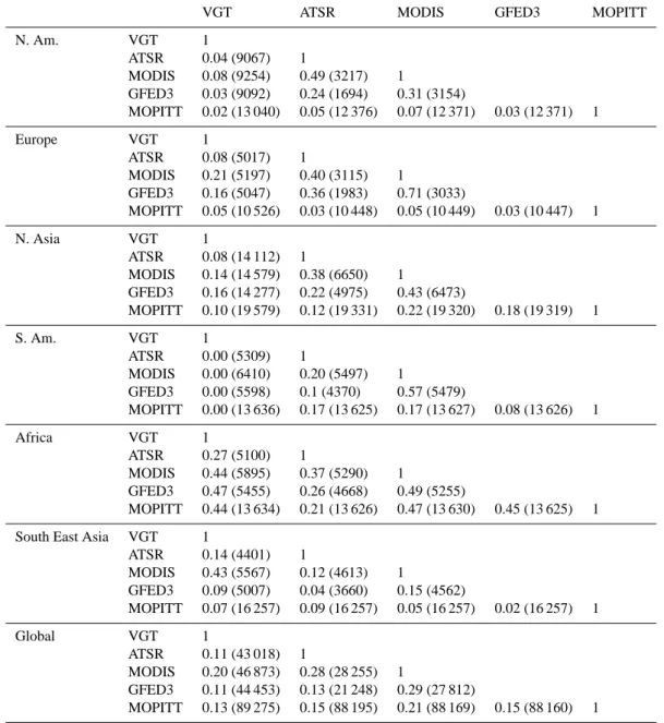
![Fig. 2. Seasonality of CO emissions [Tg CO month −1 ] for each continental window from the five inventories.](https://thumb-eu.123doks.com/thumbv2/123dok_br/16357652.190011/9.892.193.702.105.509/fig-seasonality-emissions-tg-month-continental-window-inventories.webp)
![Table 4. Spatial distribution [10 6 km 2 ] and proportion [%] of the area covered by each class for the continental windows and for the globe.](https://thumb-eu.123doks.com/thumbv2/123dok_br/16357652.190011/11.892.133.760.136.238/table-spatial-distribution-proportion-covered-class-continental-windows.webp)
![Fig. 3. Seasonality of CO emissions [Tg CO month −1 ] for the six continental windows and the three broad land cover types (forest, savanna/grassland and agriculture).](https://thumb-eu.123doks.com/thumbv2/123dok_br/16357652.190011/13.892.192.694.78.761/seasonality-emissions-continental-windows-forest-savanna-grassland-agriculture.webp)
